Multi-Scale Feature Mapping Network for Hyperspectral Image Super-Resolution

Abstract

Hyperspectral Image (HSI) can continuously cover tens or even hundreds of spectral segments for each spatial pixel. Limited by the cost and commercialization requirements of remote sensing satellites, HSIs often lose a lot of information due to insufficient image spatial resolution. For the high-dimensional nature of HSIs and the correlation between the spectra, the existing Super-Resolution (SR) methods for HSIs have the problems of excessive parameter amount and insufficient information complementarity between the spectra. This paper proposes a Multi-Scale Feature Mapping Network (MSFMNet) based on the cascaded residual learning to adaptively learn the prior information of HSIs. MSFMNet simplifies each part of the network into a few simple yet effective network modules. To learn the spatial-spectral characteristics among different spectral segments, a multi-scale feature generation and fusion Multi-Scale Feature Mapping Block (MSFMB) based on wavelet transform and spatial attention mechanism is designed in MSFMNet to learn the spectral features between different spectral segments. To effectively improve the multiplexing rate of multi-level spectral features, a Multi-Level Feature Fusion Block (MLFFB) is designed to fuse the multi-level spectral features. In the image reconstruction stage, an optimized sub-pixel convolution module is used for the up-sampling of different spectral segments. Through a large number of verifications on the three general hyperspectral datasets, the superiority of this method compared with the existing hyperspectral SR methods is proved. In subjective and objective experiments, its experimental performance is better than its competitors.

1. Introduction

The development of aerospace technology and remote sensing technology has promoted the application of hyperspectral image (HSI) based on remote sensing satellite [1,2,3,4], such as land monitoring [5,6], urban planning [7], road network layout [8], agricultural yield estimation [9] and disaster prevention and control [10]. However, due to the volume limitation of the imaging system and the need for system stability and time resolution, the acquisition of a large amount of spectral band information of hyperspectral images is often at the expense of spatial resolution [11]. Common methods to enhance spatial resolution are primarily studied from the aspects of hardware and process control. It not only challenges the current engineering technology but also violates the design concept of commercialization and miniaturization of remote sensing satellites.

In the field of image Super Resolution (SR), from the perspective of high-frequency detail similarity, researchers examine various ways to obtain more low-resolution image structure information and reconstruct high-quality HSI with detailed information. This technology is able to produce high-quality remote sensing images at a low cost without changing the existing hardware level. It has high research value and commercial prospects in the field of remote sensing data processing, and can immediately promote the development of commercial remote sensing satellites.

The concept of image super-resolution reconstruction originated from the research of Harris and Goodman [12,13] in 1964. The basic concept and method of image super-resolution were established by extrapolating the band limited signal. The early SR methods mainly include the interpolation-based method, reconstruction-based method and learning-based method.

Classical interpolation-based methods chiefly include zero-order interpolation (nearest neighbor interpolation), first-order interpolation (bilinear interpolation), and high-order interpolation (bicubic interpolation, cubic spline interpolation, and Lanczos interpolation), which will lead to blurred edges and artifacts. Considering the uneven distribution of image features, Duanmu et al. [14] and Zhang et al. [15], from the perspectives of Sobel operator and rational fractal interpolation, adopted distinct sampling methods for homogeneous regions and texture regions to overcome the blurring of edges. Furthermore, combined with a series of theories such as Discrete Wavelet Transform (DWT) [16], Whittaker filtering [17], partial Least squares method [18], Trilateral filter [19], high boost operator [20], etc., the interpolation method imbibed many aspects of optimization.

Given the defect that the interpolation algorithm cannot make full use of the abstract information of the image, starting from the Bayesian learning framework, the researchers prefer combining the process of the image degradation model with prior knowledge of the image to implement a reconstruction-based method [21,22,23,24].

Pickup et al. [25] marginalized potential parameters, such as geometric and photometric registration and image point spread function, to achieve a more realistic image prior distribution. To fuse high-resolution HSIs with low-resolution HSIs, Akhtar et al. [26] proposed a general Bayesian sparse coding strategy that merges combines Bayesian dictionaries for reconstructing the image. Based on the Bayesian framework, Zheng et al. [27] used a degenerate distribution method to derive an estimate of the analytical solution from enhancing the robustness of the algorithm. Irmak et al. [28] converted the ill-posed SR reconstruction problem in the spectral domain of HSIs into a secondary optimization problem in the abundance map domain based on the energy minimization method of the Markov random field.

Early learning-based methods are primarily to comprehend the mapping relationship between high-resolution images and low-resolution images. Drawing lessons from the sparse representation-based SR method proposed by Yang [29], Şimşek et al. [30] proposed an over-complete dictionary suitable for hyperspectral images to realize the learning of image mapping relations. Dong et al. [31] trained a variety of super-complete dictionaries based on different types of image blocks to effectively enhance the performance of the algorithm. Shao et al. [32] proposed a sparse autoencoder (CSAE) to effectively understand the mapping relationship between LR images and HR images.

In recent years, Convolutional Neural Network (CNN) has exhibited its powerful processing performance for various image tasks, such as image restoration [33], which continues the development of the natural image SR method based on the CNN network. Through supervised learning of the feature mapping relationship between the pairs of high-resolution (HR) images and low-resolution (LR) images, the SR method based on the CNN network can efficiently reconstruct high-quality images with rich details. Classical SR methods for natural images primarily include VDSR [34], EDSR [35], D-DBPN [36], and SAN [37]. The outstanding performance of these algorithms has inspired researchers to apply these methods to hyperspectral image reconstruction.

Due to the strong feature correlation between the adjacent bands of hyperspectral images, when CNNs are applied to the SR task of hyperspectral images, 3D convolution is required for feature extraction. Based on this, some classic algorithms have also been designed. For example, Mei et al. [38] used a 3D Fully Convolutional Network (3D-FCNN) to reconstruct images on a larger scale, thereby solving the problem of spectral information distortion while using traditional 2D convolution SR that is directly applied to hyperspectral images. Li et al. [39] used 2D units and 3D units to share spatial information in the image reconstruction process, which alleviated the problem of structural redundancy and led to a preliminary exploration of the lightweight hyperspectral models. Xie et al. [40] divided different spectral segments into multiple subsets, selected the key spectral segments of each subset for reconstruction, and guided the reconstruction of all spectral bands in the subsets, thereby achieving multiple reconstructions through asymptotic reconstruction. Different from the method of classifying and processing spatial and spectral information, Hu et al. [41] designed a spectral difference module, a parallel convolution module, and a fusion module for simultaneous super-resolution reconstruction of spatial and spectral information, which also enhances the generalization of the network. Li et al. [42] used MCNet based on the 2D/3D hybrid convolution module to further extract the potential features of the spectral image, but its complex 2D/3D conversion module still failed to mitigate the computational complexity.

At present, there are still many problems in the CNN-based SR method:

(1)

The parameters of the CNN model for hyperspectral images are still one or even several orders of magnitude higher than those of the CNN model for natural images at the same depth. Hence, the design of a network model with good performance with limited computing resources is the key to the practical application of the SR algorithm.

(2)

Most existing SR methods are learning for single-scale spectral features, which leads to the limited mining of spatial spectral information, making it impossible to reconstruct high-quality HR images for all the spectral segments.

(3)

Existing SR networks primarily focus on the impact of depth of the network on the overall performance and do not fully consider the further mining of the spectral feature information at each stage in the existing model.

Focusing on the problem of fully mining the prior knowledge of remote sensing images, and based on the SR method of classic CNN model, a variety of simple and effective CNN modules with different functions is designed from image feature extraction, feature nonlinear mapping, and image reconstruction.

Considering the above ideas, this paper proposes a Multi-Scale Feature Mapping Network (MSFMNet) for hyperspectral image super-resolution reconstruction. Using depthwise separable convolution, the multi-scale structure module based on wavelet transform and attention mechanism is designed, which can efficiently learn the prior knowledge of global and local features with a small number of model parameters. Therefore, the network model based on multi-scale structure can obtain more similar image feature information from low-resolution remote sensing image blocks. In each Multi-Scale Feature Mapping Block (MSFMB), the network can adaptively learn spectral features from each spatial scale and spectral band. Using four distinct evaluation indicators, the experimental results on three datasets demonstrate that the SR performance of the proposed MSFMNet for hyperspectral images is better than that of the existing hyperspectral SR methods. In this paper, the key contributions are as follows:

• The Multi-Scale Feature Mapping Block (MSFMB) is composed of up-sampling and down-sampling modules with depthwise separable convolution. After that, the spatial attention mechanism based on wavelet transform is integrated with the multi-scale module to generate features of different scales.
• In the nonlinear mapping stage of network features, a Multi-Level Feature Fusion Block (MLFFB) with few parameters is designed. After fusing the output features of each module, the self-attention mechanism based on pixel domain is used for linear weighting, and the feature information is used to assist the final image reconstruction.
• In the final stage of image reconstruction, the adaptive sub-pixel convolution is designed for the multi-channel characteristics of the hyperspectral image, addressing the problem that the effect of image reconstruction is limited by the limited-expression ability of nonlinear mapping in the reconstruction stage.
• A large number of experiments are carried out based on benchmark datasets, and the experimental results signify that the proposed method is superior to the existing methods.

2. Proposed Method

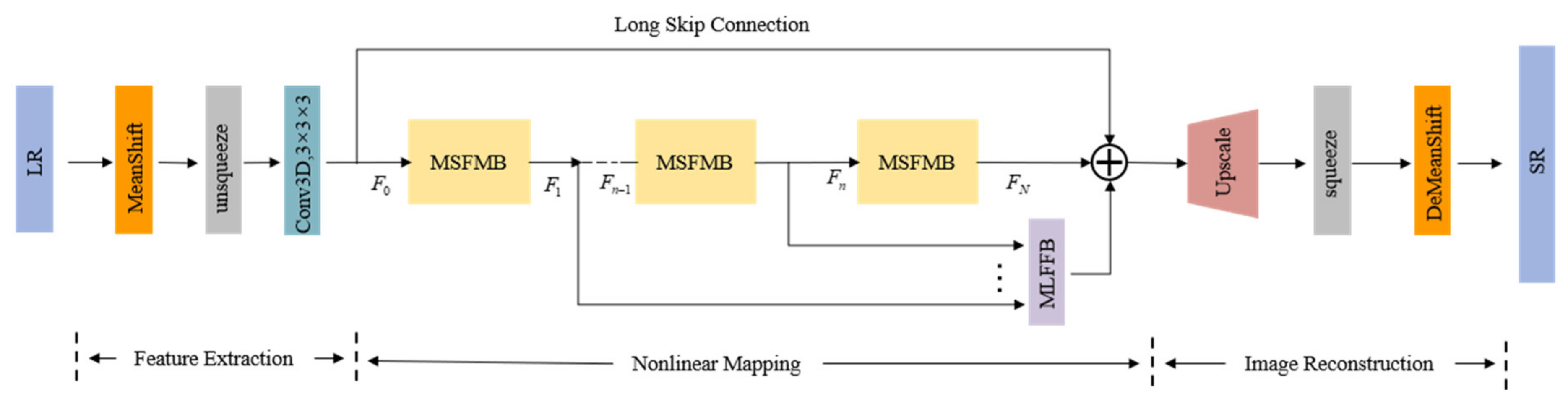
In this section, to better introduce the proposed work, the overall framework of MSFMNet is first briefed, which is shown in Figure 1. Different from the super-resolution task of ordinary images, hyperspectral remote sensing images have the characteristics of many spectral bands and large data amount of a single image. It is impossible to fully mine the spatial and spectral information of images only by using cascaded convolution to learn the features of local pixel regions. To solve the above problems, we designed several simple and effective networks in MSFMNET to extract and reconstruct spectral features from the two perspectives of feature nonlinear mapping and spectral segment reconstruction, which make the better reconstruction of spectral details of HSI. MSFMNet is chiefly composed of three parts: Feature Extraction Network ($H_{FE}$), Feature Nonlinear Mapping Network ($H_{MSFMB}$), and Image Reconstruction Network ($H_{UP}$).

Let $I_{LR}\in R^{H\times W\times B}$ denote the LR image and $I_{SR}\in R^{(\alpha H)\times (\alpha W)\times B}$ represent the reconstructed HR hyperspectral image, where $B$ is the number of spectral bands, $H$ and $W$, respectively, denote the length and the width of the image block, and $\alpha$ denotes the SR factor.

The $H_{FE}$ mainly uses the standardized operation to balance the distribution of the data. To preserve the geometric structure of the spectral image to the maximum extent, only 3D convolution is used to map the image features to a higher-dimensional feature space, and the initial feature $F_0\in R^{C\times B\times H\times W}$ is obtained. In the $H_{MSFMB}$, considering the up-sampling structure as the entry point, the cascaded MSFMB module is used to realize the residual feature extraction from various receptive fields.

The multi-level feature fusion network with a simple structure is simultaneously used for long-term and short-term memory to better improve the feature nonlinearity. Considering the characteristics of multi-spectral reconstruction in the $H_{UP}$, the sub-pixel convolution network is optimized based on the sub-pixel convolution design to better capture the information of spatial spectral characteristics and reconstruct the hyperspectral image by preserving rich details. More detailed information on each part is mentioned below.

2.1. Data Standardization

To reduce the difference between the data, the data demand standardization. Better data input can boost the convergence speed of the convolutional neural network and improve the image reconstruction effect of the overall network [43]. This method primarily uses zero-mean standardization (Z-score) for the data standardization process of the image feature extraction stage, which is a data standardization method that performs linear mapping on the basis of the mean and standard deviation of the data itself. First, stack the average values of the pixels of each band of the hyperspectral remote sensing image $I$ to obtain the mean vector, and then use the obtained mean vector $\mu$ to continue to solving the standard deviation vector $\sigma$ of each band.

During the network training, all input images are standardized, and the mathematical formula for specific implementation is specified in Equation (1):

$$x^{*}=\frac{x-\mu }{\sigma }$$

(1)

After zero-mean normalization, the data between different bands will be densely distributed around 0 mean, and the variance is 1.

After performing the image reconstruction, inverse normalization is performed according to the known standard deviation vector $\mu$ and mean vector $\sigma$, and a reconstructed high-resolution remote sensing image is obtained eventually.

2.2. Multi-Scale Residual Feature Network

To better protect the integrity of the spectral information and simplify the learning objectives and shortcomings of the spectral features, the network structure of RCAN [44] is used as a reference. The main body of the network adopts the jump connection method for residual learning, among which are several cascaded MSFMBs.

(1) Multi-scale Feature Fusion: The design of the MSFMB mainly draws on the theoretical and experimental derivations of CNF [45] and DBPN [36]. The size of the image features remains fixed in the depth direction of the overall network structure. Meanwhile, In MSFMB, up-sampling and down-sampling operations are carried out in the spatial domain with a scale factor of m, and three transformed features are fused to learn feature information of different scales, which can effectively prevent the loss of network performance caused by oversampling.

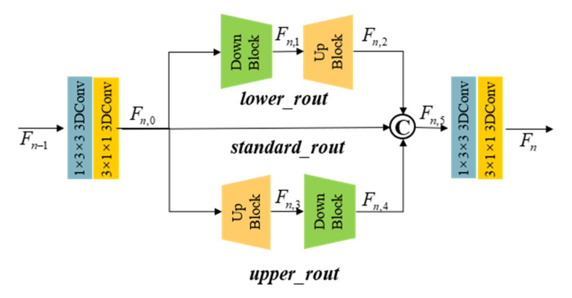
It can be observed from Figure 2 that when performing feature mapping in the MSFMB module, image features are primarily categorized into three paths, namely, lower_rout, standard_rout, and upper_rout. First, the input feature $F_{in}\in R^{C\times B\times H\times W}$ is subjected to the same-scale feature mapping through standard depthwise separable 3D convolution of standard_rout to obtain the F_std. In the upper_rout, the F_std is passed through the up-sampling module to obtain the feature $F_{up}^0\in R^{C\times B\times mH\times mW}$, and then the down-sampling module is used to bring it back to the original size, that is, feature $F_{up}\in R^{C\times B\times H\times W}$. Similarly, in the lower_rout, F_std is passed through the down-sampling module to obtain the feature $F_{down}^0\in R^{C\times B\times (H/m)\times (W/m)}$, and it is restored to its original size through the up-sampling module to obtain $F_{down}\in R^{C\times B\times H\times W}$. Eventually, after concatenating the F_std, F_up, and F_down and using the standard depthwise separable 3D convolution to achieve feature fusion and channel reduction, the output feature $F_{out}\in R^{C\times B\times H\times W}$ with the channel C is derived. The mathematical representation of the MSFMB module is mentioned below.

$$F_{std}=f[w_p\ast f(w_d\ast F_{in})]$$

(2)

$$F_{up}=g^{\downarrow }[g^{\uparrow }(F_{std})]$$

(3)

$$F_{down}=g^{\uparrow }[g^{\downarrow }(F_{std})]$$

(4)

$$F_{out}=f\{w_p\ast f[w_d\ast C(F_{std},F_{up},F_{down})]\}$$

(5)

where $w_d$ represents the convolution kernel of depthwise convolution with a size of 3 × 3 × 3, group is set to C, $w_p$ denotes the convolution kernel of a pointwise convolution with a size of 1 × 1 × 1, $f$ indicates the LeakyReLU activation function, * represents the convolution, $C(\cdot )$ stands for the concatenation operation, and $g^{\downarrow }$ and $g^{\uparrow }$ denote the up-sampling module and the down-sampling module.

Compared to multi-level up-sampling and down-sampling structure in LapSRN [46] and the alternate up-sampling and down-sampling feature extraction structure in DBPN [36], this module not only focuses on large-scale or small-scale feature information in the depth direction, but also considers the characteristics of three kinds of feature information to greatly enrich the prior knowledge that can be obtained by feature extraction. Meanwhile, since only the single-stage up-sampling and down-sampling is performed, information loss caused by excessive noise introduced during the sampling process can be substantially avoided.

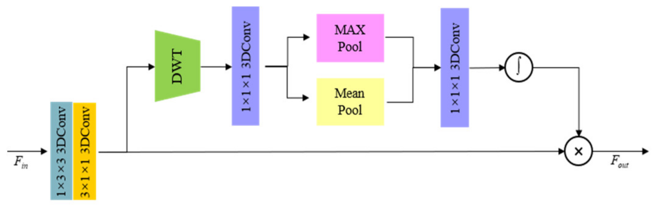
(2) Feature multi-scale transformation: The structure based on the self-attention mechanism is widely used in natural image SR methods. For the complex characteristics of spectral features, when performing multi-scale feature nonlinear mapping, a novel spatial attention structure based on DWT is proposed for detailed feature extraction.

The design of the wavelet-based spatial attention mechanism is highlighted in Figure 3. First, for the spectral feature $F_{in}\in R^{C\times B\times H\times W}$, the scale transformation with a sampling factor of m is performed through the depthwise separable convolution to obtain $F\in R^{C\times B\times mH\times mW}$, and then the four-layer image feature comprising $F_{LL}$, $F_{LH}$, $F_{HL}$, and $F_{HH}$ is obtained after the DWT is performed. Since the low-frequency information $F_{LL}$ contains less detailed information, only $F_{LH}$, $F_{HL}$, and $F_{HH}$ are used for feature guidance when performing feature fusion. Since the spatial scales of the features obtained by DWT and the original features may be different, it is mandatory to use interpolation to restore to the original size, and use standard 3D convolution for feature dimension fusion. The standard 3D convolution kernel is 1 × 1 × 1, and the output features are determined as $F_{Fusion}$. After that, Global Max Pooling and Global Average Pooling are performed to obtain the two single-layer feature $F_{avg}^w\in R^{1\times B\times H\times W}$ and $F_{\max }^w\in R^{1\times B\times H\times W}$, and the standard convolution is used for fusion to generate two-dimensional features. After Sigmoid activation function, the weight coefficient $M_w\in R^{1\times B\times H\times W}$ is obtained, which is applied to $F$ for feature optimization. The mathematical expression of the spatial attention sampling module based on DWT can be expressed by the following formula:

$$F=f[w_p\ast f(w_d\ast F_{in})]$$

(6)

$$F_{LL},F_{LH},F_{HL},F_{HH}=DWT(F)$$

(7)

$$F_{Fusion}=w_{3d1}\ast I[C(F_{LH},F_{HL},F_{HH})]$$

(8)

$$\begin{array}{l}{M}_w(F)=\sigma [w_{3d1}\ast C(F_{avg}^w,F_{\max }^w)]\otimes F\\ =\sigma \{w_{3d1}\ast C[AvgPool(F_{Fusion}),Maxpool(F_{Fusion})]\}\otimes F\end{array}$$

(9)

where $DWT(\cdot )$ denotes the discrete wavelet transform, $w_{3d1}$ stands for standard 3D convolution with a convolution kernel size of 1 × 1 × 1, I represents the sampling to a sampling operation consistent with the spatial size of the feature F, $\sigma$ denotes the sigmoid activation function, and $\otimes$ represents the matrix point multiplication. For the down-sampling module, $w_d$ represents a depthwise convolution with a size of 3 × 3 × 3, Group is set to C, and stride is set as 2. For the up-sampling module, $w_d$ represents a depthwise transposed convolution with a size of 3 × 3 × 3, Group is set to C, and stride is set as 2.

2.3. Multi-Level Feature Fusion Block

In the earlier densely connected structures, such as DenseNet [47] and SRDenseNet [48], the output results of each level of convolution or modules are directly added or concatenated as the input of the next level. 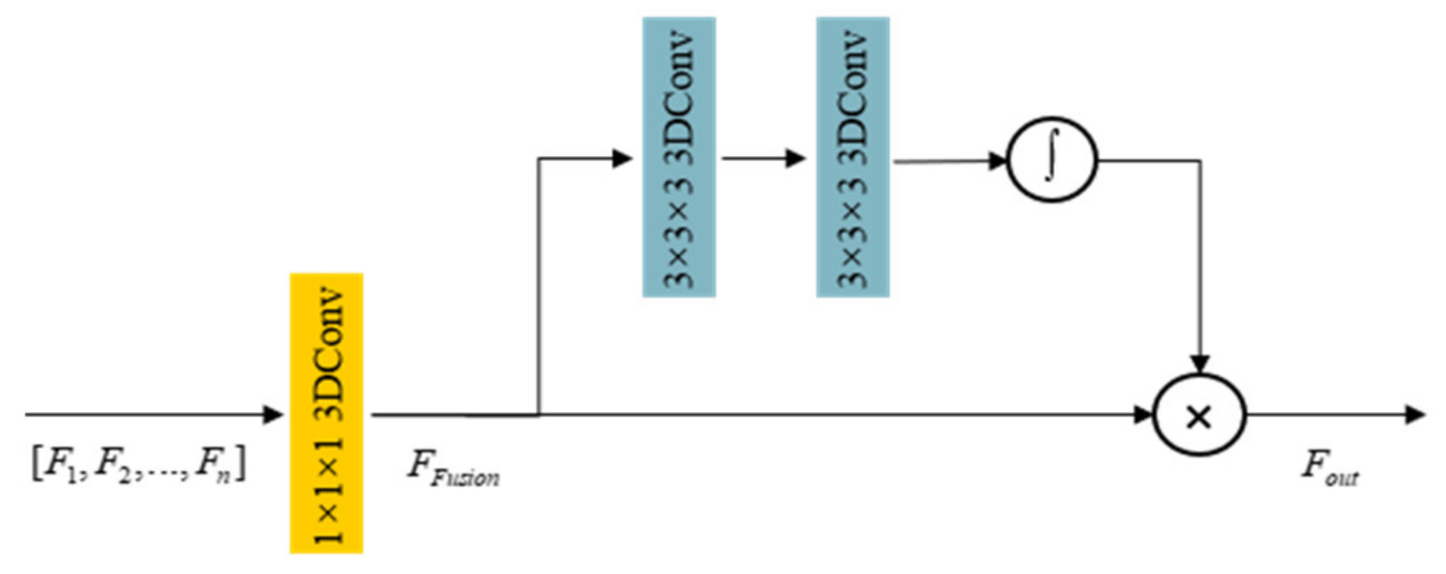In order to better integrate the output results of all levels of modules to assist in the reconstruction of the final features, when the bypass connection is established, inspired by PAN [49], we propose the Multi-Level Feature Fusion Block (MLFFB) based on the spatial attention mechanism, which can generate more detailed features. The network structure of the MLFFB is illustrated in Figure 4.

Assuming that there are a total of n MSFMB in the feature nonlinear mapping stage of the network, in the MLFFB, first take the output $F_i\in R^{C_{in}\times B\times H\times W}$ of the first n − 1 modules for stacking, where $i\in [1,\dots ,n-1]$. The convolution kernel $w_{3d1}$ with a size of 1 × 1 × 1 performs the dimensionality reduction processing of the channel dimension to obtain $F_{fusion}\in R^{C_{in}\times B\times H\times W}$. Then, according to the channel down-sampling factor q, the convolution kernel $w_{3d1}$ with kernel dimension of 1 × 1 × 1 performs channel-dimensional down-sampling to obtain $F_{down}\in R^{(C_{in}/q)\times B\times H\times W}$. After that, we use the convolution kernel $w_{3d1}^{\uparrow }$ and the kernel of 1 × 1 × 1 to perform the channel-dimensional up-sampling to obtain $F_{up}\in R^{C_{in}\times B\times H\times W}$. Finally, a sigmoid activation function is used to normalize $F_{up}$ and generate attention weight coefficients, which can apply to linearly weight the $F_{fusion}$ features to obtain the auxiliary feature $F_{out}$:

$$F_{fusion}=w_{3d1}^{\downarrow }\ast C(I_1,I_2,\dots ,I_{n-1})$$

(10)

$$F_{out}=F_{fusion}\ast \sigma [w_{{}_{3d1}}^{\uparrow }\ast (w_{{}_{3d1}}^{\downarrow }\ast F_{fusion})]$$

(11)

The multi-level feature extraction module optimizes and improves the information reuse rate of the feature maps at each level by introducing a self-attention mechanism based on the pixel domain, and significantly improves the performance of feature mapping in the nonlinear mapping stage.

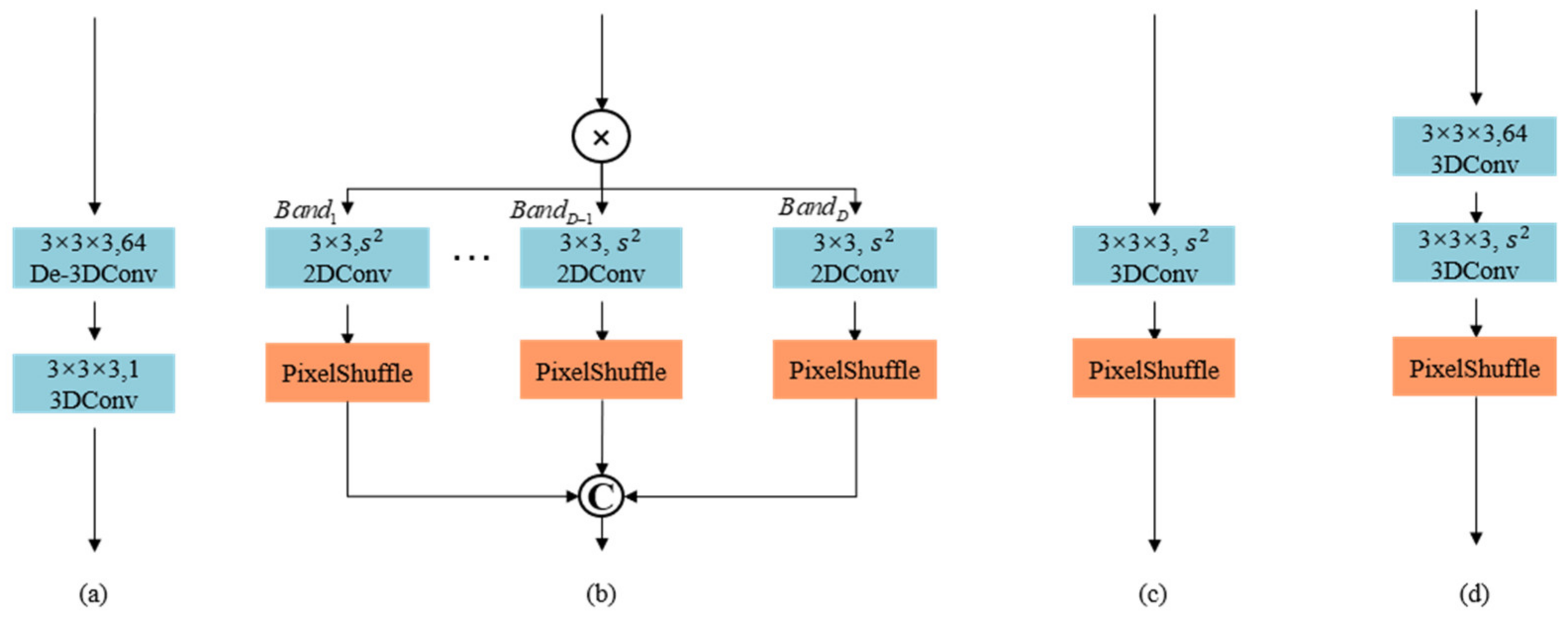
2.4. Image Reconstruction

Common image reconstruction modules in the SR method include deconvolution [50] and 2D sub-pixel convolution [51]. Aiming at the problem of multi-band feature reconstruction of remote sensing hyperspectral images, we optimize the sub-pixel convolution, and propose a 3D-based sub-pixel convolution method for the image reconstruction network of MSFMNet. The structure is shown in Figure 5d. Through experiments, we have proved that its effect is better than other structures of Figure 5.

The 3D-based sub-pixel convolution is primarily divided into three parts: feature fusion, channel compression and pixel rearrangement. The input feature $F_{Fusion}$ in the feature reconstruction stage is obtained by summing the output $F_{Fea}$ of the feature extraction stage, the fusion feature $F_{Assist}$ of the auxiliary module, and the output $F_{map}$ of the network nonlinear mapping stage. To ensure the reconstruction effect after channel compression, further fusion for $F_{Fusion}$ is required through 3D convolution, whose kernel is $w_{3d3}^{’}$ and its size is 3 × 3 × 3.

Before the pixelshuffle operation, channel compression of features is performed by using a 3D convolution kernel $w_{3d3}^{’}$, where the size of whom is 3 × 3 × 3 and the output channel is the square of the reconstruction factor $s$. Eventually, the pixelshuffle operation $h_{ps}^{\uparrow }(\cdot )$ and the inverse normalization is used to achieve reconstruction of the SR spectral image. The specific formula is as follows:

$$F_{sr}=h_{ps}^{\uparrow }\{w_{3d3}^{’’}\ast [w_{3d3}^{’}\ast (F_{Fea}+F_{Assist}+F_{map})]\}$$

(12)

$$I_{sr}=F_{sr}\ast \sigma +\mu$$

(13)

The L1 norm is applied to the network as a loss function for network training, and its mathematical expression is mentioned in the following formula:

$$L_{MAE}\left(I_{hr},I_{sr}\right)=\frac{1}{N}{\displaystyle \sum _{i=1}^N\left|I_{hr}^i-I_{sr}^i\right|}$$

(14)

where $I_{SR}$ represents the reconstructed spectral image, $I_{hr}$ is the original spectral image, and N stands for the number of training samples.

3. Experiments

To verify the performance of the proposed MSFMNet, in this section, we first introduce three common datasets. Then, the specific implementation details and evaluation indexes is mentioned. Finally, we compare the performance of MSFMNet with the existing algorithms.

3.1. Experimental Settings

(1) Datasets: Three widely used HSI datasets are used here to evaluate the model performance of the MSFMNet method. When generating the training set, $I_{sr}$ is generated based on the requirements of specific up-sampling factor, and the $I_{hr}$ and $I_{sr}$ are cropped according to the fixed stride and side length.

CAVE: The CAVE dataset is a 400 nm–700 nm hyperspectral dataset collected by a Cooled CCD camera. A total of 31 bands are collected at an interval of 10 nm each. The dataset contains 32 hyperspectral images with a size of 512 × 512 × 31. For HSIs, 7 images are selected as the test set and the remaining 25 as the training set.

Pavia Center and Pavia University: The Pavia Center dataset (Pavia) and the Pavia University (PaviaU) dataset are collected by ROSIS sensors over the city of Pavia in northern Italy, with a wavelength range of 430 nm–860 nm. Among them, the size of the Pavia dataset is 715 × 1096 × 102, and the size of the PaviaU dataset is 610 × 340 × 103. For the two datasets, the 144 × 144 spectral image with the upper left corner as the origin is used as the test set, and the other parts are used as the training set.

The main difference: the number of bands in the CAVE dataset is significantly smaller than that of Pavia and PaviaU, but the number of scenes is much larger than that of Pavia and PaviaU. The number of bands of Pavia and PaviaU is similar, but the picture size is very different. Compared with a single spectrum, the size of Pavia is almost four times that of PaviaU, so in the training phase, PaviaU has the fastest training speed.

(2) Implementation Details: According to different hyperspectral datasets, the spectral bands B of the model is set as the spectral bands of datasets. In the MSFMNet, the DWT uses Gabor wavelet for multi-direction feature extraction, and the number of feature layers is set to 64, that is, the channel C is 64. In the feature nonlinear mapping network, in order to better achieve feature extraction, a total of four MSFMB are used in series, so a total of three groups of features are cascaded as the input of MLFFB. In MLFFB, the down-sampling factor q in the pixel domain attention mechanism is set to 8. In MSFMB, both the up-sampling and down-sampling factors of the feature are set to 2.

All the experiments and test processes are run in MATLAB and Pytorch environments, and the hardware configuration is four NVIDIA RTX2080Ti graphics cards with 11 GB of memory.

When setting the training-related hyperparameters, the Adam method is selected as the network optimization method to optimize and update the parameters. The algorithm in this paper sets the exponential decay rate of Adam’s biased first-order moment estimation and biased second-order moment estimation to 0.9 and 0.999, respectively. The value of the correction factor is set to ${10}^8$, and the step size is set to 0.001. In network training, the initial learning rate is set to ${10}^4$, the attenuation coefficient is 0.1 for every 120 rounds, and a total of 400 rounds are trained. At the beginning of network training, Pyotrch’s weight_norm function is used to initialize the weights. To maintain the spatial size of the feature after convolution, zero padding is used in all the convolution layers.

(3) Evaluation Metrics: The performance differences of different methods are primarily evaluated from subjective and objective indicators. In order to be more in line with the subjective perception of the human eye, RGB images and error images are provided for visual comparison.

To qualitatively measure the proposed MSFMNet, four evaluation methods are employed to verify the effectiveness of the algorithm, including Peak Signal-to-Noise Ratio (PSNR), Mean Peak Signal-to-Noise Ratio (MPSNR), Structural Similarity (SSIM), and Spectral Angle Mapping (SAM). They are defined as:

$$MSE=\frac{1}{M\times N}{\displaystyle \sum _{i=1}^M{\displaystyle \sum _{j=1}^N{[X(i,j)-Y(i,j)]}^2}}$$

(15)

$$PSNR=10\times {\log }_{10}\left({[2^{Bits}-1]}^2/MSE\right)$$

(16)

$$MPSNR=\frac{10}{B}{\displaystyle \sum _{i=1}^B{\log }_{10}\frac{{\left(2^{Bits}-1\right)}^{2}MN}{{\displaystyle \sum _{i=1}^M{{\displaystyle \sum _{j=1}^N\left(X\left(i,j\right)-Y\left(i,j\right)\right)}}^2}}}$$

(17)

where X and Y denote the reconstructed image $I_{sr}$ and the original image $I_{hr}$, M and N stand for the image length and width, respectively, the MSE represents mean square error, Bits denotes the image pixel depth, and B stands for HSI spectral bands.

$$SSIM=\frac{\left(2{\mu }_x{\mu }_y+C_1\right)\left(2{\sigma }_x{}_y+C_2\right)}{\left({\mu }_x{}^2+{\mu }_y{}^2+C_1\right)\left({\sigma }_x{}^2+{\sigma }_y{}^2+C_2\right)}$$

(18)

where ${\mu }_x$ and ${\mu }_y$ represent the mean of $I_{sr}$ and $I_{hr}$, ${\sigma }_x$ and ${\sigma }_y$ denote the variance of $I_{sr}$ and $I_{hr}$, and C₁ and C₂ are both minimum that prevent division by zero.

$$\theta ({\mathrm{z}}^{*},{\mathrm{z}}_h)={\cos }^{-1}(\frac{z_h^T{z}^{*}}{(‖{\mathrm{z}}_h‖)(‖{\mathrm{z}}^{*}‖)})={\cos }^{-1}(\frac{z_h^T{z}^{*}}{\sqrt{{(z^{*})}^T{z}^{*}}\sqrt{{\mathrm{z}}_h^T{\mathrm{z}}_h}})$$

(19)

$$SAM=\frac{1}{HW}{\displaystyle \sum _{i=0}^H{\displaystyle \sum _{j=0}^W\theta (X(i,j),Y(i,j))}}$$

(20)

where ${\mathrm{z}}^{*}$ represents the pixel vector of $I_{sr}$, ${\mathrm{z}}_h$ represents the pixel vector of $I_{hr}$, and $\theta$ stands for the spectral angle mapping of a single pixel vector.

3.2. Results and Analysis

To evaluate the performance of the MSFMNet method as comprehensively as possible, several popular SR methods are used for comparison, including four commonly used algorithms, namely Bicubic, VDSR, EDSR, ERCSR, and MCNet. The subjective and objective test results of the three HSI datasets are mentioned below.

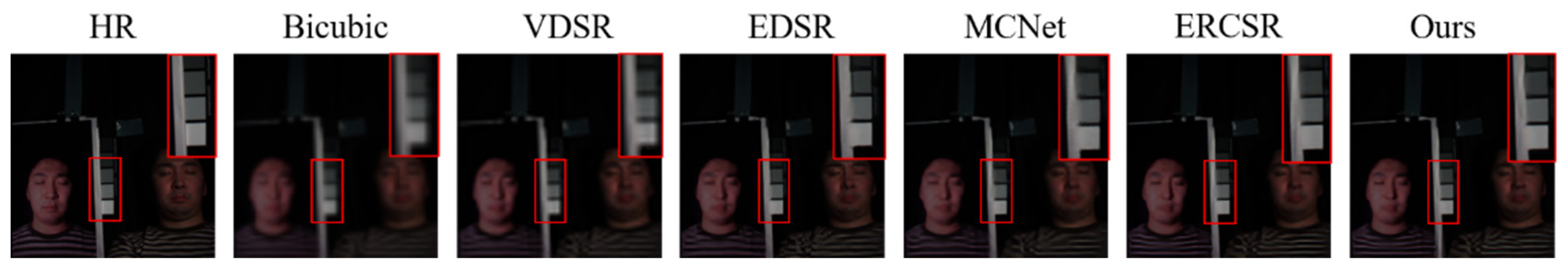
(1) CAVE Dataset: In Figure 6, the 26th, 17th, and 9th bands are served as the R-G-B channels to visualize the test RGB images of the photo_and_face_ms in the CAVE dataset that are generated by different methods with a scale factor of 8. It can be obviously observed that the details of the hyperspectral reconstructed images obtained by Bicubic, VDSR, EDSR, MCNet, and ERCSR are quite different from the original images, especially those obtained by Bicubic and VDSR. In addition, due to the lack of learning between spectral features, the face part of the image generated by EDSR is very blurry. Although MCNet and ERCSR utilizes spectral features based on 2D/3D convolution, there is still a slight spatial distortion in the bright region. From the perspective of visual effects, MSFMNet is superior to other methods. 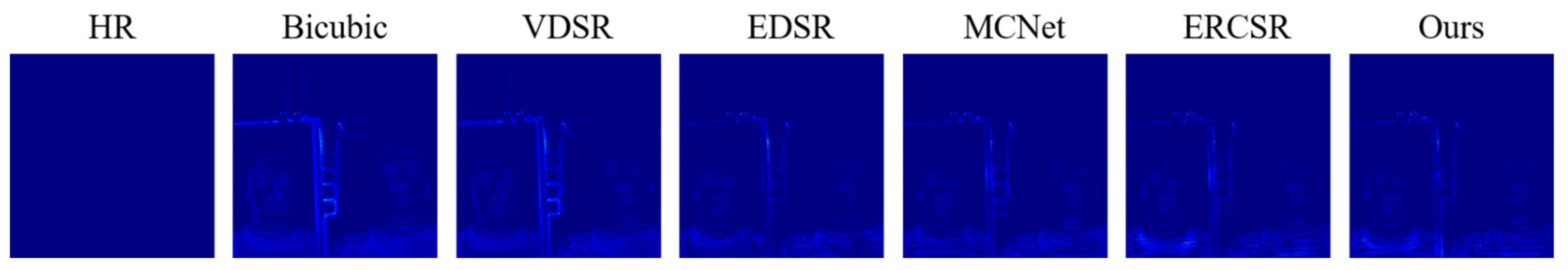Figure 7 displays the pixel absolute difference images between the image reconstructed by various methods and the original image. For MLFFB is used for multi-level feature fusion, the reconstruction effect of MSFMNet on the edge of the photo frame and the face part is much closer to the original image.

To further demonstrate our superiority in the reconstruction of spectral information, the reflectivity of pixels in the photo_and_face_ms image in different spectral bands is randomly selected in Figure 8. It is obvious that the spectral information generated by MSFMNet is closest to the HR image. The first few bands contain less bright information, and it is difficult to reflect the difference in algorithm performance. As the spectral wavelength increases, the detailed information of the band gradually accumulates, and the difference in the detail reconstruction ability of different algorithms becomes prominent. At the same time, due to the use of data standardization, the proposed method is also sensitive to the small number of features in the first few bands, which also helps to reconstruct the overall details of HSI.

For quantitative evaluation in a wider range of scenarios and indicators,

Table 1. Quantitative evaluation on the cave dataset of state-of-the-art hyperspectral image sr algorithms: average psnr/mpsnr/ssim/sam for scale factors 2, 4, and 8.

Scale	Methods	PSNR ↑	MPSNR ↑	SSIM ↑	SAM ↓
	Bicubic	40.330	39.500	0.9820	3.311
	VDSR	44.456	43.531	0.9895	2.866
×2	EDSR	45.151	44.207	0.9907	2.606
	MCNet	45.878	44.913	0.9913	2.588
	ERCSR	45.972	45.038	0.9914	2.544
	MSFMNet	46.015	45.039	0.9917	2.497
	Bicubic	34.616	33.657	0.9388	4.784
	VDSR	37.027	36.045	0.9591	4.297
×4	EDSR	38.117	37.137	0.9626	4.132
	MCNet	38.589	37.679	0.9690	3.682
	ERCSR	38.626	37.738	0.9695	3.643
	MSFMNet	38.733	37.814	0.9697	3.676
	Bicubic	30.554	29.484	0.8657	6.431
	VDSR	32.184	31.210	0.8852	5.747
×8	EDSR	33.416	32.337	0.9002	5.409
	MCNet	33.607	32.520	0.9125	5.172
	ERCSR	33.624	32.556	0.9113	5.116
	MSFMNet	33.675	32.599	0.9136	5.084

Bold values represent the best result and underlined values represent the second best.

lists the results of four performance indicators in CAVE datasets with scale factors of 2, 4, and 8, with the optimal results represented in bold font. It is clear from the quantitative results of the four indicators that MSFMNet has achieved the best results of all the methods. Due to the use of depthwise separable 3D convolution and multi-scale feature mapping, our method realizes the fusion of feature information of different spatial sizes while mining the relevant information between spectral segments. In this way, MSFMNET can estimate the height of HSIs containing a lot of spatial spectral information.

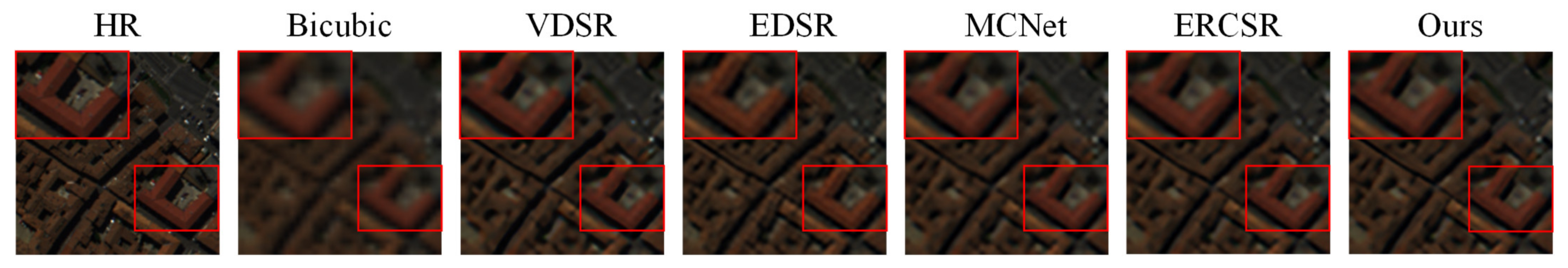
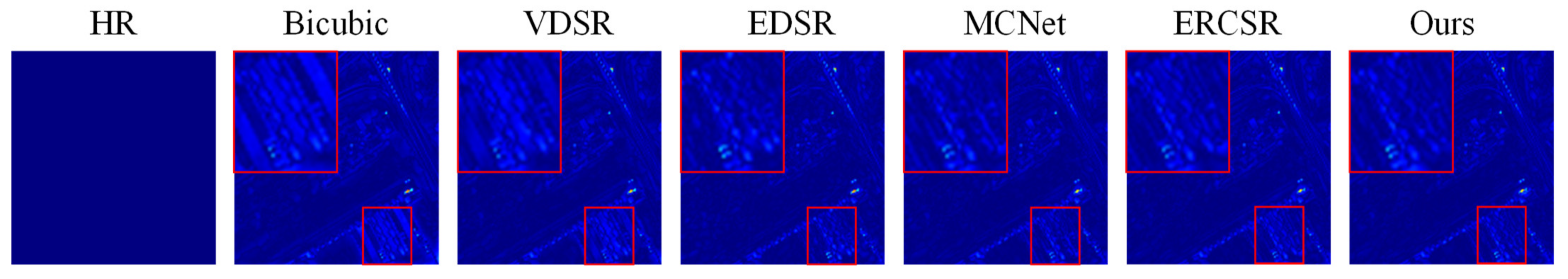
(2) Pavia Dataset: Figure 8 shows the comparison of reconstruction effects of different methods in the Pavia dataset when the scale factor is 4. Among them, the 13th, 35th, and 60th bands are used for color image generation. It can be seen that the Bicubic, EDSR, MCNet, and ERCSR estimates are fuzzy and lack enough details, while the VDSR overfits, resulting in too sharp texture. Only MSFMNet can reconstruct the real details without distortion.

As the error images in Figure 9 shows, for a complex environment with a large number of details, Bicubic could not recover details well, while VDSR, EDSR, ERCSR, and MCNet and ERCSR could only recover details of the part street. The difference between the street details generated by the MSFMNet and the original image was smaller. This proves that MSFMNet has a very good performance in the reconstruction of complex structural information. In terms of spectrum, we select pixels randomly from the image, and plot the reflectance of different bands in Figure 9. It is obvious that the reflectance of the proposed method is the closest to the original image, which demonstrates the superiority of the MSFMNet method in spectrum generation. Due to the normalization of the input and the use of 3D sub-pixel convolution for image reconstruction, our method is more stable in terms of spatial spectral consistency.

Table 2. Quantitative evaluation on the Pavia dataset of state-of-the-art hyperspectral image sr algorithms: average psnr/mpsnr/ssim/sam for scale factors 2, 4, and 8.

Scale	Methods	PSNR ↑	MPSNR ↑	SSIM ↑	SAM ↓
	Bicubic	32.406	31.798	0.9036	4.370
	VDSR	35.392	34.879	0.9501	3.689
×2	EDSR	35.160	34.580	0.9452	3.898
	MCNet	35.124	34.626	0.9455	3.865
	ERCSR	35.602	35.099	0.9506	3.683
	MSFMNet	35.678	35.200	0.9506	3.656
	Bicubic	26.596	26.556	0.7091	7.553
	VDSR	28.328	28.317	0.7707	6.514
×4	EDSR	28.649	28.591	0.7782	6.573
	MCNet	28.791	28.756	0.7826	6.385
	ERCSR	28.862	28.815	0.7818	6.125
	MSFMNet	28.920	28.873	0.7863	6.300
	Bicubic	24.464	24.745	0.4899	7.648
	VDSR	24.526	24.804	0.4944	7.588
×8	EDSR	24.854	25.067	0.5282	7.507
	MCNet	24.877	25.096	0.5391	7.429
	ERCSR	24.965	25.190	0.5382	7.834
	MSFMNet	25.027	25.257	0.5464	7.449

Bold values represent the best result and underlined values represent the second best.

lists the quantitative performance of all methods on the test set with scale factors of 2, 4, and 8. The results show that the performance of the proposed method is superior to other algorithms on three scales. Meanwhile, different from CAVE dataset, because the dataset of Pavia scene is small, this experiment also proves that MSFMNet has a better processing effect on a small dataset.

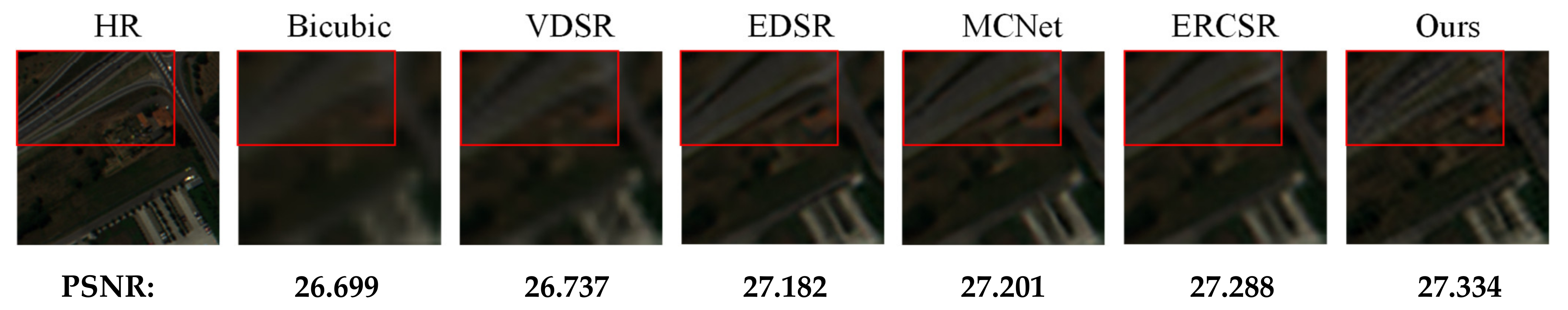
(3) PaviaU Dataset: Figure 10 shows the RGB images of all the methods with a scale factor of 8. It can be seen from the figure that most of the methods, such as Bicubic, EDSR, and VDSR cannot reconstruct the road details very well. The road details generated by MCNet and ERCSR are relatively vague, and some road details are missing, so it is impossible to reconstruct the real road details. MSFMNet can effectively carry out detailed reconstruction of the road. 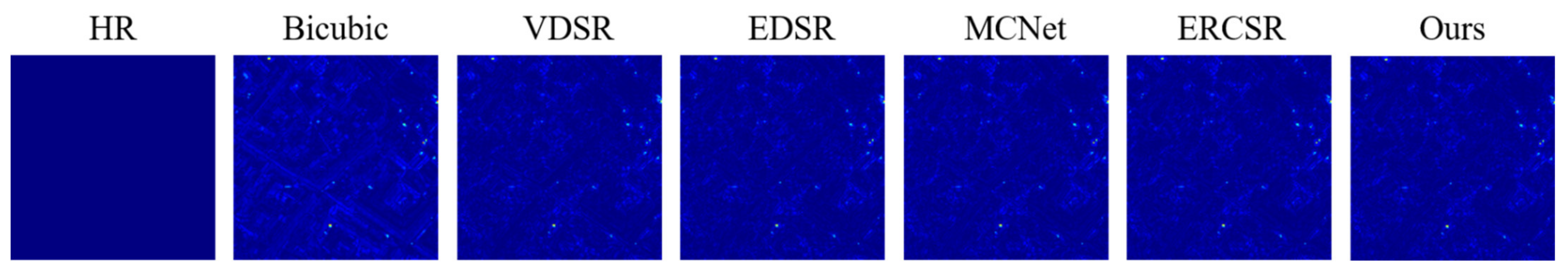Figure 11 shows the error images of different methods on the PaviaU dataset. Obviously, the error of HSIs reconstructed by the proposed method is the smallest.

Table 3. Quantitative evaluation on the PaviaU dataset of state-of-the-art hyperspectral image sr algorithms: average psnr/mpsnr/ssim/sam for scale factors 2, 4, and 8.

Scale	Methods	PSNR ↑	MPSNR ↑	SSIM ↑	SAM ↓
	Bicubic	30.509	30.497	0.9055	3.816
	VDSR	33.988	34.038	0.9524	3.258
×2	EDSR	33.943	33.985	0.9511	3.334
	MCNet	33.695	33.743	0.9502	3.359
	ERCSR	33.857	33.910	0.9520	3.220
	MSFMNet	34.807	34.980	0.9582	3.160
	Bicubic	29.061	29.197	0.7322	5.248
	VDSR	29.761	29.904	0.7854	4.997
×4	EDSR	29.795	29.894	0.7791	5.074
	MCNet	29.889	29.993	0.7835	4.917
	ERCSR	30.049	30.164	0.7899	4.865
	MSFMNet	30.140	30.283	0.7948	4.861
	Bicubic	26.699	26.990	0.5936	7.179
	VDSR	26.737	27.028	0.5962	7.133
×8	EDSR	27.182	27.467	0.6302	6.678
	MCNet	27.201	27.483	0.6254	6.683
	ERCSR	27.288	27.548	0.6276	6.611
	MSFMNet	27.334	27.586	0.6356	6.615

Bold values represent the best result and underlined values represent the second best.

displays the quantitative analysis results. From the perspective of reconstruction of spatial information and reduction of distortion of spectral information, MSFMNet is obviously superior to other methods. In conclusion, it can be seen from the experimental results and analysis that the MSFMNet method shows superior performance in HSI SR tasks. In the next section, further analysis is given to verify that the performance in each part of the model is from multiple aspects.

3.3. Ablation Study

(1) Component Analysis: In this section, we analyze whether sufficient experiments are conducted, including a study of the MSFMB module and ablation study analysis. To make a simple and fair comparison, we analyze the results for a scale factor of 2 are analyzed on the PaviaU dataset.

Table 4. Ablation study results on evaluating the efficiency of the network structure.

	1	2	3	4	5	6	7
MSFMB	√	√	√	√	√	√	√
SA	×	√	√	√	√	√	√
DWT	×	×	√	√	√	√	√
MLFFB	×	×	×	√	×	×	√
PixelShuffle	×	×	×	×	√	×	√
MeanShift	×	×	×	×	×	√	√
PSNR	34.113	34.151	34.215	34.558	34.461	34.525	34.807

reflects the impact of ablation research on the multi-scale module, attention mechanism, wavelet transform, multi-level feature extraction module, adaptive sub-pixel convolution, and MeanShift. Different component combinations are set to analyze the performance of the proposed MSFMNet. To make a fair comparison, a network with seven modules has been chosen here to conduct the ablation surveys.

First, when the network does not contain multi-scale modules, multi-level feature extraction modules, and adaptive sub-pixel convolution, MeanShift, which only contains 3D units produces the worst performance. It chiefly lacks sufficient learning of effective features, which also signifies that spectral and spatial features cannot be extracted properly without these components. Therefore, these components are mandatory for the suggested network. Then, MSFMB is added to the baseline. Moreover, the PSNR showed that the model performance was improved. Then, two of these components are added to the baseline. Compared to the previous evaluations, the evaluation indicators have produced relatively better results. In short, experiments prove that each component can significantly enhance the performance of the network. This suggests that each component plays a key role in making the network easier to train. Finally, the other three components are individually attached to the baseline. The table highlights that the results of the three components are significantly better than the performance of only one component, which demonstrates the effectiveness and benefits of the suggested components.

(2) Image reconstruction network: In this section, the PaviaU dataset has been used to perform reconstruction with a scale factor of 2 and compare the four reconstruction structures. The specific objective index results are enlisted in

Table 5. Comparison of different reconstruction modules under the same network structure in the Pavia dataset with a scale factor of 2.

	3D Conv	2D Sub-Pixel	3D Sub-Pixel	Optimized 3D Sub-Pixel
PSNR	35.641	35.545	35.648	35.678
MPSNR	35.171	35.077	35.153	35.200
SSIM	0.9502	0.9495	0.9502	0.9506
SAM	3.703	3.718	3.710	3.656
Parm (×105)	1.9	1.8	0.069	1.1

. It can be observed from the comparison results that the reconstruction performance of different reconstruction modules is quite different. Compared to the original 2D sub-pixel convolution, the improved 3D sub-pixel convolution improves the PSNR index by almost 0.13 dB. Meanwhile, Table 5 validates the overall parameters of the four types of structures. From the comparison, it can be noticed that the parameter is not the only factor that determines the performance of the image reconstruction. The Optimized 3D sub-pixel convolution effectively reconstructs the detailed information of HSI.

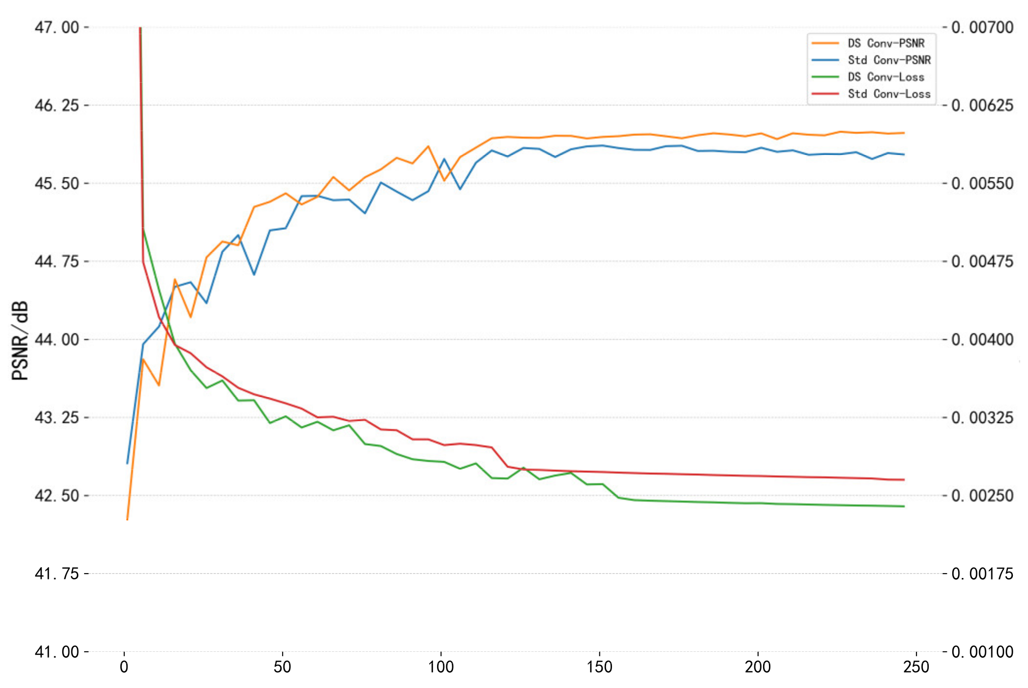
(3) The influence of the type of convolution: To choose a better convolution method, the similarities and differences between the depthwise separable convolution and the standard 3D convolution, the amount of convolution kernel parameters, and the network training duration will be compared in detail. This experiment focuses on the actual performance of the two types of convolution in the network and explores the basic convolution unit suitable for this algorithm. In this experiment, the CAVE dataset was used as the experimental dataset and the comparison of two-fold super-resolution reconstruction was executed.

Figure 12 is a line chart showing explaining the convergence process of different convolutions based on the MSFMNet network structure. From the line chart of performance comparison, it can be seen noticed that due to the small parameter amount of the depthwise separable convolution, it has the characteristics of greater depth, based on the depth separability. The convergence effect of the convolutional network model is always better than that of the standard convolutional network model.

Table 6. Comparison of the network performance between the standard convolution and depthwise separable convolution under the cave dataset with a scale factor of 2.

Evaluation Index	PSNR	MPSNR	SSIM	SAM
3D Conv	45.821	44.871	0.9911	2.512
DS Conv	46.015	45.039	0.9917	2.497

and

Table 7. Comparison of the global network parameters and training time for different convolutions.

Evaluation Index	Para (×106)	Training Time (Second/Epoch)
3D Conv	5.1	2878
DS Conv	2.7	1523

, respectively, highlight the overall algorithm performance and network size of the two convolutional networks. As compared to the standard convolution, the depthwise separable convolution improves the PSNR index of the CAVE test set by about 0.19 dB, while the total network parameters are only 53.8% of the former.

By comparing the two kinds of convolutional networks from different aspects, the overall performance of the depthwise separable convolutional network algorithm is demonstrated.

4. Conclusions

In this article, a MSFMNet method for super-resolution of HSIs is proposed. This method has exhibited outstanding performance and generalization ability on different datasets. MSFMNet chiefly designed several relatively simple and effective networks to better learn the detailed information of the spectrum and space in HSI. To extract more spectral details from the perspective of multiple receptive fields, a Multi-Scale Feature Mapping Block (MSFMB) is designed, which uses depthwise separable convolution to perform efficient feature scale transformation. The DWT attention mechanism in MSFMB implements linear weighting in the feature space domain to obtain detailed residual spectral features. Moreover, a Multi-Level Feature Fusion Block (MLFFB) is designed, and a simple pixel-domain attention mechanism is used to achieve the fusion of multi-level feature information and to assist the fusion of the final spectral features. Furthermore, an optimized 3D sub-pixel convolution module is proposed to realize efficient information exchange between spectra and reconstruction of each spectral band.

Based on the results of a large number of experiments, the effectiveness of the proposed MSFMNet method is proved. In subjective and objective experiments, its experimental performance is better than that of competitors.