A Robust Adaptive Unscented Kalman Filter for Floating Doppler Wind-LiDAR Motion Correction

Abstract

This study presents a new method for correcting the six degrees of freedom motion-induced error in ZephIR 300 floating Doppler Wind-LiDAR-derived data, based on a Robust Adaptive Unscented Kalman Filter. The filter takes advantage of the known floating Doppler Wind-LiDAR (FDWL) dynamics, a velocity–azimuth display algorithm, and a wind model describing the LiDAR-retrieved wind vector without motion influence. The filter estimates the corrected wind vector by adapting itself to different atmospheric and motion scenarios, and by estimating the covariance matrices of related noise processes. The measured turbulence intensity by the FDWL (with and without correction) was compared against a reference fixed LiDAR over a 25-day period at “El Pont del Petroli”, Barcelona. After correction, the apparent motion-induced turbulence was greatly reduced, and the statistical indicators showed overall improvement. Thus, the Mean Difference improved from −1.70% (uncorrected) to 0.36% (corrected), the Root Mean Square Error (RMSE) improved from 2.01% to 0.86%, and coefficient of determination improved from 0.85 to 0.93.

1. Introduction

In recent decades, the wind energy (WE) industry has shown a rising interest in deploying offshore wind farms, due to the higher and more homogeneous winds that can be found in open-sea environments [1,2]. Important investments have been made in Europe, in terms of deploying and operating offshore wind farms [3]. The high deployment and operation cost of these facilities has motivated the industry to search for cost reduction solutions [4,5]. One of the main concerns is to obtain trustable data to assess the viability of future offshore wind farm projects [6]. Traditionally, meteorological masts (metmast) have been used for this purpose [7]. As offshore wind farms are deployed further offshore into deeper waters [8], metmasts are not a feasible solution. FDWLs are a cost-effective alternative to metmasts, which can assess the wind resource in a more flexible way [5].

Multiple validation campaigns have shown the robustness and reliability of horizontal wind speed (HWS) and wind direction (WD) FDWL measurements at the ten-minute level [9,10,11,12,13]. However, FDWLs measure an increased turbulence intensity (TI), in contrast to fixed Doppler Wind LiDARs (DWLs), due to wave-induced motion [14]. TI is defined as the ratio between the standard deviation of the HWS to the mean HWS. Wave-induced motion adds variance to FDWL HWS measurements, resulting in higher TI [15].

TI is a relevant parameter in wind farm design and operation [16]. For instance, erroneous TI could lead to over-design of the wind turbines, causing extra costs. Therefore, there is a need to compensate for the effect of wave-induced motion on FDWL measurements [17,18]. Both the rotational motion (roll, pitch, and yaw) and translational motion (surge, sway, and heave) of the LiDAR induce errors in the retrieved HWS and WD [19,20]. The latter is of lesser concern because WD errors can easily be corrected by means of a reference compass installed on the buoy [21]. Multiple approaches have been presented for reduction of the motion-induced error in FDWL measurements. In the study published by Gutiérrez-Antuñano et al. [21], a dual approach was proposed, in which an averaging window technique was combined with mechanical compensation by means of a cardanic frame; however, the cardanic frame increases the hardware costs of the device, and is not able to compensate for translational motion. Moreover, the averaging window technique is not able to compensate for motion frequencies higher than the LiDAR sampling rate. Gutiérrez-Antuñano et al. [13] presented a statistical solution based on a FDWL system simulator. The simulator considered basic motion parameters (lidar roll and pitch angular amplitude and period), as well as reference HWS and WD, to simulate the motion-induced error on TI measurements. This method showed overall good correction, but the results differed under distinct wind and motion scenarios. Kelberlau et al. [20] proposed a signal processing algorithm that took into account all 6 degrees of freedom (DoF) of LiDAR motion, to correct for the motion-induced error at a line-of-sight (LoS) level. Although the algorithm was able to eliminate the motion-induced TI error under virtually all motion conditions, it requires access to the LiDAR LoS internal measurements, which is undisclosed information for most of the commercial continuous-wave LiDARs. Last, but not least, state-of-the-art motion-correction algorithms rely on off-line data post-processing, which is disadvantageous.

In this study, we aim to correct the motion-induced error on wind measurements by a floating continuous-wave conical-scanning DWL without accessing LoS information. We rely on the fact that successively measured wind observations tend to be correlated and that past measurements provide a priori information on the wind vector at the current estimation time [22,23]. Moreover, the LiDAR measurement process and the wave-induced 6-DoF LiDAR motion can be accurately modelled. In this scenario, the Kalman Filter (KF) is considered to be a promising candidate for tackling this problem. The KF is used to estimate discrete time-series, which are governed by linear differential operators [24]. It can estimate the hidden variables of a dynamic system from observations over time.

In non-linear systems, as in our case, the plain KF is not adequate to solve the problem. Instead, upgrades of the KF, such as the Extended KF (EKF) or the Unscented KF (UKF) [25], are used. In this study, we present a Robust Adaptive Unscented Kalman Filter (RAUKF) based on the FDWL model proposed by Kelberlau et al. [20], to estimate the LiDAR-retrieved wind vector without motion influence. We rely on the FDWL geometrical model and the Velocity–Azimuth Display (VAD) LiDAR wind-retrieval algorithm [26].

Filter performance is assessed using experimental data from the “El Pont del Petroli” (PdP) campaign, in which a proof-of-concept FDWL buoy was compared, with reference to a fixed LiDAR [21]. This allowed us to compare the motion-corrected FDWL TI to the fixed-LiDAR reference TI.

The remainder of this paper is structured as follows: Section 2 presents the instrumental setup and models the FDWL (motion and VAD algorithm counterparts) and the wind process, Section 2.6 formulates the motion-compensation problem using the state-space representation of the physical model, and Section 2.7 summarizes the RAUKF method. Section 3 presents the PdP campaign and motion-correction results. Section 4 provides our concluding remarks.

2. Materials and Methods

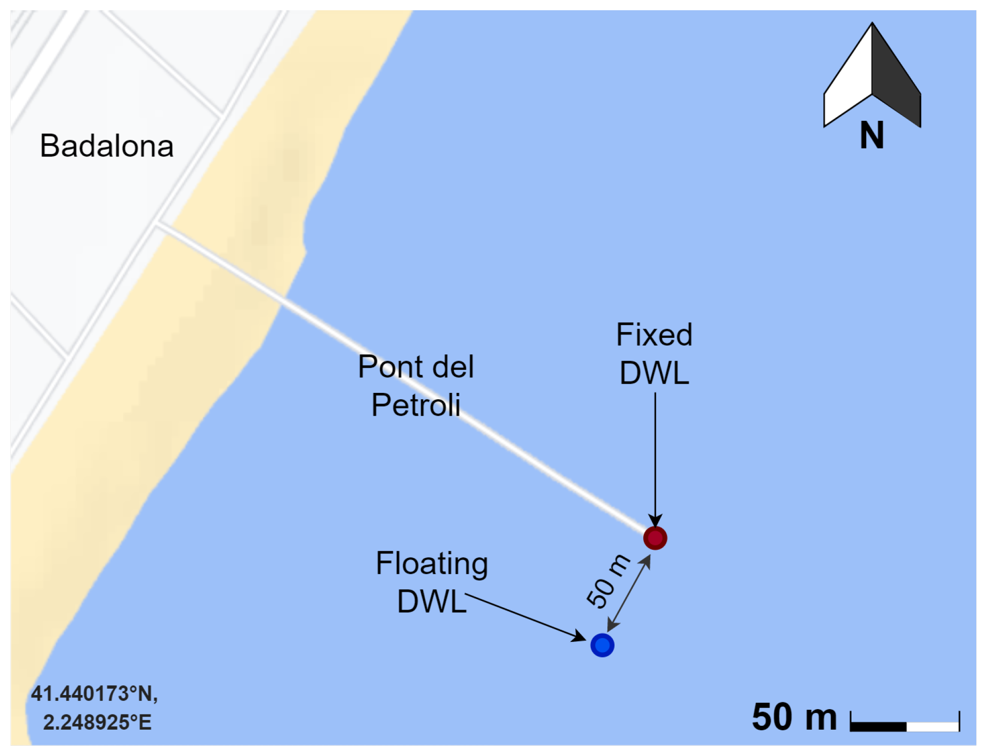
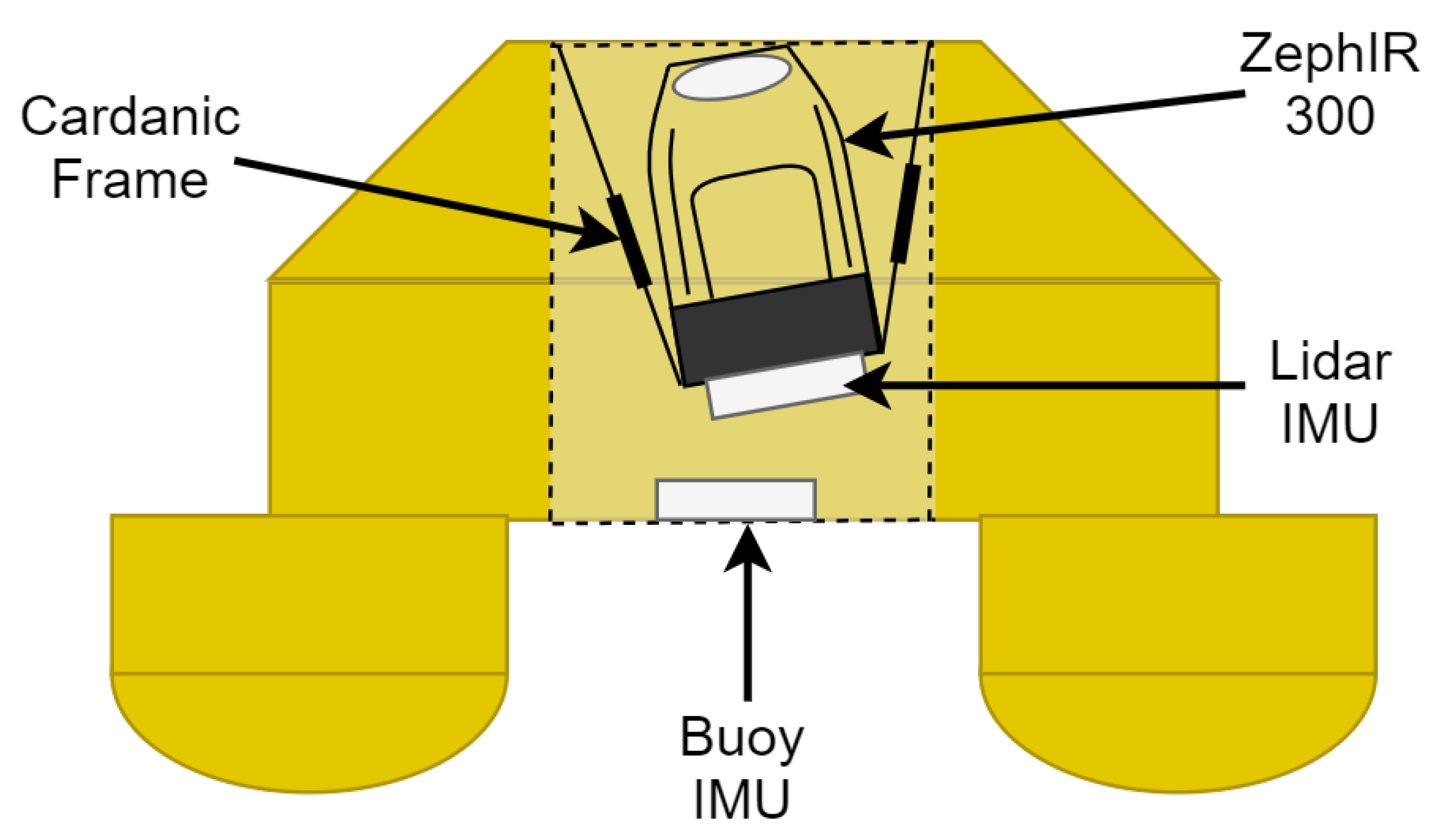
2.1. Instrumental Setup

In 2013, the Neptune project “proof-of-concept” LiDAR buoy validation campaign at PdP took place between May 24th and June 31st [21,27]. During the campaign, a proof-of-concept floating DWL buoy was compared against a fixed LiDAR, denoted “FDWL” and “fixed LiDAR”, respectively, in the following. Both the FDWL and the fixed LiDAR were ZephIR^TM 300 LiDARs. The fixed LiDAR was set up in stand-still configuration on PdP pier, as the reference device. The FDWL and the fixed LiDAR were located 50 m apart (see Figure 1). Both LiDARs were calibrated onshore, 1 m apart and over a period of 3 h, to ensure identical measurements on a 1 s and 10 min time basis. PdP is located on the coastline of Badalona (Barcelona, Spain), in the Barcelona metropolitan area. The experiment location surroundings are defined by an urban topology of low-height buildings (up to 20 m), which follow the coastline in the west and north cardinal directions, while the rest is defined by a sea-type topology.

The ZephIR 300 is a continuous-wave focused Doppler LiDAR manufactured by Zephir Ltd., United Kingdom (today ZX LiDARs^TM), which is prepared for offshore operation [28]. The device can measure the wind at user-defined heights between 10 m to 200 m, in steps of 1 m [29]. The LiDAR uses the VAD algorithm to retrieve the wind vector by measuring 50 LoSs at equally spaced azimuth angles (7.2-deg azimuth step between LoSs) along a conical scan of 30-deg aperture width from zenith. The ZephIR 300 can reach up to 1 scan/s when there is no LiDAR re-focusing required or CPU dead-time internal processes [29].

The FDWL was mounted on a proof-of-concept 3 m diameter buoy, designed as a prototype for offshore LiDAR operations. The buoy design was optimized for LiDAR measurements, as well as for tracking wave-induced motion on the device. The LiDAR was placed on a cardanic frame, aimed to keep the instrument still and to reduce the impact of buoy motion. The buoy was equipped with additional sensors, to measure different wind and sea parameters. Specifically, it hosted two MicroStrain 3DM-GX3-45 inertial measurement units (IMU), which combined a high-precision GPS antenna, an accelerometer, and a gyro. The first IMU (i.e., the LiDAR IMU) was located under the LiDAR bottom, and the second IMU (i.e., the buoy IMU) was located on the buoy structure bottom (see Figure 2), being able to measure the buoy and LiDAR attitude. During the campaign, different LiDAR measurement configurations were tested.

2.2. Basic Theoretical Definitions

The wind vector, $\mathit{U}$, is defined as a three-component vector formed by the HWS, WD (clockwise from north), and vertical wind speed (VWS), as

$$\mathit{U}=\left[\begin{array}{c}HWS\\ WD\\ VWS\end{array}\right].$$

(1)

In WE, a standard sampling period of 10 min was used. The mean wind conditions at this resolution were obtained by simply averaging the high-resolution (1 s) wind-vector components into a 10 min period. Thus, the mean HWS was computed as

$$\overline{HWS}=\frac{1}{N}\sum _{n=1}^{N}HW{S}_n,$$

(2)

where $HW{S}_n$ is the high-resolution HWS measurement and $N=600$ is the number of 1 s measurements in one minute.

We are also interested in the HWS variations, with respect to the mean HWS. This variability was measured by means of the TI, which is defined as

$$TI=\frac{{\sigma }_{HWS}}{\overline{HWS}},$$

(3)

where ${\sigma }_{HWS}$ is the 10 min HWS standard deviation. The standard deviation is defined as

$${\sigma }_{HWS}=\sqrt{\frac{1}{N-1}\sum _{n=1}^N(HW{S}_n-\overline{HWS})}.$$

(4)

2.3. The Estimation Viewpoint

The KF relies on two steps to estimate the hidden state-vector of the physical system under study: The prediction step and the innovation step [24].

The prediction step is defined by two equations, which are formulated in state-space notation as

$$\begin{array}{cc}\hfill {\mathit{x}}_{k|k-1}& =f\left({\mathit{x}}_{k-1|k-1}\right)+{\mathit{v}}_k,\hfill \end{array}$$

(5)

$$\begin{array}{cc}\hfill {\mathit{z}}_{k|k-1}& =h\left({\mathit{x}}_{k|k-1}\right)+{\mathit{n}}_k.\hfill \end{array}$$

(6)

The first equation is the prediction equation, in which ${\mathit{x}}_{k|k-1}$ is the hidden state-vector to be estimated, based on the previous state-vector estimate, ${\mathit{x}}_{k-1|k-1}$. Sub-indices $n|m$ denote estimation at the discrete time instant n, conditioned to all available information up to time m. Here, ${\mathit{x}}_{k|k-1}$ is the motion-free wind vector to be estimated, based on previous wind-vector estimations. $f(·)$ is the state-transition function predicting the state-vector at discrete time k, ${\mathit{x}}_{k|k-1}$, given previous knowledge of the state-vector, ${\mathit{x}}_{k-1|k-1}$; that is, $f(·)$ describes the stochastic wind model (to be found) that predicts the measured wind vector at the next time step from the wind vector at the previous one. ${\mathit{v}}_k$ is the process noise. The temporal resolution is the scan period (1 s approximately, see Section 2.4).

The second equation is the measurement equation, which estimates the present-time measurement, ${\mathit{z}}_{k|k-1}$, given the a priori state-vector, ${\mathit{x}}_{k|k-1}$, and motion information (to be further developed in Section 2.6), through the measurement function $h(·)$. In other words, the measurement function models the FDWL motion dynamics and estimates the expected motion-corrupted wind measurements, based on the a priori state-vector and IMU motion information vector $\mathit{M}$ (to be defined in Section 2.6). ${\mathit{n}}_k$ is the measurement noise.

On the other hand, the innovation step allows for the assimilation of the present-time measurement information into the a priori state-vector estimate through a projection gain (the so-called Kalman gain). Formally,

$${\widehat{\mathit{x}}}_{k|k}={\mathit{x}}_{k|k-1}+{\mathit{K}}_k({\mathit{z}}_k-{\mathit{z}}_{k|k-1}),$$

(7)

where ${\mathit{z}}_k$ is the wind-vector measurement and ${\mathit{K}}_k$ is the Kalman gain matrix. The latter relates the measurement estimation error, $\Delta \mathit{z}={\mathit{z}}_{k|k}-{\mathit{z}}_{k|k-1}$, to the a priori state-vector estimation error, $\Delta \mathit{x}={\mathit{x}}_{k|k}-{\mathit{x}}_{k|k-1}$.

To implement the UKF, both the state-transition wind model $f(.)$ and FDWL motion-dynamics measurement function $h(.)$ must be found. This is tackled in the following section.

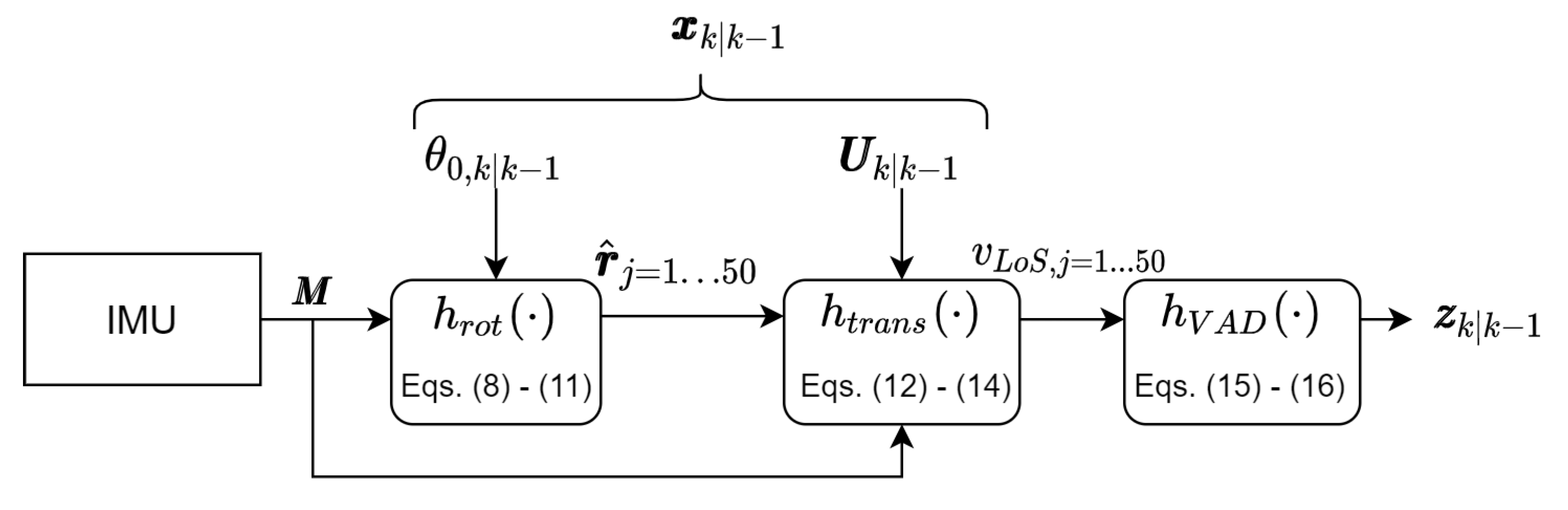
2.4. The Measurement Model: FDWL Motion

The wind vector is retrieved from the Doppler wind projection along the LoSs in the conical scan pattern by means of the VAD algorithm (see Section 2.4.3). In real operating conditions of the FDWL, sea-induced motion disturbs the conical scan, such that the pointing direction and measured radial velocities become affected by rotational and translational motion. In the motion-correction study by Kelberlau et al. [20], a complete geometrical description of the problem is thoroughly given. Next, we summarize and adapt information from this reference which are relevant to derive the measurement function $h(.)$ shown in Equation (6) above.

To describe the FDWL system, we first define the right-handed Cartesian XYZ “moving-body” coordinate system of the buoy and the north–east–down right-handed Cartesian NED “fixed” global frame of reference (see Figure 3). The latter is the inertial frame of reference in which the wind vector and FDWL motion are defined. Without external influence, the X, Y, and Z axes of the moving-body coordinate system are aligned with the north, east, and vertically down vectors of the fixed NED frame of reference. Wind, waves, and external forces cause translational motion in the N, E, and D directions (surge, sway, and heave, respectively), and rotational motion along the N, E, and D axes (roll, pitch, and yaw, respectively). We define $\widehat{x}$, $\widehat{y}$, and $\widehat{z}$ as unit vectors aligned with the X, Y, and Z axes of the moving-body coordinate system. On the other hand, $\widehat{n}$, $\widehat{e}$, and $\widehat{d}$ are defined as the unit vectors aligned with the north, east, and vertically down axes of the global NED frame of reference. $\widehat{h}$ is defined as the LiDAR beam direction before the prism deflection. The vector $\widehat{h}$ is defined as the opposite vector to $\widehat{z}$. The LoSs are measured in a cone of ${\varphi }_0$-deg width from $\widehat{h}$. Finally, we define ${\theta }_0$ as the LiDAR initial scan phase (i.e., the azimuth angle of the LiDAR pointing direction at the first LoS; denoted ${\widehat{r}}_1$), with respect to $\widehat{x}$ in the XY plane. During a scan, the LiDAR pointing direction $\widehat{r}$ ranges from $\theta =-{\theta }_0$ to $\theta =-{\theta }_0+360\times 1s$, with a fixed step $\Delta \theta$ between consecutive LoSs in a scan, which are denoted by ${\widehat{r}}_n$ and ${\widehat{r}}_{n+1}$, where n is the LoS number.

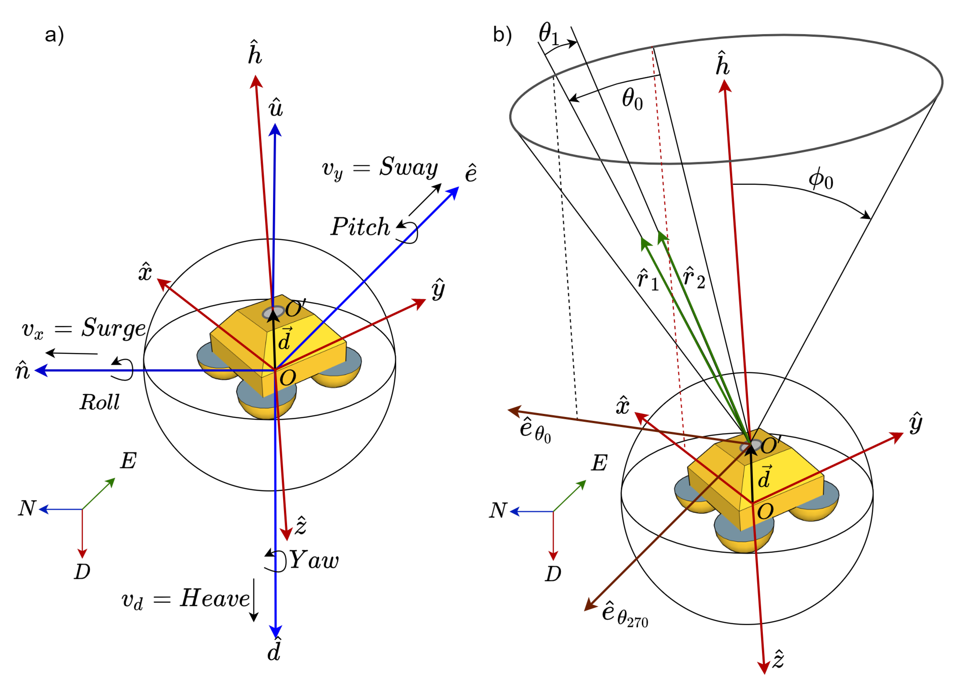
2.4.1. Rotational Motion

The rotational model (to be formulated as function $h_{rot}(·)$ in Section 2.6) computes the “true” LiDAR pointing direction vectors by means of a series of geometrical operations. Rotational motion affects the LiDAR pointing direction in each LoS, ${\widehat{r}}_n,n=1,\cdots ,50$. A series of chained vector rotations (refer to [20], Equations (5)–(12)) are needed to re-encounter $\widehat{r}$ in the NED reference frame (in the following, $\widehat{r}$ will be used as shorthand notation for the vector set ${\widehat{r}}_n,n=1,\cdots ,50$). This is derived next:

The Euler rotation matrix is used to express $\widehat{x}$, $\widehat{y}$, and $\widehat{z}$ in the NED frame of reference given roll, pitch, and yaw values ([20], Equations (5)–(7)). The unitary vector $\widehat{h}$ in the direction of the laser beam, before it is deflected by the LiDAR prism, is computed as ([20], Equation (8)):

$$\widehat{h}=-\widehat{z}.$$

(8)

${\widehat{e}}_{{\theta }_0}$, which denotes the vector in the direction of LiDAR heading in the N-E plane (i.e., the azimuth angle of ${\widehat{r}}_1$), is obtained by rotating $\widehat{x}$ along $\widehat{h}$ by $\theta$ deg, as:

$${\widehat{e}}_{{\theta }_1}=R(\widehat{h},\theta )·\widehat{x},$$

(9)

where $R(\widehat{h},\theta )$ is the rotation matrix about $\widehat{h}$$\theta$ degrees ([20], Equation (9)). Then, auxiliary vector ${\widehat{e}}_{{\theta }_{270}}$, defined as the unit vector perpendicular to ${\widehat{e}}_{{\theta }_0}$ in the N-E plane, is encountered as ([20], Equation (10)):

$${\widehat{e}}_{{\theta }_{270}}=\widehat{h}\times {\widehat{e}}_{{\theta }_0}.$$

(10)

Finally, the first LiDAR pointing direction $\widehat{r_1}$ can be expressed in the NED frame of reference by rotating $\widehat{h}$ by ${\varphi }_0$ deg along ${\widehat{e}}_{{\theta }_{270}}$, as:

$${\widehat{r}}_1=R({\widehat{e}}_{{\theta }_{270}},{\varphi }_0)·\widehat{h}.$$

(11)

The remaining LiDAR pointing directions in a scan, ${\widehat{r}}_n,n=2,\cdots ,50$ are obtained by changing the scan angle ${\theta }_0$ into ${\theta }_{n-1}$, with n as above.

2.4.2. Translational Motion

The translational model (formulated as function $h_{trans}(·)$ in Section 2.6) computes the set of 50 LiDAR-measured, LoS radial velocities during a scan, ${\mathit{v}}_{LoS}$. Translational motion also influences the measured LoS velocities. To study its effects, we need to account for all the velocity components at the position of the LiDAR scanning prism (origin of the scanning cone, $O^{\prime }$ in Figure 3). First, we define $\overrightarrow{d}$ as the distance vector between the origin of the NED coordinate system (O in Figure 3) and that of the scanning cone in the NED frame of reference ($O^{\prime }$ in Figure 3). The velocity experienced at measurement location $O^{\prime }$, $\overrightarrow{v_{lidar}}$, becomes influenced by both the translational velocities experienced by the LiDAR and rigid-body motion caused by the angular velocities. This composite effect can be expressed as ([20], Equation (14))

$$\overrightarrow{v_{lidar}}=\widehat{n}{v}_n+\widehat{e}{v}_e+\widehat{d}{v}_d+\left(\widehat{n}{\omega }_n\right)\times \overrightarrow{d}+\left(\widehat{e}{\omega }_e\right)\times \overrightarrow{d}+\left(\widehat{d}{\omega }_d\right)\times \overrightarrow{d},$$

(12)

where $v_n$, $v_e$, and $v_d$ are surge, sway, and heave motions, respectively, and ${\omega }_n$, ${\omega }_e$ and ${\omega }_d$ are roll, pitch, and yaw angular velocities, respectively.

Finally, the translational velocity contribution into a LoS ([20], Equation (15)) is the projection of $\overrightarrow{v_{lidar}}$ onto $\widehat{r}$ ([20], Equation (15)):

$$v_{LoS}=\widehat{r}·\overrightarrow{v_{lidar}}.$$

(13)

The radial velocity measured by the LiDAR along a LoS is encountered as the difference between the wind-vector projection over $\widehat{r}$ and $v_{LoS}$, as:

$$v_r=\overrightarrow{U}·\widehat{r}-v_{LoS}.$$

(14)

2.4.3. VAD Algorithm

The VAD model (formulated as $h_{VAD}(·)$ in Section 2.6) retrieves the wind vector $\mathit{U}$ from the measured LoS velocities, ${\mathit{v}}_{LoS}$. Assuming a uniform wind field, the measured radial wind, as a function of the azimuth LiDAR scan angle, takes the form of a cosine wave [26]. The VAD algorithm uses the least-squares method (LSQ) to fit a sinusoidal function to the measured radial velocities in the conical scan, $v_r$, at LoS azimuth angles $\varphi$. Formally,

$$v_r\left(\varphi \right)=|Acos(\varphi -B)+C|,$$

(15)

where A, B, and C are the LSQ solving variables, which yield the wind-vector information as:

$$\begin{array}{cc}\hfill HWS& =A/sin\left(\varphi \right),\hfill \\ \hfill WD& =B\pm 180deg,\hfill \\ \hfill VWS& =C/cos\left(\varphi \right).\hfill \end{array}$$

(16)

The sign ambiguity in the WD is due to the ZephIR 300 homodyne LiDAR detection, i.e., the LiDAR can only measure unsigned Doppler frequency shifts, which leads to 180-deg ambiguity in the WD retrieved by the VAD algorithm [26]. This ambiguity is resolved by means of the wind vane installed on the buoy.

2.5. State-Transition Model

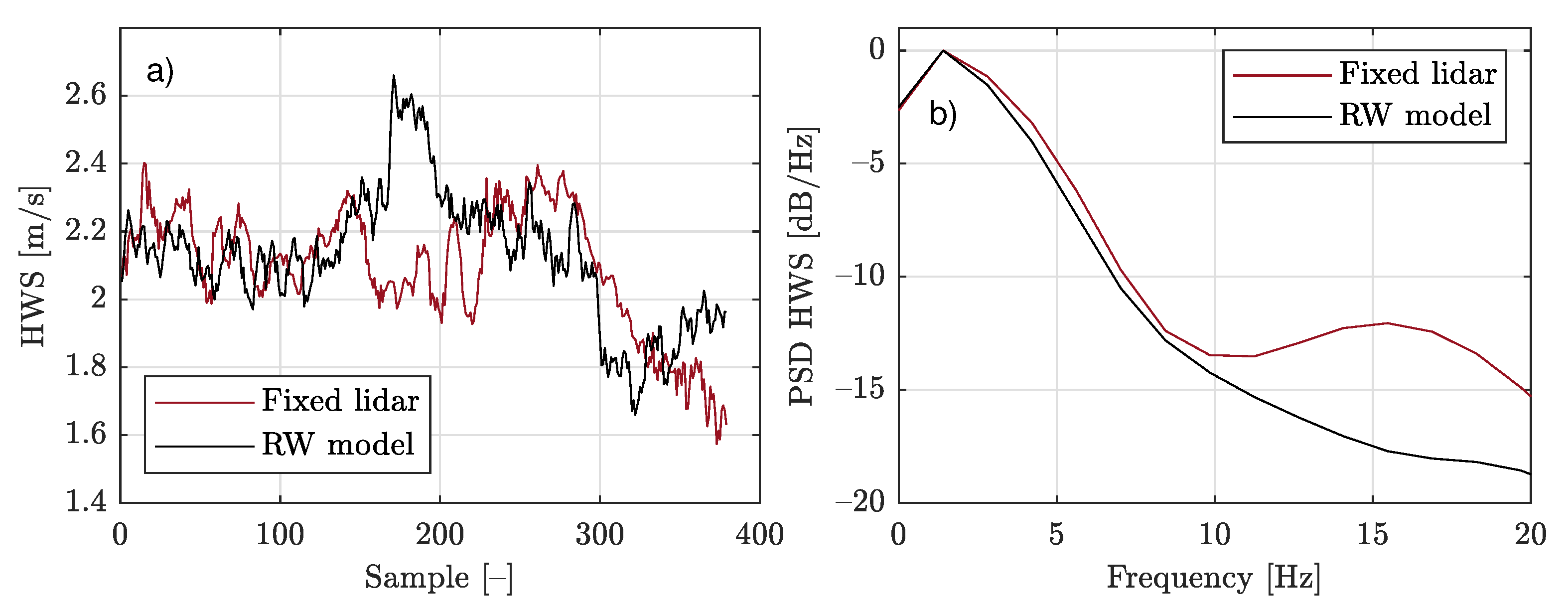
2.5.1. Wind Model

The LiDAR-retrieved wind vector is a non-stationary stochastic process dependent on the atmospheric conditions [30]. For instance, the wind field gusty nature causes high wind speed increments during short time periods [16]. Although physically rooted, advanced turbulent models describing the spectral tensor for atmospheric surface-layer turbulence [22] provide a refined solution, their application is hampered by their complexity and demand for computational resources. Instead, we propose a straightforward and oversimplified approach, in which the wind process is modelled as a random-walk (RW) stochastic process, in a similar fashion as what was used for the initial scan-phase model. It is formulated as:

$${\mathit{U}}_k={\mathit{U}}_{k-1}+{\mathit{ϵ}}_k,$$

(17)

where ${\mathit{ϵ}}_k$ is a random variable with zero-mean Gaussian distribution, $N(0,\sigma )$.

Figure 4 compares the HWS time-series estimated from the RW model (Equation (17)) to that measured by the fixed LiDAR. Figure 4a) demonstrates a similar dynamic range and process variability between both time-series, during most of the time. This is corroborated in Figure 4b), in terms of their associated Power Spectral Densities (PSD). Both PSDs were virtually coincident in the first spectral lobe (10 Hz cut off, −15 dB), indicating that RW modelling is a promising candidate for our estimation purposes. Discrepancies above 10 Hz were responsible for partial time-series tracking around sample nos. 150–200 in Figure 4a).

2.5.2. Initial Scan-Phase Model

The LiDAR initial scan phase, ${\theta }_0$, has great influence on the measurement error and, therefore, is of key importance for LiDAR motion correction [13]. However, ${\theta }_0$ is an undisclosed parameter from the manufacturer’s side, which needs to be estimated. In the motion-correction study by Gutiérrez-Antuñano et al. [13], ${\theta }_0$ is considered a random variable with uniform probability density from 0 to 360 deg. Based on this assumption, the LiDAR initial scan-phase process is modelled as a RW process, as:

$${\theta }_{0,k}={\theta }_{0,k-1}+{ϵ}_k,$$

(18)

where ${ϵ}_k$ is a uniform random variable in $[0,360)$ deg.

2.6. State-Space Formulation of the Problem

Once the measurement (Section 2.4) and state-transition models (Section 2.5) have been formulated, we aim to derive associated measurement and state-transition functions $h(.)$ and $f(.)$, respectively, in accordance with the state-space formulation presented in Section 2.3.

State-transition function $f(.)$.- To derive the state-transition function, first we considered the “clean” (i.e., motion-free) wind vector, ${\mathit{U}}_k$, which is to be estimated from the motion-corrupted wind vector ${\mathit{U}}_k^{FDWL}$ from the FDWL. The state-vector to be estimated, ${\mathit{x}}_{\mathit{k}}$, is formed by the clean wind vector at time k, ${\mathit{U}}_k$, and the LiDAR initial scan phase at that discrete time, ${\theta }_{0,k}$. This is formulated as

$${\mathit{x}}_k={\left[\begin{array}{cc}{\mathit{U}}_k^T& {\theta }_{0,k}\end{array}\right]}^T,$$

(19)

which using Equation (1), can be expanded to

$$\begin{array}{c}\hfill {\mathit{x}}_k={\left[\begin{array}{cccc}HW{S}_k& W{D}_k& VW{S}_k& {\theta }_{0,k}\end{array}\right]}^T.\end{array}$$

(20)

By inserting the state-vector Equation (20) above, along with the RW models for the wind and initial scan-phase processes (Equations (17) and (18), respectively) into prediction Equation (5), we obtain

$${\mathit{x}}_{k|k-1}=\mathit{I}·{\mathit{x}}_{k-1|k-1}+{\mathit{v}}_k,$$

(21)

where I is the identity matrix. This enables us to identify state-transition function $f(·)$, as:

$$f\left({\mathit{x}}_{k-1|k-1}\right)=\mathit{I}·{\mathit{x}}_{k-1|k-1}.$$

(22)

In Equation (22) above, the state-vector is a 4-component vector, estimated at each successive LiDAR scan (i.e., with approximately 1 s temporal resolution). Recall that sub-indices $n|m$ refer to estimation at discrete time n, based on past information up to discrete time m.

Measurement function $h(.)$—The measurement equation (Equation (6)) predicts the motion-corrupted wind-vector ${\mathit{z}}_{k|k-1}$ measured by the FDWL (i.e., the observation vector) from the estimated state-vector, ${\mathit{x}}_{k|k-1}$. The observation vector is written as

$${\mathit{z}}_k={\mathit{U}}_k^{FDWL}={[HW{S}_{FDWL},W{D}_{FDWL},VW{S}_{FDWL}]}^T,$$

(23)

where $HW{S}_{FDWL}$, $W{D}_{FDWL}$, and $VW{S}_{FDWL}$ are the FDWL measurements of HWS, WD, and VWS, respectively. ${\mathit{z}}_k$ is a 3-component vector computed at each successive time scan.

As the measurement function $h(·)$ is time variant depending on the attitude motion of the LiDAR, we define the motion block-vector ${\mathit{M}}_k$ describing the 6-DoF motion of the FDWL during a scan as:

$${\mathit{M}}_k=[{\mathit{R}}_k,{\mathit{P}}_k,{\mathit{Y}}_k,{\mathit{v}}_{\mathit{x}}k,{\mathit{v}}_{\mathit{y}}k,{\mathit{v}}_{\mathit{d}}k],$$

(24)

where ${\mathit{R}}_k$, ${\mathit{P}}_k$, ${\mathit{Y}}_k$, ${\mathit{v}}_{\mathit{x}}k$, ${\mathit{v}}_{\mathit{y}}k$, and ${\mathit{v}}_{\mathit{d}}k$ are the roll, pitch, yaw, surge, sway, and heave time-series measured by the IMU at 10 Hz temporal resolution and interpolated at 50 Hz. Numerically, the block-vector M is a 50 × 6 matrix, where each row is a LoS attitude measurement, and each column is an attitude parameter.

Assuming uniform wind flow during the LiDAR scan at time k, the motion-corrupted FDWL observations in a scan can be described by a set of three successive operations (Section 2.4, and refer to Figure 5):

(i)

retrieval of the motion-corrupted instantaneous LoS set, $\widehat{\mathit{r}}$;

(ii)

estimation of the associated LoS velocities, ${\mathit{v}}_{LoS}$; and

(iii)

VAD retrieval of the motion-corrupted observation wind vector, ${\mathit{z}}_{k|k-1}$;

where $\widehat{\mathit{r}}$ denotes the block-vector $[{\widehat{r}}_1,{\widehat{r}}_2,\cdots ,{\widehat{r}}_n]$, $n=1,\cdots ,50$, and each component represents the $n\mathrm{th}$ LoS unit vector (Figure 3).

Figure 5 block diagram depicts the filter measurement function $h(·)$ as a chain calculus process:

First, at each discrete time k, the 50 motion-corrupted LoSs during the scan ($[{\widehat{r}}_1,{\widehat{r}}_2,...,{\widehat{r}}_n]$, $n=1,\cdots ,50$) are computed by means of the geometrical operations presented in Section 2.4.1 (Equations (9)–(12)). This set of operations is denoted $h_{rot}(·)$ in Figure 5. The function $h_{rot}(·)$ computes the block-vector $\widehat{\mathit{r}}=[{\widehat{r}}_1,{\widehat{r}}_2,...,{\widehat{r}}_{50}]$ in the global NED frame of reference based on roll, pitch, and yaw instantaneous angles from attitude vector ${\mathit{M}}_k$ and predicted initial phase ${\theta }_{0,k|k-1}$ from the state-vector, ${\mathit{x}}_{k|k-1}$. Therefore, the block-vector $\widehat{\mathit{r}}$ can be written as

$$\widehat{\mathit{r}}=h_{rot}({\mathit{x}}_{k|k-1},{\mathit{M}}_k).$$

(25)

Second, the motion-corrupted LoS velocities at time k, ${\mathit{v}}_{LoS,k}$, are calculated through the set of operations described in Section 2.4.2 (Equations (12) and (13)), and denoted $h_{trans}(·)$ in Figure 5. Function $h_{trans}(·)$ computes this set of velocities given the predicted wind vector, ${\mathit{U}}_{k|k-1}$, the estimated LoS directions from the previous block, $\widehat{\mathit{r}}$, and by considering the influence of LiDAR translational and rigid-body motion information, through Equation (14) and Section 2.4.2, given ${\mathit{M}}_k$. Then, ${\mathit{v}}_{LoS,k}$ is obtained as

$${\mathit{v}}_{LoS,k}=h_{trans}({\mathit{x}}_{k|k-1},\mathit{M},\widehat{\mathit{r}}).$$

(26)

Third, the motion-corrupted VAD-retrieved wind vector ${\mathit{z}}_{k|k-1}$ is determined from the 50-LoS set of velocities, ${\mathit{v}}_{LoS,k}$, by means of the least-squares VAD algorithm presented in Section 2.4.3 (Equations (15) and (16)). The VAD algorithm is denoted by $h_{VAD}(·)$ in Figure 5. Hence,

$${\mathit{z}}_{k|k-1}=h_{VAD}\left({\mathit{v}}_{LoS,k}\right).$$

(27)

This chain calculus to compute measurement function $h(·)$ can be formulated as the composition of $h_{rot}(·)$, $h_{trans}(·)$, and $h_{VAD}(·)$ functions (through the so-called “chain rule”), as:

$$h(·)=h_{VAD}(·)\circ h_{trans}(·)\circ h_{rot}(·).$$

(28)

The time-variant observation model Equation (6) can be formulated as

$${\mathit{z}}_{k|k-1}=h({\mathit{x}}_{k|k-1},\mathit{M})+{\mathit{n}}_k.$$

(29)

2.7. Estimation of State- and Observation-Noise Covariance Matrices

To ensure convergent, unbiased estimates, the UKF must have a priori knowledge of both the process noise, ${\mathit{v}}_k$, and measurement noise, ${\mathit{n}}_k$. These are zero-mean, additive white Gaussian noise processes with covariances, ${\mathit{Q}}_k$ and ${\mathit{R}}_k$, respectively, which must be found.

The process-noise covariance matrix, ${\mathit{Q}}_k$, is defined as

$${\mathit{Q}}_k=E\left[{\mathit{v}}_k{\mathit{v}}_k^T\right].$$

(30)

Likewise, the measurement-noise covariance is defined as

$${\mathit{R}}_k=E\left[{\mathit{n}}_k{\mathit{n}}_k^T\right].$$

(31)

As the measurement function $h(.)$ is time variant with the LiDAR motion vector $\mathit{M}$, so is the measurement noise. Additionally, the wind statistical moments are not stationary, and the noise covariance matrices are difficult to accurately describe. Instead, we propose the adaptive estimation of these matrices based on statistical physical inference [31,32,33]. In this study, the Robust Adaptive UKF (RAUKF) [34] is chosen, due to its low computational requirements, fast convergence, and overall good performance to adaptively estimate the noise covariances. Moreover, the RAUKF uses a fault-detection mechanism to detect filter failure due to inaccurate estimation of the noise covariance matrices. When a fault is detected, $\mathit{Q}$ and $\mathit{R}$ are adjusted (see Appendix B for details).

In contrast to Equation (30), the RAUKF does not estimate $\mathit{Q}$ as the ensemble average of ${\mathit{v}}_k{\mathit{v}}_k^T$ [35,36]. A more straightforward approach is to estimate the matrix ${\mathit{Q}}_k$ instantaneously (i.e., at each discrete time k), using the approximation $E\left[{\mathit{v}}_k{\mathit{v}}_k^T\right]$, and to balance it with previous estimates. As a further refinement, the RAUKF dynamically adjusts ${\widehat{\mathit{Q}}}_k$ by blending present and past estimates of the covariance matrix through a forgetting factor, $\lambda$, as:

$${\widehat{\mathit{Q}}}_k=(1-\lambda ){\widehat{\mathit{Q}}}_{k-1}+\lambda {\mathit{v}}_k{\mathit{v}}_k^T.$$

(32)

The RAUKF uses similar procedure as for ${\widehat{\mathit{Q}}}_k$, to compute the instantaneous estimations of ${\mathit{R}}_k$ through a forgetting factor $\delta$, as:

$${\widehat{\mathit{R}}}_k=(1-\delta ){\widehat{\mathit{R}}}_{k-1}+\delta {\mathit{n}}_k{\mathit{n}}_k^T.$$

(33)

A similar memory-fading procedure has been used in the radar application of the filter for atmospheric boundary layer height estimation [37]. In practice, factors in the range 0.1–0.2 provided convergent, unbiased results, as shown in Section 3.

2.8. Filter Initialization

The UKF initial space vector takes the form

$${\widehat{\mathit{x}}}_0={[{\mathit{U}}_0^{proxy},{\theta }_{0,0}]}^T,$$

(34)

where ${\mathit{U}}_0^{proxy}$ is the “proxy” wind time-series and ${\theta }_{0,0}$ is initial scan phase, ${\theta }_0$, at time $k=0$.

To initialize the filter, a 10 min length, moving-average time-series [21] of the first 1 s-resolution wind measurements (the so-called “proxy” time-series, ${\mathit{U}}_k^{proxy}$) is computed. The window length chosen is the wave period over the 10 min series, which is estimated by means of the L-dB method [38] (other wave-period estimation methods in the literature [39,40] yielded virtually identical results). The wind component of the state-vector is initialized by retaining the first-time sample of the proxy wind, ${\mathit{U}}_k^{proxy}$. The initial scan-phase component of the state-vector is initialized with a random value between 0 and 360 deg, as dictated by the assumption of the a priori unknown uniform phase distribution.

The state-noise covariance matrix is linked to RW process noise ${\mathit{v}}_k$ (Equation (5)). For simplicity, this matrix is assumed to be diagonal. At time $k=0$, this matrix is written as

$${\mathit{Q}}_0=diag\left(\left[\begin{array}{cccc}{\sigma }_{HWS}^2& {\sigma }_{WD}^2& {\sigma }_{VWS}^2& {\sigma }_{{\theta }_0}^2,\end{array}\right]\right),$$

(35)

where each component represents a variance.

As a RW process is characterized at each discrete time by incremental/detrimental random steps away from the previous value of the variable, ${\sigma }_{HWS}^2$, ${\sigma }_{WD}^2$, and ${\sigma }_{VWS}^2$ are estimated as the variance of difference between consecutive samples. For example, ${\sigma }_{HWS}^2$ is calculated from ${\mathit{U}}^{proxy}$ as

$${\sigma }_{HWS}^2=E\left[{(HW{S}_k^{proxy}-HW{S}_{k-1}^{proxy})}^2\right],$$

(36)

where $E(.)$ is the expectancy operator (in practice, a 10 min window average). Process noise ${\theta }_0$ is initialized with the noise variance of a uniform distribution from 0 to 360 deg as

$${\sigma }_{{\theta }_0}^2=\frac{{(b-a)}^2}{12}=\frac{{360}^2}{12},$$

(37)

where $a=0$ and $b=360$ deg are the lower and upper limits of the uniform distribution, respectively.

The measurement-noise covariance matrix at initial time, $k=0$, is formulated as

$${\mathit{R}}_0=diag\left(\left[\begin{array}{ccc}{\sigma }_{R,HWS}^2& {\sigma }_{R,WD}^2& {\sigma }_{R,VWS}^2\end{array}\right]\right),$$

(38)

where the subscript R is a remainder of covariance matrix ${\mathit{R}}_k$ and ${\sigma }_{R,i}$, $i=HWS,WD,VWS$ is the estimated measurement-noise standard deviation for each of the variables. We used ${\sigma }_{R,HWS}=0.05$ m/s, ${\sigma }_{R,WD}=50$ deg, and ${\sigma }_{R,VWS}=0.025$ m/s for the experimental data of Section 3. These measurement-noise standard deviations were roughly estimated from the 10 min proxy wind time-series, ${\mathit{U}}_k^{proxy}$, used to initialize the filter. These values were deliberately low, to ensure the smooth start-up of the filter, hence preventing divergence.

Finally, the a priori error covariance matrix, ${\widehat{\mathit{P}}}_0^{xx}$, is initialized as

$${\mathit{P}}_0^{-}={\mathit{Q}}_0,$$

(39)

which indicates that the user’s expected a priori error during initialization is comparable to the state-noise “nervousness” of the filter, ${\mathit{Q}}_0$.

3. Results

The motion-compensation algorithm was tested on the PdP experimental campaign by comparing the FDWL with reference to the fixed LiDAR. This is discussed in the following:

3.1. Data Set

The data set used for validation of the motion-correction algorithm comprised data from 6 to 30 June of 2013, with both LiDARs measuring at a fixed height of 100 m; specifically, (i) wind-LiDAR data from the FDWL, (ii) FDWL internal status parameters, and (iii) 6-DoF motion measurements by two IMUs, one on the LiDAR instrument (“lidar IMU” in what follows) and another on the buoy (“buoy IMU”), were used.

Lidar internal status parameters were available, to assess the LiDAR status as well as to ensure the quality of the VAD-retrieved wind-vector measurements. These parameters include the spatial variation (SV), backscatter, and other system parameters. The SV parameter is a LiDAR internal parameter representing the turbulence intensity of the variation degree of the radial wind speeds (LoS) within the circle of scan of the LiDAR [21]. The SV can be understood as a goodness-of-fit parameter of the VAD algorithm which is used to retrieve the wind vector at a given height [26,41]. By experiment, Gutiérrez-Antuñano et al. [21] showed strong correlation between the wind TI and the SV values measured by a fixed ZephIR 300 LiDAR at 100 m in height (SV = 0.02 was approximately related to TI = 5% and SV = 0.1 to TI = 30% therein). The backscatter coefficient is an internal dimensionless parameter indicative of the intensity of the backscattered light return. By experiment, a backscatter threshold of 0.1 is reported in [42] to distinguish between normal and low signal LiDAR returns.

Regarding the IMU data used for motion compensation, each of the IMUs was used for a different purpose: On one hand, the LiDAR IMU was used to measure rotational motion, as the LiDAR was mounted on the cardanic frame in such a way that its rotation center coincided with the LiDAR scan cone apex (location of the scanning prism; point O in Figure 3). On the other hand, the buoy IMU was used to measure translational motion.

3.2. Data Filtering

Lidar-measured data from both the fixed and FDWLs required outlier removal, which encompassed 999X values (a label for system measurement error), too-high wind speed, and rain-flagged data.

The ZephIR 300 LiDAR has a wind measurement range of 1–80 m/s [43]. In high-motion scenarios, wind measurements by the FDWL exhibited high variances as compared to the mean HWS. Ten-minute time-series with a HWS mean lower than 2.5 m/s were removed, to ensure reliable instantaneous HWS measurements [13]. Complex-terrain effects also cause non-negligible effects on the wind flow variability, which may well invalidate the assumption of uniform wind flow during the LiDAR scan [44]. Thus, metropolitan buildings along the coastline cause high spatial variability on the wind field [45], which demonstrates as a non-uniform wind vector along the LiDAR scanning cone. On the other hand, winds blowing from sea to land exhibit higher spatial homogeneity, which leads to more reliable LiDAR measurements. Following Section 3.1, 1-s data with SV greater than 0.2, which were indicative of spatially non-homogeneous winds, were filtered out. Similarly, data with associated backscatter coefficients smaller than a threshold of 0.02, which is indicative of LiDAR measurements with very low signal return, were rejected.

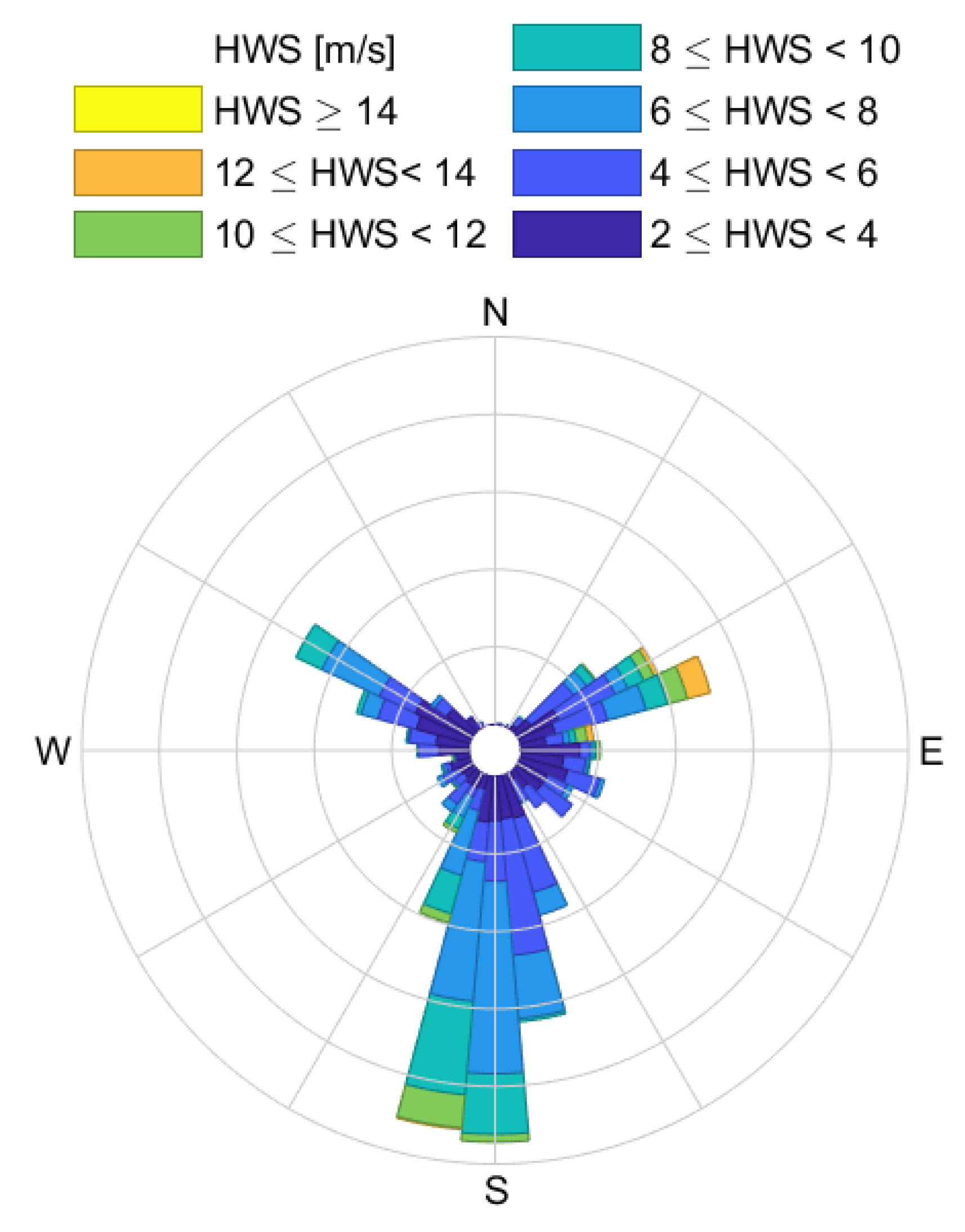
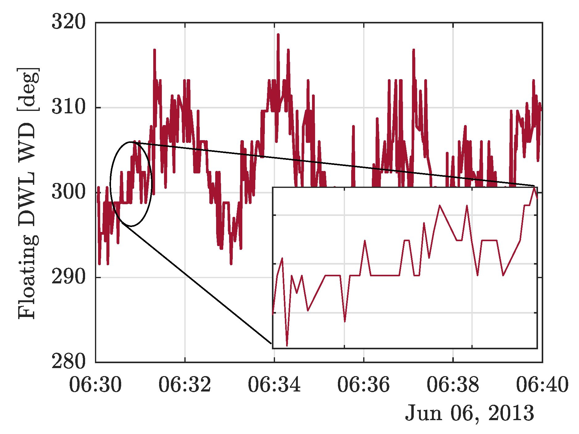
3.3. Campaign Overview

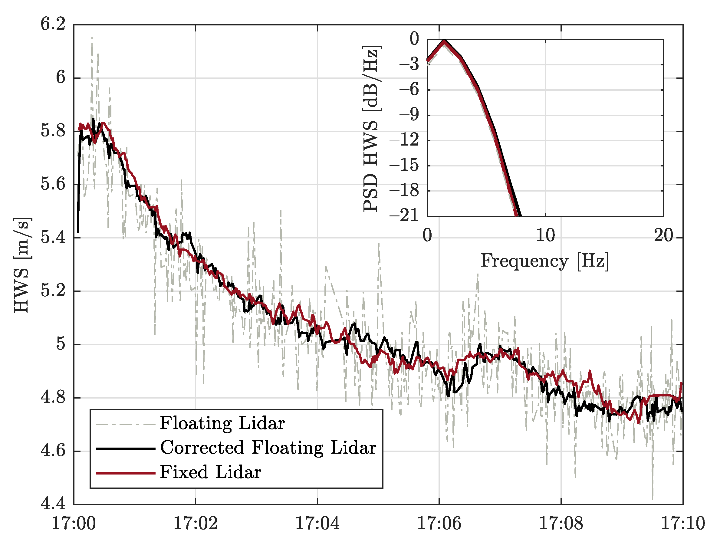
During the measurement period (6–30 June 2013), the surface layer was dominated by local thermal winds hardly rising above 15 m/s at 100 m in height [21]. The observed HWS in this period ranged from 1 m/s to 15 m/s, with three predominant WDs: North East (NE), North West (NW) and South (S); see Figure 6.

During the night, the wind was light, coming predominantly from the urban area (NW), showing low HWS values with high turbulence and spatial variability. During the day, the atmosphere was dominated by winds coming from the sea towards land (S and NE), with higher HWS and lower turbulence.

Both the fixed- and floating-lidar 10 min WD time-series showed unexpected high noise (roughly about ±5-deg uncertainty in Figure 7). This phenomenon is called “granularity” herein, and was caused by a LiDAR flaw. This issue was solved in a later manufacturing series of the instrument [10].

3.4. UKF Results

Low/High-turbulence scenario analysis.—The filter was applied to the campaign data set described in Section 3.3. The filter converged in most cases, achieving successful motion correction when compared to the reference fixed LiDAR. Divergent cases (accounting for less than 0.5% of the statistical sample) were attributable to strong wind shears, which motivated retuning of the measurement-noise variance settings in Equation (38).

Figure 8 shows a low-turbulence case example, comparing a FDWL HWS measurement time-series with and without correction against the reference fixed-LiDAR time-series. Besides evident filter convergence, the motion-corrected HWS time-series matched almost ideally that of the reference LiDAR. The motion-induced error was greatly reduced from 0.14 m/s to 0.05 m/s RMSE, thus achieving good performance. When analyzing the PSD of these three time-series (see inset), it emerged that the RW model was able to emulate the wind process with high accuracy, up to some 21 dB roll-off at 7 Hz. However, the high-frequency components below −30 dB, which were not as relevant, were underestimated (data not shown).

Underestimation of frequency components may lead to motion over-correction by the UKF in high variance scenarios, as illustrated in Figure 9. It can be observed that the motion-corrected FDWL and fixed-LiDAR temporal series only partially matched each other. Spectral analysis underlined differences between the HWS PSDs (red and black traces), being as high as 5 dB at low frequencies (0 to 5 Hz) and increasing to ≃10 dB at high frequencies (5 to 20 Hz). This is a limitation of the used RW wind model, which was not able to emulate the high-frequency components of the wind spectrum. Consequently, the filter assimilated the wind model error as a measurement error, which led to biased estimations at specific times in Figure 9. Regarding 10-min WD estimation in either high-or low-variance scenarios (counterparts of Figure 8 and Figure 9, respectively, data not shown), the filter was able to retrieve the yaw-error-free WD with a RMSE as low as roughly 5 deg for both the high- and low-variance cases. Regarding the so-called 1-s WD estimation, the “granularity” effect showed up in the retrieved time-series in similar fashion as for the retrieved HWS.

Overall campaign analysis.- With a view to assess the overall filter performance, the TIs measured by the FDWL during the PdP campaign (25 days, 1875 records) with and without correction ($T{I}_{float.,corr.}$ and $T{I}_{float.}$, respectively) were compared to the TI measured by the fixed LiDAR ($T{I}_{fixed}$). In the context of WE, the typical temporal resolution of wind-related data products is 10 min; thus, the comparison was carried out at 10 min temporal resolution. To carry out this comparison, different statistical indicators were considered: (i) The determination coefficient ($R^2$), (ii) RMSE, and (iii) mean deviation (MD).

The RMSE for a sample of N motion-corrected measurements is defined as

$$RMSE=\sqrt{\frac{{\sum }_n^N{(T{I}_{float.,corr.}-T{I}_{fixed})}^2}{N}},$$

(40)

and the MD is defined as

$$MD=\frac{{\sum }_n^{N}T{I}_{float.,corr.}-T{I}_{fixed}}{N}.$$

(41)

The MD accounts for the systematic error in the LiDAR-measured TI (equivalently, HWS standard deviation) caused by wave-induced motion [9,46]. The RMSE and MD definitional formulae to compare FDWL uncorrected measurements to fixed-LiDAR measurements are analogous to Equations (40) and (41) above, by changing $T{I}_{float.,corr}$ to $T{I}_{float.}$.

The scatter plot shown in Figure 10 compares the TI measured by the FDWL (with and without correction) against the TI measured by the fixed LiDAR. Without correction, most of the $T{I}_{floating}$ values fell below the ideal 1:1 line. This was because buoy motion added an apparent variance to the HWS measurements, which increased the LiDAR-measured turbulence. The linear regression (LR, red dashed-dot line) offset of −0.0185 indicated the amount of added turbulence [14]. The LR slope of 1.0358, which is virtually identical to the ideal unity slope, indicates that the apparent turbulence equally affected all HWS measurements.

Regarding the motion-corrected TI measurements (black dots), the scatter points lay closer to the ideal 1:1 line, as demonstrated by an LR offset as low as 0.0032. This represented an 83% reduction factor, in comparison to the uncorrected measurements (offset term equal to 0.0185), and very small over-correction from the UKF side.

Scatter points away from the ideal 1:1 are a consequence of different filter model limitations: First, the LiDAR initial scan-phase model (Section 2.5.2) was unknown, the proposed RW models being only a reasonable rough approximation. Second, the retrieved WD by any of the two LiDAR instruments showed the so-called “granularity” issue, which accounted for uncertainties of some ± 5 degrees (see Section 3.3), and which could have well led to inaccurate correction by the UKF. Finally, in Figure 10, we did not include the start-up period of the filter, in which the noise covariance matrices are still not well-estimated. Third, a more homogeneous terrain experimental scenario should be used. FDWLs are conceived for open-sea environments, and the motion-correction should be tested in these scenarios.

The overall campaign results demonstrated the good performance of the filter in reducing the apparent TI caused by buoy motion. All statistical indicators (see

Table 1. Statistical indicators evaluating the comparison between FDWL (with and without correction) and fixed LiDAR TI measurements at the 10 min level.

	Uncorrected	Motion-Corrected	WD Filtered Motion-Corrected
$R^2$	0.85	0.90	0.93
RMSE	2.01%	1.01%	0.86%
MD	−1.70%	0.29%	0.36%

) improved: (i) the coefficient of determination, $R^2$, rose from 0.85 (without compensation) to 0.90 (with compensation); (ii) the RMSE reduced from 2.01% (without) to 1.01% (with); and (iii) the MD increased from −1.70% to 0.29%, accounting for an 83% factor improvement.

However, closer inspection of the measurement setup warrants some comments, regarding the statistical indicators shown: First, the floating and the fixed LiDARs were located 50 m apart and, although they measured similar wind conditions, the instantaneous wind measurements were not the same. This would have required setting up two LiDARs co-located at the same place. Specifically, winds blowing from/to the urban area (WDs between 270 and 330 deg, and between 90 and 150 deg, respectively) experienced higher spatial and temporal variation, due to terrain roughness [45], which led to different HWS time-series being measured by the LiDARs (see Section 3.3).

According to Taylor’s frozen-atmosphere theory [47], turbulent eddies transported by the mean wind hold their properties as if they were “frozen”, such that two points aligned with the mean WD will observe the same wind stochastic realization, with a time delay. This delay is inversely proportional to the mean HWS. The floating and the fixed LiDARs were mainly aligned along the north-south direction and, therefore, only measurement records with WDs within 180±30 deg will be considered for further, enhanced statistical analysis. The maximum delay measured between the two LiDARs was 25 s, which is a negligible value, compared to the measurement period of 10 min.

After the WD was filtered, as indicated, the statistical indicators improved, as shown in the third column of Table 1. The coefficient of determination increased to 0.93 and the RMSE decreased to 0.86%. The small increase in MD (0.36%) was not significant, on account of the approximate WD filtering procedure.

4. Conclusions

An adaptive method for 6-DoF motion compensation of ZephIR 300 FDWL wind measurements was presented in this paper. The RAUKF algorithm proved to be capable of correcting the motion-induced error in the retrieved HWS (Figure 8) and TI (Figure 10), without accessing LiDAR LoS velocity measurements, which is undisclosed information from the manufacturer’s side for most of the commercial continuous-wave wind LiDARs. To the best of our knowledge, this is a key state-of-the-art contribution of this work.

The proposed solution departed from the FDWL motion dynamics study [20] and the well-known VAD wind-retrieval algorithm, to derive an ad-hoc state-space formulation of the problem from the point of view of control theory, using an UKF and stochastic modelling. The state-vector transition model relied on a RW model to describe the unknown motion-corrected wind vector (to be found) and blind LiDAR initial scan phase. The measurement model was time variant and combined the buoy’s 6-DoF IMU information with the filter’s estimated motion-corrected wind vector, to predict the FDWL motion-corrupted wind measurements. The recursive loop of the filter, combined with run-time estimation of the state-vector and measurement-noise covariance matrices, ensured successful and convergent results.

The methodology was validated using the experimental data collected during a PdP measurement campaign in Barcelona, using a fixed LiDAR on the PdP pier as the reference instrument. To quantitatively assess filter performance, the 10 min TI measured by the FDWL with and without correction was compared to the TI measured by the reference LiDAR. Wind measurements were also WD screened, to ensure the validity of Taylor’s frozen-atmosphere assumption along the connecting line between the two LiDARs. All statistical indicators showed significant improvement Table 1: MD improved from −1.60% (without correction) to 0.36% (with correction), the RMSE improved from 1.9% to 0.86%, and the determination coefficient ($R^2$) increased from 0.86 to 0.93. Linear regression between floating- and fixed-TI measurements showed an offset equal to the apparent motion-induced TI added; which, upon correction by the filter, was virtually removed.

A limitation of the filter was its underestimation of the high-frequency components (i.e., fast transients) when comparing floating-lidar HWS temporal series with reference to fixed-LiDAR ones. This was due to the oversimplified RW wind model used. Notwithstanding the overall improvement in all the statistical indicators shown, a few outliers departed from the ideal 1:1 line between the motion-corrected and fixed-LiDAR TI observations. We hypothesize that this may be due to the filter start-up time (about 60 s before stable tracking condition is reached), as well as the so-called “granularity” effect in the LiDAR-retrieved WD.

All in all, the RAUKF was demonstrated to be an effective tool for 6-DoF motion correction of FDWL measurements and accurate TI measurements. Furthermore, the recursive operation of the filter allows room for stand-alone, nearly real-time correction of FDWL measurements.

References

1. Global Wind Energy Council. Global Wind Report 2018; Technical Report; Global Wind Energy Council: Brussels, Belgium, 2019. [Google Scholar]
2. Barthelmie, R.; Courtney, M.; Højstrup, J.; Larsen, S. Meteorological aspects of offshore wind energy: Observations from the Vindeby wind farm. J. Wind Eng. Ind. Aerodyn. 1996, 62, 191–211. [Google Scholar] [CrossRef]
3. Offshore Wind in Europe Key Trends and Statistics 2019; Technical Report; WindEurope: Brussels, Belgium, 2020.
4. Timmons, D. 25 - Optimal Renewable Energy Systems: Minimizing the Cost of Intermittent Sources and Energy Storage. In A Comprehensive Guide to Solar Energy Systems; Letcher, T.M., Fthenakis, V.M., Eds.; Academic Press: Cambridge, MA, USA, 2018; pp. 485–504. [Google Scholar] [CrossRef]
5. Carbon Trust. Carbon Trust Offshore Wind Accelerator Roadmap for the Commercial Acceptance of Floating LIDAR Technology; Technical Report; Carbon Trust: London, UK, 2013. [Google Scholar]
6. Peña, A.; Hasager, C.; Lange, J.; Anger, J.; Badger, M.; Bingöl, F.; Bischoff, O.; Cariou, J.P.; Dunne, F.; Emeis, S.; et al. Remote Sensing for Wind Energy; DTU Wind Energy: Roskilde, Denmark, 2013. [Google Scholar]
7. Sathe, A.; Mann, J. A review of turbulence measurements using ground-based wind lidars. Atmos. Meas. Tech. 2013, 6, 3147–3167. [Google Scholar] [CrossRef] [Green Version]
8. Berger, R. Offshore Wind toward 2020: On the Pathway to Cost Competitiveness; Technical Report; Roland Berger: Munich, Germany, 2013. [Google Scholar]
9. Gutiérrez, M.A.; Tiana-Alsina, J.; Bischoff, O.; Cateura, J.; Rocadenbosch, F. Performance evaluation of a floating Doppler wind lidar buoy in mediterranean near-shore conditions. In Proceedings of the 2015 IEEE International Geoscience and Remote Sensing Symposium (IGARSS), Milan, Italy, 26–31 July 2015; pp. 2147–2150. [Google Scholar] [CrossRef]
10. Gutierrez-Antunano, M.A.; Tiana-Alsina, J.; Rocadenbosch, F.; Sospedra, J.; Aghabi, R.; Gonzalez-Marco, D. A wind-lidar buoy for offshore wind measurements: First commissioning test-phase results. In Proceedings of the 2017 IEEE International Geoscience and Remote Sensing Symposium (IGARSS-2017), Fort Worth, TX, USA, 23–28 July 2017; IEEE: Fort Worth, TX, USA, 2017; pp. 1607–1610. [Google Scholar] [CrossRef]
11. Schuon, F.; González, D.; Rocadenbosch, F.; Bischoff, O.; Jané, R. KIC InnoEnergy Project Neptune: Development of a Floating LiDAR Buoy for Wind, Wave and Current Measurements. In Proceedings of the DEWEK 2012 German Wind Energy Conference, Bremen, Germany, 19–20 May 2012. [Google Scholar]
12. Mathisen, J.P. Measurement of wind profile with a buoy mounted lidar. Energy Procedia 2013, 30, 12. [Google Scholar]
13. Gutiérrez-Antuñano, M.; Tiana-Alsina, J.; Salcedo, A.; Rocadenbosch, F. Estimation of the Motion-Induced Horizontal-Wind-Speed Standard Deviation in an Offshore Doppler Lidar. Remote Sens. 2018, 10, 2037. [Google Scholar] [CrossRef] [Green Version]
14. Salcedo-Bosch, A.; Gutierrez-Antunano, M.A.; Tiana-Alsina, J.; Rocadenbosch, F. Floating Doppler Wind Lidar Measurement of Wind Turbulence: A Cluster Analysis. In Proceedings of the 2020 IEEE International Geoscience and Remote Sensing Symposium (IGARSS-2020), Waikoloa, HI, USA, 26 September–2 October 2020. [Google Scholar]
15. Courtney, M.S.; Hasager, C.B. Chapter 4: Remote sensing technologies for measuring offshore wind. In Offshore Wind Farms; Elsevier: Amsterdam, The Netherlands, 2016; pp. 59–82. [Google Scholar]
16. Mücke, T.; Kleinhans, D.; Peinke, J. Atmospheric turbulence and its influence on the alternating loads on wind turbines. Wind Energy 2011, 14, 301–316. [Google Scholar] [CrossRef]
17. Gottschall, J.; Gribben, B.; Stein, D.; Würth, I. Floating lidar as an advanced offshore wind speed measurement technique: Current technology status and gap analysis in regard to full maturity. Wiley Interdiscip. Rev. Energy Environ. 2017, 6, e250. [Google Scholar] [CrossRef]
18. Gottschall, J.; Wolken-Möhlmann, G.; Lange, B. About offshore resource assessment with floating lidars with special respect to turbulence and extreme events. J. Phys. Conf. Ser. 2014, 555, 12–43. [Google Scholar] [CrossRef]
19. Tiana-Alsina, J.; Rocadenbosch, F.; Gutierrez-Antunano, M.A. Vertical Azimuth Display simulator for wind-Doppler lidar error assessment. In Proceedings of the 2017 IEEE International Geoscience and Remote Sensing Symposium (IGARSS), Fort Worth, TX, USA, 23–28 July 2017; pp. 1614–1617. [Google Scholar] [CrossRef] [Green Version]
20. Kelberlau, F.; Neshaug, V.; Lønseth, L.; Bracchi, T.; Mann, J. Taking the Motion out of Floating Lidar: Turbulence Intensity Estimates with a Continuous-Wave Wind Lidar. Remote Sens. 2020, 12, 898. [Google Scholar] [CrossRef] [Green Version]
21. Gutiérrez-Antuñano, M.A.; Tiana-Alsina, J.; Rocadenbosch, F. Performance evaluation of a floating lidar buoy in nearshore conditions. Wind Energy 2017, 20, 1711–1726. [Google Scholar] [CrossRef] [Green Version]
22. Mann, J. Wind field simulation. Probabilistic Eng. Mech. 1998, 13, 269–282. [Google Scholar] [CrossRef]
23. Brown, B.G.; Katz, R.W.; Murphy, A.H. Time series models to simulate and forecast wind speed and wind power. J. Appl. Meteorol. Climatol. 1984, 23, 1184–1195. [Google Scholar] [CrossRef]
24. Rodgers, C.D. Inverse Methods for Atmospheric Sounding: Theory and Practice; Series on Atmospheric, Oceanic and Planetary Physics; World Scientific: Singapore, 2004; Volume 2. [Google Scholar]
25. Robert Grover, R.; Hwang, P.Y.C. Introduction to Random Signals and Kalman Filtering: With MATLAB Exercises, 4th ed.; Wiley: Hoboken, NJ, USA, 2012. [Google Scholar]
26. Slinger, C.; Harris, M. Introduction to Continuous-Wave Doppler Lidar. Available online: http://breeze.colorado.edu/ftp/RSWE/Chris_Slinger.pdf (accessed on 21 July 2021).
27. Sospedra, J.; Cateura, J.; Puigdefàbregas, J. Novel multipurpose buoy for offshore wind profile measurements EOLOS platform faces validation at ijmuiden offshore metmast. Sea Technol. 2015, 56, 25–28. [Google Scholar]
28. ZX Lidars. ZX 300M—Offshore Wind Measurements from Vertical Profiling Lidar; ZX Lidars: Ledbury, UK, 2021. [Google Scholar]
29. Pitter, M.; Burin des Roziers, E.; Medley, J.; Mangat, M.; Slinger, C.; Harris, M. Performance Stability of Zephir in High Motion Enviroments: Floating and Turbine Mounted; Technical Report; ZephIR: Ledbury, UK, 2014. [Google Scholar]
30. Smith, D.A.; Mehta, K.C. Investigation of stationary and nonstationary wind data using classical Box-Jenkins models. J. Wind Eng. Ind. Aerodyn. 1993, 49, 319–328. [Google Scholar] [CrossRef]
31. Davari, N.; Gholami, A. An Asynchronous Adaptive Direct Kalman Filter Algorithm to Improve Underwater Navigation System Performance. IEEE Sens. J. 2017, 17, 1061–1068. [Google Scholar] [CrossRef]
32. Koivisto, M.; Seppänen, J.; Mellin, I.; Ekström, J.; Millar, J.; Mammarella, I.; Komppula, M.; Lehtonen, M. Wind speed modeling using a vector autoregressive process with a time-dependent intercept term. Int. J. Electr. Power Energy Syst. 2016, 77, 91–99. [Google Scholar] [CrossRef]
33. Li, W.; Sun, S.; Jia, Y.; Du, J. Robust unscented Kalman filter with adaptation of process and measurement noise covariances. Digit. Signal Process. 2016, 48, 93–103. [Google Scholar] [CrossRef]
34. Zheng, B.; Fu, P.; Li, B.; Yuan, X. A Robust Adaptive Unscented Kalman Filter for Nonlinear Estimation with Uncertain Noise Covariance. Sensors 2018, 18, 808. [Google Scholar] [CrossRef] [Green Version]
35. Wang, J. Stochastic Modeling for Real-Time Kinematic GPS/GLONASS Positioning. Navigation 1999, 46, 297–305. [Google Scholar] [CrossRef]
36. Hajiyev, C.; Soken, H.E. Robust adaptive unscented Kalman filter for attitude estimation of pico satellites. Int. J. Adapt. Control Signal Process. 2014, 28, 107–120. [Google Scholar] [CrossRef]
37. Lange, D.; Rocadenbosch, F.; Tiana-Alsina, J.; Frasier, S. Atmospheric Boundary Layer Height Estimation Using a Kalman Filter and a Frequency-Modulated Continuous-Wave Radar. IEEE Trans. Geosci. Remote Sens. 2015, 53, 3338–3349. [Google Scholar] [CrossRef] [Green Version]
38. Salcedo-Bosch, A.; Rocadenbosch, F.; Gutiérrez-Antuñano, M.A.; Tiana-Alsina, J. Estimation of Wave Period from Pitch and Roll of a Lidar Buoy. Sensors 2021, 21, 1310. [Google Scholar] [CrossRef]
39. Salcedo-Bosch, A.; Gutierrez-Antunano, M.A.; Tiana-Alsina, J.; Rocadenbosch, F. Motional Behavior Estimation Using Simple Spectral Estimation: Application to the Off-Shore Wind Lidar. In Proceedings of the 2020 IEEE International Geoscience and Remote Sensing Symposium (IGARSS-2020), Waikoloa, HI, USA, 26 September–2 October 2020. [Google Scholar]
40. National Data Buoy Center. Nondirectional and Directional Wave Data Analysis Procedures; Technical Report; National Oceanic and Atmospheric Administration: Washington, DC, USA, 1996.
41. Wagner, R.; Mikkelsen, T.; Courtney, M. Investigation of Turbulence Measurements with a Continuous Wave, Conically Scanning LiDAR; Technical Report; DTU: Roskilde, Denmark, 2009. [Google Scholar]
42. Gutiérrez Antuñano, M.Á. Doppler Wind LIDAR Systems Data Processing and Applications: An Overview towards Developing the New Generation of Wind Remote-Sensing Sensors for Off-Shore Wind Farms. Ph.D. Thesis, Polytechnic University of Catalonia, Barcelona, Spain, 2019. [Google Scholar]
43. Campbell Scientific. ZephIR 300; Technical Report; Campbell Scientific: Edmonton, AB, Canada, 2016. [Google Scholar]
44. Bingöl, F.; Mann, J.; Foussekis, D. Conically scanning lidar error in complex terrain. Meteorol. Z. 2009, 18, 189–195. [Google Scholar] [CrossRef]
45. Al-Khalidy, N. Building Generated Wind Shear and Turbulence Prediction Utilising Computational Fluid Dynamics. WSEAS Trans. Fluid Mech. 2018, 13, 126–135. [Google Scholar]
46. Gottschall, J.; Wolken-Möhlmann, G.; Viergutz, T.; Lange, B. Results and conclusions of a floating-lidar offshore test. Energy Procedia 2014, 53, 156–161. [Google Scholar] [CrossRef]
47. Taylor, G.I. The spectrum of turbulence. Proc. R. Soc. Lond. Ser. A Math. Phys. Sci. 1938, 164, 476–490. [Google Scholar] [CrossRef] [Green Version]
48. Wan, E.A.; Van Der Merwe, R. The unscented Kalman filter for nonlinear estimation. In Proceedings of the IEEE 2000 Adaptive Systems for Signal Processing, Communications, and Control Symposium (Cat. No.00EX373), Lake Louise, AB, Canada, 4 October 2000; pp. 153–158. [Google Scholar] [CrossRef]
49. Julier, S.J.; Uhlmann, J.K. New extension of the Kalman filter to nonlinear systems. In Signal Processing, Sensor Fusion, and Target Recognition VI; Kadar, I., Ed.; International Society for Optics and Photonics, SPIE: Bellingham, WA, USA, 1997; Volume 3068, pp. 182–193. [Google Scholar] [CrossRef]
Figure 1. PdP campaign location map and experimental setup.
Remotesensing 13 04167 g001
Figure 2. Instrumentation scheme of the FDWL proof-of-concept buoy used in PdP campaign.
Remotesensing 13 04167 g002
Figure 3. Schematic of the motion geometry of the FDWL buoy. (a) The moving-body coordinate system (red arrows) and the fixed coordinate system (blue arrows). (b) The LiDAR scanning cone and LiDAR pointing direction (green arrows) in relation to the XYZ coordinate system.
Remotesensing 13 04167 g003
Figure 4. Comparison between the HWS RW model presented in Section 2.5.1 and experimental data: (a) Temporal series; and (b) PSD.
Remotesensing 13 04167 g004
Figure 5. Block diagram depicting the measurement function h ( . ) , as a chain process in which rotation, translation, and VAD retrieval are modelled as elementary functions. Equation numbers inside each block refer to pertinent equations in the text.
Remotesensing 13 04167 g005
Figure 6. Wind rose representing the HWS and WD (after data filtering), measured during the PdP campaign, by the reference LiDAR (10 min) from June 6 to June 30 of 2013 (1875 records).
Remotesensing 13 04167 g006
Figure 7. WD time-series measured by the FDWL at 100 m height, showing the so-called “granularity” effect.
Remotesensing 13 04167 g007
Figure 8. HWS time-series measured at 100 m height between the fixed LiDAR and the FDWL, with and without correction (see legend). Inset: PSD comparison. Low HWS-variance scenario (7 June 2013, PdP).
Remotesensing 13 04167 g008
Figure 9. Same as Figure 8. High HWS-variance scenario (22 June 2013, PdP).
Remotesensing 13 04167 g009
Figure 10. Scatter plot comparing the TI measured by the FDWL with reference to the fixed LiDAR, with and without correction (Red, without motion correction; Black, with motion correction). The dashed line indicates the ideal 1:1 line. Dot-dashed lines indicate corresponding color-coded linear regressions.
Remotesensing 13 04167 g010