Article

Ionization in the Earth’s Atmosphere Due to Isotropic Energetic Electron Precipitation: Ion Production and Primary Electron Spectra

1
Department of Physics of Earth, St. Petersburg State University, 199034 St. Petersburg, Russia
2
Ioffe Physical-Technical Institute, 194021 St. Petersburg, Russia
3
Geophysical Observatory, University of Oulu, 90570 Oulu, Finland
4
Institute of Biomedical Problems of the RAS, 123007 Moscow, Russia
*
Author to whom correspondence should be addressed.
Remote Sens. 2021, 13(20), 4161; https://doi.org/10.3390/rs13204161
Submission received: 13 September 2021 / Revised: 11 October 2021 / Accepted: 12 October 2021 / Published: 18 October 2021

Abstract

:
Energetic electron precipitation (EEP) via atmospheric ion production rates is a natural force acting on the atmosphere and climate systems. The correct estimation of EEP ion production and spectra for the computation of ionization rates is an important issue for estimating climate forces. In the present paper, we propose a favorable method for the computation of ionization rates forced by EEP using the new parameterization of ion production and a new spectrum shape, which allow one to take into account the range of precipitating particles from tens of keV to several MeV. A new function of spectral fit will also be helpful in obtaining information about EEP from satellite and balloon observations. Presented here, the parameterization of atmospheric ionization in the Earth’s atmosphere includes a new yield function of isotropically precipitating monoenergetic electrons and ionization via Bremsstrahlung radiation. Look-up tables with ion production/yield function for isotropically precipitating monoenergetic electrons (30 keV–5 MeV) can be easily used for the computation of ionization rates and can further be used by atmospheric and chemistry-climate models for accurate quantification of atmospheric parameters during energetic electron precipitation.

1. Introduction

Energetic electron precipitation (EEP) is a wide population of electrons with various energy ranges that are well registered by satellite-borne detectors, balloon-borne platforms, and ground-based instrumentations. Satellites usually observe electron fluxes for short periods (seconds/minutes) in each orbit, providing an almost instant picture for EEP energies and flux from space, e.g., [1,2]. In contrast, balloon measurements register the Bremsstrahlung, which is received in the atmosphere and gives a basis to derive the EEP energies and flux in the atmosphere, e.g., [3,4,5,6]. However, balloon measurements are limited in the spatial extent to the region of the balloon flight. Ground-based instrumentation such as incoherent scatter radars can observe only electron content mostly in the upper altitudinal range with a small viewing region close to the zenith, e.g., [7]. Therefore, a combination of various types of observations can lead to new information about the EEP spectra (energies and flux).
Energetic electron precipitation plays an important role in ion production into the Earth’s atmosphere and affects the neutral chemistry of the middle atmosphere. In turn, the number of ion productions per second (or in other words, ionization rates) leads to the formation of odd nitrogen and hydrogen, which are important catalysts that participate in ozone loss reactions in the upper stratosphere and mesosphere [8,9]. Then, the ozone affects the radiative balance, temperature, and dynamics of the atmosphere, and an EEP–ozone–climate link can be estimated via chemistry-climate models [10,11]. Various chemistry-climate models [12,13] covered an altitudinal range from the ground to about 100 km, where an important source of the ionization atmosphere is EEP with energy ranges from about 30 keV to about 5 MeV. Therefore, it is important to know the energy range and intensity of fluxes of precipitating electrons as well as the EEP ionization rates in the atmosphere. However, despite the current progress in the understanding of the impact of EEP on the chemistry of the middle atmosphere and climate, the effect is still an outstanding question [5,12,13]. To obtain an answer to this question, a correct description of ionization rates induced by energetic particle precipitation is required. In its turn, ionization rates require knowledge of the energy spectral distribution and precalculated ion production or ionization yield function.
Estimating and calculating EEP ionization in the ionosphere and atmosphere system has a long history that started from the pioneer works of Rees M.H. (1963) [14], Lazarev V. I. (1967) [15], Berger M.J. and Seltzer S.M. (1972) [16], etc. Ress (1963) [14] analytically calculated ion production in the Earth’s atmosphere produced by energetic primary auroral electrons in the energy range 0.4 keV to 300 keV, taking into account auroral excitation between 60 km and 300 km. Lazarev (1967) [15] presented an analysis the absorption of the energy of an electron beam in the upper atmosphere up to 32 keV. Roble R.G. and Ridley E.C. (1987) [17] adopted an analytical formula of Lazarev to Maxwellian energy spectral distributions that could be used for the NCAR thermospheric general circulation model. Later, Sergienko T.E. and Ivanov V.E. (1993) [18] proposed a new approach to calculate the excitation of atmospheric gases via an auroral electron impact that is based on the Monte Carlo method. All previous works were concentrated on auroral electrons, which is the input of interest to the ionospheric community.
Fang et al. (2008) [19] were interested in extending the ionization parametrization models to evaluate the effect of the medium energy (30 keV–1000 keV) electrons on the ionosphere and atmosphere. Fang et al. (2008) [19] proposed parameterization methods for only a Maxwellian energy spectra distribution. EEP energy deposition in terms of ion-pair production rates by isotropic electron precipitation was proposed by Fang et al. (2010) [20]. Artamonov et al. (2016) [21] computed ionization yield functions using vertical angular distributions, taking into account secondary Bremsstrahlung radiation. Artamonov et al. (2017) [22] proposed a new scheme of computation of ion production focused on EEP in the energy range extended to a hundred MeV, with angular distributions of primary electron incidences and secondary Bremsstrahlung. Wei Xu et al. (2020) [23] recently updated the parameterization method of Fang et al. (2010) [20] and contemplated the atmospheric ionization response to monoenergetic electrons with different pitch angles and energies between 3 keV and 33 MeV. However Wei Xu et al. (2020) [23] did not take into account the secondary Bremsstrahlung that is an important part of energy distribution for medium energy electrons. A year after, Wei Xu et al. (2021) [24] published a new table with a radiation production that takes into account Bremsstrahlung radiation for EEP with energies between 100 keV and 10 MeV.
Berger M. J. and Seltzer S. M. (1972) [16] were some of the first to describe the spectral distribution and the emission of Bremsstrahlung by electrons in the upper atmosphere generated for electron beams incident to the atmosphere with energies between 20 keV and 2 MeV. It was clearly shown that EEP with energies more then 30 keV produce Bremsstrahlung at altitudes below 100 km. As it is seen up until now, there is a gap with the homogenious EEP parametrization of ion production/yield function that covers Bremsstrahlung radiation for medium- and high-energy electrons with the energy ranging from 30 keV to several MeV, well described by satellite and balloon observations.
The purpose of this paper is to show a stable method of computing the ionization rates of the atmosphere (below about 100 km) using various spectral functions distribution covering the satellite and balloon observations of the EEP and the ion production/yield function (presented as a new look-up table located in the Supplementary Materials) for isotropically precipitated monoenergetic electrons in the energy range 30 keV to 5 MeV, taking into account Bremsstrahlung radiation.

2. Computation of EEP Ionization Rates

The computation of EEP ionization rates requires knowledge of the parametrization of ion production via ionization yield functions (see Supplementary Material and Section 3) and the energy spectra (see Section 4).
The ionization yield function Y ( x , E ) (ion pairs cm 2 g 1 ) at the atmospheric depth x (g cm 2 ) is a number of ion pairs created by one precipitating electron with the initial energy E at the upper boundary of the atmosphere. In this study, we used modified ionization yield functions for mono-energetic electrons with initial energy from tens of keV to several MeV. Both direct ionization by primary electrons as well as the secondary Bremsstrahlung electromagnetic emissions are considered in this model.
The ionization rates I ( x ) (ion pairs g 1 s 1 ) can be computed as follows:
I ( x ) = E x E n Y ( x , E ) · F ( E ) d E ,
where F ( E ) is a spectral distribution (cm 2 s 1 keV 1 ) of precipitating electrons at the top of atmosphere, and E x and E n are the minimum and maximum energies of electrons in a flux. In this article, we consider the isotropic flux of energetic electrons on the upper boundary of the atmosphere (x = 0 g cm 2 ). The calculations of the yield function Y ( x , E ) are discussed in the Section 3 and presented by a look-up table in the Supplementary Materials of this paper. The spectral distributions of F ( E ) are considered in Section 4 and can be used for the calculation ionization rates induced by EEP.

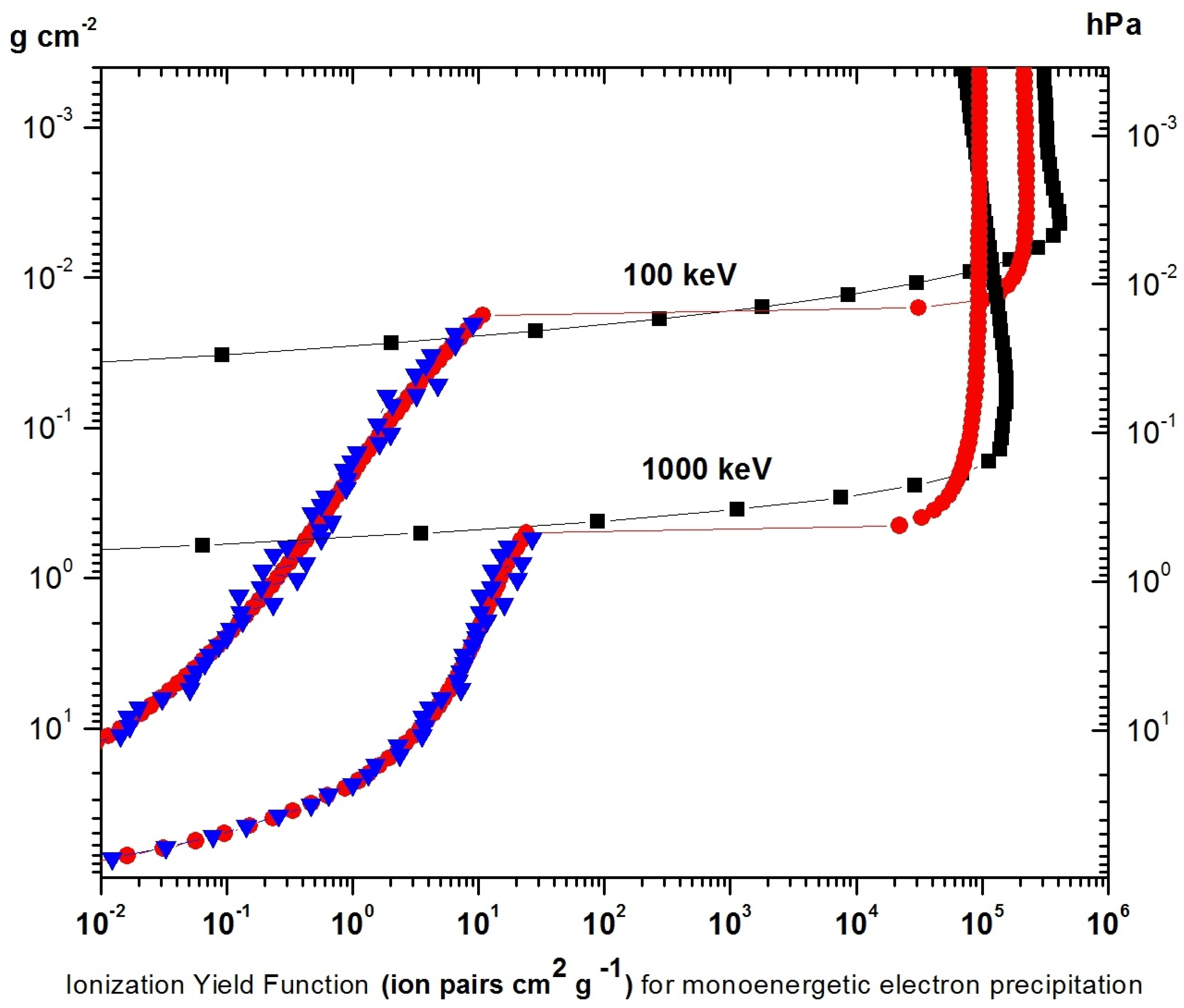
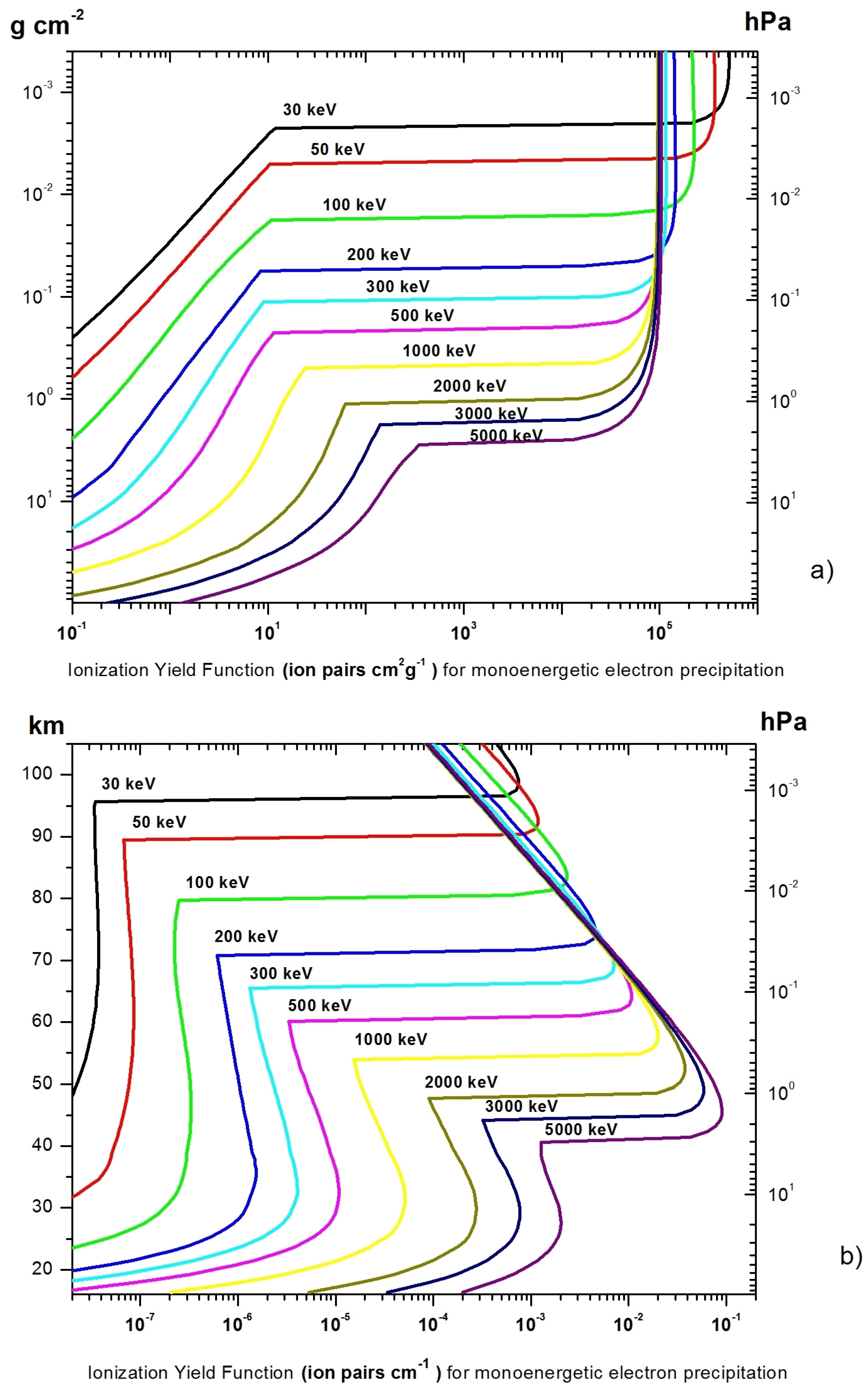
3. Atmospheric Ionization Yield Function for EEP with Isotropic Incidence

Here, we perform a calculation of the yield function Y ( x , E ) of monoenergetic electron beams with the energy of primary particles E in the atmospheric depth x (in g cm 2 ). Direct ionization by primary electrons is calculated analytically. Within this approach, we started our computations using the formalism presented in detail by [25]. Here, we assumed that electrons with initial kinetic energy E penetrate from the upper layer of the atmosphere (x = 0) from the zenith angle ϑ . The elastic scattering is neglected, and only the ionization process is considered.
The electron energy E after passing the thickness l (g cm 2 ) along the electron trajectory can be calculated as follows:
R ( E ) R ( E ) = l = x / cos ϑ
where R ( E ) is the path length of an electron with energy E due to ionization losses.
The differential ionization rate at the atmospheric depth x is defined as follows:
d q d x ( x , E ) = 1 cos ϑ · d q d l ( l , E ) = 1 35 e V · d E d l ( E ) · 1 cos ϑ
where E is defined from Equation (2). Note that d x = cos ϑ · d l and d E / d l ( E ) —the electron stopping power due to ionization losses. We assume that, on average, one ion–electron pair is produced per each 35 eV of deposited energy [26].
For the isotropic unit flux of precipitating electrons impinging on the top of the atmosphere from the solid angle Ω at d F / d Ω = c o s ϑ , the ionization yield function Y ( x , E ) is defined as
Y ( x , E ) = d q d x · d F d Ω d Ω = 2 π · 0 1 d q d l ( l , E ) d cos ϑ .
Figure 1 presents the calculated yield function (red lines with circles) for E: 100 keV and 1000 keV. For the comparison in Figure 1, the black lines with squares depict direct ionization yield functions for isotropic precipitating electrons according to Reference [20].
A sharp break in the yield function with an increase in thickness is due to the stopping power energy range of primary electron deposition. At lower altitudes (greater thicknesses), ionization is performed by the secondary Bremsstrahlung radiation. Ionization due to the Bremsstrahlung (blue triangles in Figure 1) was computed using the GEANT4 simulation tool PLANETOCOSMICS (http://cosray.unibe.ch/~laurent/planetocosmics/ accessed on 10 September 2021) with the NRLMSISE 00 atmospheric model [27]. The results of these calculations are approximated by the standard deviation function on a logarithmic scale (red curves with circles in Figure 1).
Figure 2 demonstrates EEP parameterization or ion production, where the ionization yield function with primary ionization induced via a direct electron impact and the secondary was mostly due to Bremsstrahlung radiation. The top panel, (a) of Figure 2 shows the ionization yield function Y ( x , E ) (ion pairs cm 2 g 1 ) vs. atmospheric depth x (g cm 2 ) due to the isotropic monoenergetic one-electron precipitation with an energy electron range of 30 keV–5000 keV. These ion productions or ionization yield function Y ( x , E ) (ion pairs cm 2 g 1 ) are presented as a look-up table in the Supplementary Materials of this paper.
The bottom panel, (b) of Figure 2 shows the dependence of the product Y ( x , E ) · ρ (ion pairs cm 1 ) on height (not thickness) in the atmosphere. ρ ( h ) is the atmospheric density at a height of h. Multiplying the yield function Y ( x , E ) (presented in the Supplementary Materials) by the real density of the atmosphere ρ ( h ) , one can calculate the ionization rates of the atmosphere at a given height of h.

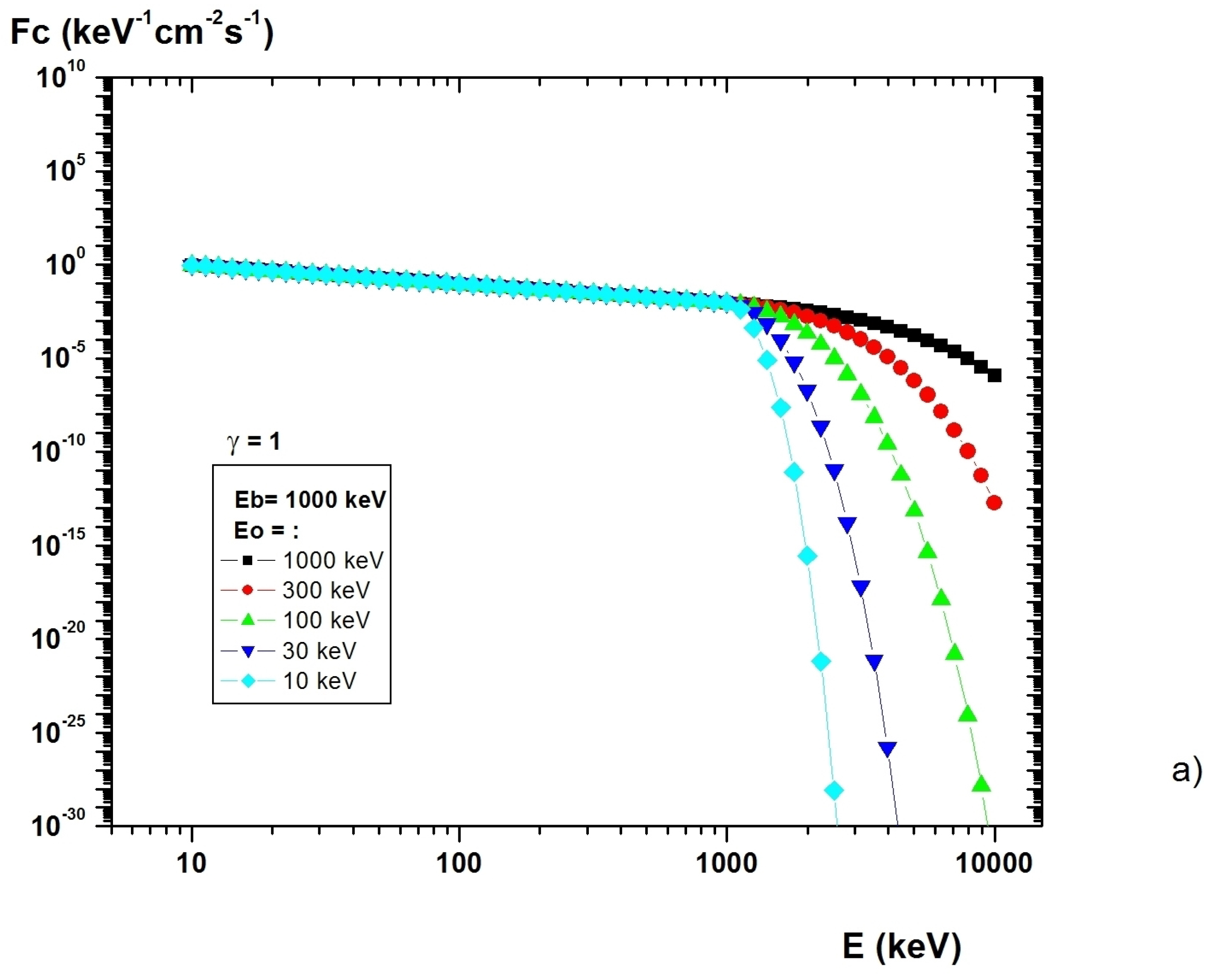
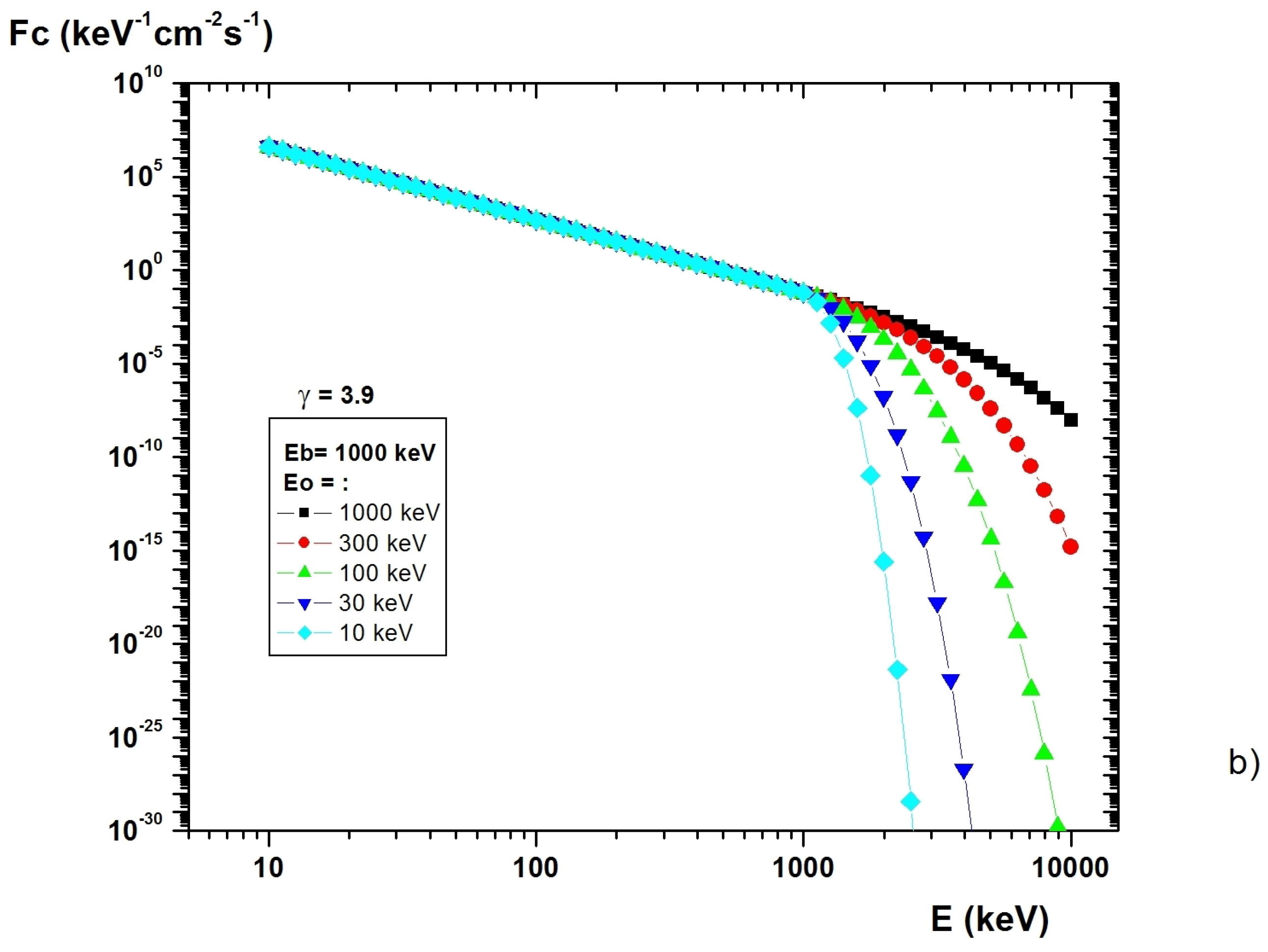
4. Spectra Function for Energetic Electron Precipitation

Retrieving ionization rates requires knowledge of the energy spectra and parameterization of ion production via ionization yield functions. The parametrization of ion production into atmosphere or yield function Y ( x , E ) was discussed previously in Section 3 and presented in Supplementary Material. The distribution of the energy spectra requires different fitting functions covering the same energy range, which makes the calculation of ionization rates ambiguous [28]. In this section, we consider various types of spectra distributions that allow us to fit the EEP fluxes and energy range as well as to propose a new combined spectral distribution F c ( E ) covering satellite and balloon observations in the EEP energy range.

4.1. Exponential Spectral Distribution

Generally, the exponential-law function of energy spectra is used for fitting balloon-borne [4] and rocket [29] observations. In this case, the form of the electron energy spectrum is fitted using a function of exponential law:
F e ( E ) = F o · exp E E o ,
where F e ( E ) is the differential flux of precipitating electrons with kinetic energy E, E o is the characteristic energy of precipitating electrons, and F o is a parameter of the flux of incident electrons (cm 2 s 1 keV 1 ). The characteristic energy of the electron spectra is from several keV to tens of MeV [4]. Such a type of electron spectra has also been used in many other studies fitting balloon-borne measurements, e.g., [3,30].

4.2. Maxwellian Spectral Distribution

The calculation of the ionization rates from the Maxwellian type of electron energy spectra F M ( E ) (cm 2 s 1 keV 1 ) can be expressed based on satellite and ground-based measurements [20,31,32,33]. The Maxwellian energy distribution is specified by
F M ( E ) = Q o 2 E o 3 E · exp E E o ,
where E o is characteristic energy (in keV), Q o is the total precipitating energy flux (keV cm 2 s 1 ). Auroral electrons of low energies (<30 keV) are in a quasi-equilibrium state, which is described by the Maxwellian energy distribution [34,35,36].

4.3. The Generalized Lorentzian (or κ -) Spectral Distribution

The source of precipitating electrons is the plasma sheet region of the magnetotail. The suprathermal populations of electrons are well described by the so-called Kappa κ or generalized Lorentzian distributions [37]. Due to these facts, one can suggest that the shape of electron energy distribution in the plasma sheet should be reflected in the energy distribution of precipitating electrons [33]. The κ distribution [20], which is Maxwellian at low energies and power-law at high energies, can be presented as follows:
F L ( E ) = Q o 2 E 0 3 · ( κ 1 ) ( κ 2 ) κ 2 · E 1 + E κ E o ( κ + 1 ) ,
where E o is characteristic energy and κ is the spectral gradient. F L ( E ) is the κ distribution of the differential energy spectrum. Q o is the total precipitating energy flux (keV cm 2 s 1 ).
Direct satellite-based spectral measurements can be approximated using one of these types of the spectral distribution. Reference [38] suggested that, for some cases, a fit by kappa distribution is more appropriate. We note that the κ distribution of differential energy spectrum (Equation (7)) becomes the Maxwellian distribution (Equation (6)) as κ [39]. The generalized Lorentzian distribution can be used with Maxwellian as additional high energy component of an energy spectrum of precipitating electrons [32].

4.4. Power-Law Spectral Distribution

Generally, the power-law function of spectra is used to fit satellite observations of solar protons and electrons [32,40,41,42,43] and medium energies (30 keV–1000 keV) electrons [44].
An example of a spectra, in power-law format is the one presented by [44]:
F p ( E ) = F o · E k ,
where F p ( E ) is the power-law integral energy spectrum, F o is a parameter of the flux of incident electrons (cm 2 s 1 keV 1 ), and k is the spectral gradient that can be calculated using a scheme described by [45]. It should be noted that the lower energy limit for this particular approximation was 30 keV and that the upper limit was 1 MeV [44].

4.5. Combined Spectral Distribution

Here, we propose a new form of combined spectral distribution that allows us to cover an energy range from tens of keV up to several MeV based on observation by satellite and balloon data.
F c ( E ) = F o · { E γ i f   E < E b , E γ ( E E b ) δ · exp ( E E b E o ) i f   E > E b .
Here, δ = E b E o , E b is a characteristic energy of electron’s spectrum and E o is the characteristic energy on a part of the spectrum of electrons where the spectrum decreases sharply. For an energy E = E b , parts of the function F c ( E ) and their first derivatives are stitched together. F o is a parameter of the flux of incident electrons (cm 2 s 1 keV 1 ). For E < E b , the power spectrum uses a spectral index γ . The function F c ( E ) is continuous at the respective energy along with its first derivative.
An example of such a type of combined spectral distribution F c ( E ) can be seen in Figure 3. In Figure 3, on the top and bottom panels, the energies band from 10 keV to 1000 keV that can be covered by satellites, as for example, by MEPED instrument of NOAA POES satellite, that usually are fitted by the power-law spectral distribution and balloon observations that usually are fitted by the exponential spectral distribution. E 0 = 1000 keV is characteristic energy on a part of the spectrum of electrons where spectrum decreases sharply; see Figure 3. Using proposed combined spectral distribution allows for describing balloon and satellite observations simultaneously.

5. Conclusions

In this paper, we presented a new parameterization of ion production and new spectra function for computation of ionization rates induced by energetic electron precipitation. A new parameterization of atmospheric ionization in the Earth’s atmosphere includes a yield function for isotropically precipitating monoenergetic (30 keV to 5 MeV) electrons and ionization via Bremsstrahlung radiation. We propose a favorable method for computation of the ionization rates forced by EEP using the new parameterization of ion production and a new spectrum shape, which allows one to take into account the range of precipitating particles from tens of keV to several MeV. A new function of spectra fit will also be helpful for obtaining information about EEP from satellite and balloon observations. A new look-up table with ion production/yield function for isotropically precipitating monoenergetic electrons can be easily used for computation of ionization rates and can further be used by atmospheric and chemistry-climate models for accurate quantification of atmospheric parameters during energetic electron precipitation.

Supplementary Materials

The following are available online at https://www.mdpi.com/article/10.3390/rs13204161/s1. The Supplementary Materials present a new look-up table of ionization yield functions inducing isotropically precipitating monoenergetic electrons (30 keV–5 MeV) and ionization via their Bremsstrahlung radiation; for an explanation, see Section 3. The new look-up table with ion production for isotropically precipitating monoenergetic electrons can be used for the scheme of ionization rates calculation described in Section 2.

Author Contributions

I.M., G.K., and A.A. discussed the idea and wrote the manuscript. G.K. and I.M. calculated and prepared the ionization yield functions. A.M. computed the ionization due to the Bremsstrahlung (blue triangles in Figure 1). G.K. proposed the combined spectral distribution. I.M. visualized this work. All authors have read and agreed to the published version of the manuscript.

Funding

I.M.’s work on the paper’s idea, yield functions, visualization and preparation of the paper was supported by a grant from the Russian Science Foundation (Project RSF 20-67-46016). The work of A.A. was supported by the Russian Foundation for Basic Research (Project RFBR 20-55-12020). The work on spectra preparation was conducted by I.M. in the SPBU “Ozone Layer and Upper Atmosphere Research Laboratory” supported by the Ministry of Science and Higher Education of the Russian Federation under agreement 075-15-2021-583. A.M. acknowledges support by the Academy of Finland (Project 330064 QUASARE).

Institutional Review Board Statement

Not applicable.

Informed Consent Statement

Not applicable.

Data Availability Statement

The look-up table of EEP ionization yield functions are presented in the Supplementary Material.

Conflicts of Interest

The authors declare no conflict of interest.

References

  1. Lam, M.M.; Horne, R.B.; Meredith, N.P.; Glauert, S.A.; Moat-Grin, T.; Green, J.C. Origin of energetic electron precipitation >30 keV into the atmosphere. J. Geophys. Res. 2010, 115, A00F08. [Google Scholar] [CrossRef]
  2. Rodger, C.J.; Clilverd, M.A.; Green, J.C.; Lam, M.M. Use of POES SEM-2 observations to examine radiation belt dynamics and energetic electron precipitation into the atmosphere. J. Geophys. Res. 2010, 115, A04202. [Google Scholar] [CrossRef] [Green Version]
  3. Millan, R.M.; Lin, R.P.; Smith, D.M.; McCarthy, M.P. Observation of relativistic electron precipitation during a rapid decrease of trapped relativistic electron flux. Geophys. Res. Lett. 2007, 34, L10101. [Google Scholar] [CrossRef]
  4. Makhmutov, V.; Bazilevskaya, G.; Stozhkov, Y.; Svirzhevskaya, A.; Svirzhevsky, N. Catalogue of electron precipitation events as observed in the long-duration cosmic ray balloon experiment. J. Atmos. Sol.-Terr. Phys. 2016, 149, 258–276. [Google Scholar] [CrossRef]
  5. Mironova, I.A.; Artamonov, A.A.; Bazilevskaya, G.A.; Rozanov, E.V.; Kovaltsov, G.A.; Makhmutov, V.S.; Mishev, A.L.; Karagodin, A.V. Ionization of the Polar Atmosphere by Energetic Electron Precipitation Retrieved From Balloon Measurements. Geophys. Res. Lett. 2019, 46, 990–996. [Google Scholar] [CrossRef] [Green Version]
  6. Mironova, I.A.; Bazilevskaya, G.A.; Kovaltsov, G.A.; Artamonov, A.A.; Rozanov, E.V.; Mishev, A.; Makhmutov, V.S.; Karagodin, A.V.; Golubenko, K.S. Spectra of high energy electron precipitation and atmospheric ionization rates retrieval from balloon measurements. Sci. Total Environ. 2019, 693, 133–242. [Google Scholar] [CrossRef] [PubMed]
  7. Lejeune, G.; Lathuillere, C.; Kofman, W. On the possibility to measure the high altitude light ion concentrations with EISCAT. Ann. Geophys. 1982, 38, 467–471. [Google Scholar]
  8. Sinnhuber, M.; Nieder, H.; Wieters, N. Energetic Particle Precipitation and the Chemistry of the Mesosphere/Lower Thermosphere. Surv. Geophys. 2012, 33, 1281–1334. [Google Scholar] [CrossRef]
  9. Mironova, I.; Aplin, K.; Arnold, F.; Bazilevskaya, G.; Harrison, R.; Krivolutsky, A.; Nicoll, K.; Rozanov, E.; Turunen, E.; Usoskin, I. Energetic Particle Influence on the Earth’s Atmosphere. Space Sci. Rev. 2015, 194, 1–96. [Google Scholar] [CrossRef] [Green Version]
  10. Rozanov, E.; Calisto, M.; Egorova, T.; Peter, T.; Schmutz, W. Influence of the Precipitating Energetic Particles on Atmospheric Chemistry and Climate. Surv. Geophys. 2012, 33, 483–501. [Google Scholar] [CrossRef] [Green Version]
  11. Arsenovic, P.; Rozanov, E.; Stenke, A.; Funke, B.; Wissing, J.; Mursula, K.; Tummon, F.; Peter, T. The influence of Middle Range Energy Electrons on atmospheric chemistry and regional climate. J. Atmos. Sol.-Terr. Phys. 2016, 149, 180–190. [Google Scholar] [CrossRef] [Green Version]
  12. Eyring, V.; Bony, S.; Meehl, G.A.; Senior, C.A.; Stevens, B.; Stouffer, R.J.; Taylor, K.E. Overview of the Coupled Model Intercomparison Project Phase 6 (CMIP6) experimental design and organization. Geosci. Model Dev. 2016, 9, 1937–1958. [Google Scholar] [CrossRef] [Green Version]
  13. Matthes, K.; Funke, B.; Andersson, M.E.; Barnard, L.; Beer, J.; Charbonneau, P.; Clilverd, M.A.; Dudok de Wit, T.; Haberreiter, M.; Hendry, A.; et al. Solar forcing for CMIP6 (v3.2). Geosci. Model Dev. 2017, 10, 2247–2302. [Google Scholar] [CrossRef] [Green Version]
  14. Rees, M. Auroral ionization and excitation by incident energetic electrons. Planet. Space Sci. 1963, 11, 1209–1218. [Google Scholar] [CrossRef]
  15. Lazarev, V.I. Absorption of the energy of an electron beam in the upper atmosphere. Geomagn. Aeron. 1967, 7, 219. [Google Scholar]
  16. Berger, M.J.; Seltzer, S.M. Bremsstrahlung in the atmosphere. J. Atmos. Sol.-Terr. Phys. 1972, 34, 85–108. [Google Scholar] [CrossRef]
  17. Roble, R.G.; Ridley, E.C. An auroral model for the NCAR thermospheric general circulation model (TGCM). Ann. Geophys. 1987, 5A, 369. [Google Scholar]
  18. Sergienko, T.E.; Ivanov, V.E. A new approach to calculate the excitation of atmospheric gases by auroral electron impact. Ann. Geophys. 1993, 11, 717–727. [Google Scholar]
  19. Fang, X.; Randall, C.E.; Lummerzheim, D.; Solomon, S.C.; Mills, M.J.; Marsh, D.R.; Jackman, C.H.; Wang, W.; Lu, G. Electron impact ionization: A new parameterization for 100 eV to 1 MeV electrons. J. Geophys. Res. 2008, 113, A09311. [Google Scholar] [CrossRef]
  20. Fang, X.; Randall, C.E.; Lummerzheim, D.; Wang, W.; Lu, G.; Solomon, S.C.; Frahm, R.A. Parameterization of monoenergetic electron impact ionization. Geophys. Res. Lett. 2010, 37, L22106. [Google Scholar] [CrossRef]
  21. Artamonov, A.A.; Mishev, A.L.; Usoskin, I.G. Model CRAC:EPII for atmospheric ionization due to precipitating electrons: Yield function and applications. J. Geophys. Res. (Space Phys.) 2016, 121, 1736–1743. [Google Scholar] [CrossRef] [Green Version]
  22. Artamonov, A.; Mironova, I.; Kovaltsov, G.; Mishev, A.; Plotnikov, E.; Konstantinova, N. Calculation of atmospheric ionization induced by relativistic electrons with non-vertical precipitation: Update of model CRAC:EPII. Adv. Space Res. 2017, 59, 2295–2300. [Google Scholar] [CrossRef] [Green Version]
  23. Xu, W.; Marshall, R.A.; Tyssøy, H.N.; Fang, X. A generalized method for calculating atmospheric ionization by energetic electron precipitation. J. Geophys. Res. (Space Phys.) 2020, 125, e2020JA028482. [Google Scholar] [CrossRef]
  24. Xu, W.; Marshall, R.A.; Tobiska, W.K. A Method for Calculating Atmospheric Radiation Produced by Relativistic Electron Precipitation. Space Weather 2021. [Google Scholar] [CrossRef]
  25. Usoskin, I.G.; Kovaltsov, G.A.; Mironova, I.A. Cosmic ray induced ionization model CRAC:CRII: An extension to the upper atmosphere. J. Geophys. Res. 2010, 115, D10302. [Google Scholar] [CrossRef] [Green Version]
  26. Porter, H.S.; Jackman, C.H.; Green, A.E.S. Efficiencies for production of atomic nitrogen and oxygen by relativistic proton impact in air. J. Chem. Phys. 1976, 65, 154–167. [Google Scholar] [CrossRef]
  27. Picone, J.M.; Hedin, A.E.; Drob, D.P.; Aikin, A.C. NRLMSISE-00 empirical model of the atmosphere: Statistical comparisons and scientific issues. J. Geophys. Res. (Space Phys.) 2002, 107, 1468. [Google Scholar] [CrossRef]
  28. Mironova, I.; Sinnhuber, M.; Rozanov, E. Energetic electron precipitation and their atmospheric effect. E3S Web Conf. 2020, 196. [Google Scholar] [CrossRef]
  29. Goldberg, R.A.; Jackman, C.H.; Barcus, J.R.; Soraas, F. Nighttime auroral energy deposition in the middle atmosphere. J. Geophys. Res. 1984, 89, 5581–5596. [Google Scholar] [CrossRef] [Green Version]
  30. Comess, M.D.; Smith, D.M.; Selesnick, R.S.; Millan, R.M.; Sample, J.G. Duskside relativistic electron precipitation as measured by SAMPEX: A statistical survey. J. Geophys. Res. (Space Phys.) 2013, 118, 5050–5058. [Google Scholar] [CrossRef]
  31. Lummerzheim, D.; Rees, M.H.; Romick, G.J. The application of spectroscopic studies of the aurora to thermospheric neutral composition. Planet. Space Sci. 1990, 38, 67–78. [Google Scholar] [CrossRef]
  32. Codrescu, M.V.; Fuller-Rowell, T.J.; Roble, R.G.; Evans, D.S. Medium energy particle precipitation influences on the mesosphere and lower thermosphere. J. Geophys. Res. 1997, 102, 19977–19988. [Google Scholar] [CrossRef]
  33. Mori, H.; Ishii, M.; Murayama, Y.; Kubota, M.; Sakanoi, K.; Yamamoto, M.; Monzen, Y.; Lummerzheim, D.; Watkins, B. Energy distribution of precipitating electrons estimated from optical and cosmic noise absorption measurements. Ann. Geophys. 2004, 22, 1613–1622. [Google Scholar] [CrossRef] [Green Version]
  34. Robinson, R.; Vondrak, R.; Miller, K.; Dabbs, T.; Hardy, D. On calculating ionospheric conductances from the flux and energy of precipitating electrons. J. Geophys. Res. 1987, 92, 2565–2570. [Google Scholar] [CrossRef]
  35. Frahm, R.; Winningham, J.; Sharber, J.; Link, R.; Crowley, G.; Gaines, E.; Chenette, D.; Anderson, B.; Potemra, T. The diffuse aurora: A significant source of ionization in the middle atmosphere. J. Geophys. Res. 1997, 102, 28203–28214. [Google Scholar] [CrossRef]
  36. Solomon, S.C. Auroral particle transport using Monte Carlo and hybrid methods. J. Geophys. Res. 2001, 106, 107–116. [Google Scholar] [CrossRef] [Green Version]
  37. Pierrard, V.; Lazar, M. Kappa distributions: Theory and applications in space plasmas. Sol. Phys. 2010, 267, 153–174. [Google Scholar] [CrossRef] [Green Version]
  38. Sharber, J.R.; Frahm, R.A.; Link, R.; Crowley, G.; Winningham, J.D.; Gaines, E.E.; Nightingale, R.W.; Chenette, D.L.; Anderson, B.J.; Gurgiolo, C.A. UARS particle environment monitor observations during the November 1993 storm: Auroral morphology, spectral characterization, and energy deposition. J. Geophys. Res. 1998, 103, 26307–26322. [Google Scholar] [CrossRef]
  39. Vasyliunas, V.M. A survey of low-energy electrons in the evening sector of the magnetosphere with OGO 1 and OGO 3. J. Geophys. Res. 1968, 73, 2839–2884. [Google Scholar] [CrossRef]
  40. Vampola, A.L.; Gorney, D.J. Electron energy deposition in the middle atmosphere. J. Geophys. Res. 1983, 88, 6267–6274. [Google Scholar] [CrossRef]
  41. Schroter, J.; Heber, B.; Steinhilber, F.; Kallenrode, M.B. Energetic particles in the atmosphere: A Monte-carlo simulation. Adv. Space Res. 2006, 37, 1597–1601. [Google Scholar] [CrossRef]
  42. Wissing, J.; Kallenrode, M.-B. Atmospheric ionization module Osnabrück (AIMOS): A 3-D model to determine atmospheric ionization by energetic charged particles from different populations. J. Geophys. Res. 2009, 114, A06104. [Google Scholar] [CrossRef] [Green Version]
  43. Clilverd, M.A.; Rodger, C.J.; Gamble, R.J.; Ulich, T.; Raita, T.; Seppälxax, A.; Green, J.C.; Thomson, N.R.; Sauvaud, J.-A.; Parrot, M. Ground-based estimates of outer radiation belt energetic electron precipitation fluxes into the atmosphere. J. Geophys. Res. (Space Phys.) 2010, 115, A12304. [Google Scholar] [CrossRef] [Green Version]
  44. van de Kamp, M.; Seppälxax, A.; Clilverd, M.A.; Rodger, C.J.; Verronen, P.T.; Whittaker, I.C. A model providing long-term data sets of energetic electron precipitation during geomagnetic storms. J. Geophys. Res. (Atmos.) 2016, 121, 12520–12540. [Google Scholar] [CrossRef] [Green Version]
  45. Birch, M.J.; Hargreaves, J.; Bromage, B.J.I.; Evans, D. Effects of high-speed solar wind on energetic electron activity in the auroral regions during July 1–2, 2005. J. Atmos. Sol.-Terr. Phys. 2009, 71, 1190–1209. [Google Scholar] [CrossRef]
Figure 1. The yield function for isotropic monoenergetic precipitating electrons with energies 100 keV and 1000 keV. Blue triangles are ionization due to the Bremsstrahlung radiation computed by using the GEANT4. Red curves with circles are ionization presented in a look-up table in the Supplementary Materials. Black lines with squares—direct ionization yield functions were taken from Reference [20].
Remotesensing 13 04161 g001
Figure 2. Ion production or yield function induced by the isotropic monoenergetic electron precipitation with an electron energy range of 30 keV–5000 keV. Top panel, (a): yield function Y ( x , E ) (ion pairs cm 2 g 1 ) vs. atmospheric depth x (g cm 2 ); see also the Supplementary Materials of this paper. Bottom panel, (b): product Y ( x , E ) · ρ (ion pairs cm 1 ) vs. atmospheric altitude h (km).
Remotesensing 13 04161 g002
Figure 3. Energetic electron precipitation with an energy range from tens keV to several MeV fitted by combined spectral distribution F c ( E ) . Top panel, (a): combined spectral distribution F c ( E ) with a spectral index γ = 1 . Bottom panel, (b): combined spectral distribution F c ( E ) with a spectral index γ = 3.9 . The top panel (a) and bottom panel (b) have the same E o and E b , and the only difference is in a spectral index γ .
Remotesensing 13 04161 g003aRemotesensing 13 04161 g003b
Publisher’s Note: MDPI stays neutral with regard to jurisdictional claims in published maps and institutional affiliations.

