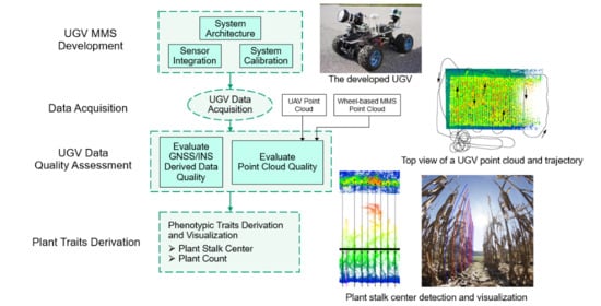
Article

Development of a Miniaturized Mobile Mapping System for In-Row, Under-Canopy Phenotyping

Lyles School of Civil Engineering, Purdue University, West Lafayette, IN 47907, USA
*
Author to whom correspondence should be addressed.
These authors contributed equally to this work.
Remote Sens. 2021, 13(2), 276; https://doi.org/10.3390/rs13020276
Submission received: 17 December 2020 / Revised: 10 January 2021 / Accepted: 11 January 2021 / Published: 14 January 2021

Abstract

:
This paper focuses on the development of a miniaturized mobile mapping platform with advantages over current agricultural phenotyping systems in terms of acquiring data that facilitate under-canopy plant trait extraction. The system is based on an unmanned ground vehicle (UGV) for in-row, under-canopy data acquisition to deliver accurately georeferenced 2D and 3D products. The paper addresses three main aspects pertaining to the UGV development: (a) architecture of the UGV mobile mapping system (MMS), (b) quality assessment of acquired data in terms of georeferencing information as well as derived 3D point cloud, and (c) ability to derive phenotypic plant traits using data acquired by the UGV MMS. The experimental results from this study demonstrate the ability of the UGV MMS to acquire dense and accurate data over agricultural fields that would facilitate highly accurate plant phenotyping (better than above-canopy platforms such as unmanned aerial systems and high-clearance tractors). Plant centers and plant count with an accuracy in the 90% range have been achieved.

Graphical Abstract

1. Introduction

The ever-increasing human population stipulates for a sustained supply of staple crops. Compared to 2005, it is forecast that the global crop demand will increase at least 100% by 2050 [1]. To meet this demand with minimal environmental impacts, the attainment of high yields from existing croplands is of great importance. Genetic improvement of staples has accounted for more than half of the past increase in yield [2]. The objective of genetic breeding programs is producing genotypes that can succeed existing cultivars on the market to increase crop resistance to pests and diseases, reduce the requirement for water and nutrient uptake, and increase nutritional value and grain yield. The main challenge for a genetic breeding program is correlating seed genotype and plant phenotypic traits under field conditions [3]. More specifically, high-throughput phenotyping under field conditions is the bottleneck influencing the success of any genetic breeding program.
Recent advances in near-surface remote sensing technologies are playing a crucial role in advancing the domain of high-throughput phenotyping [4,5,6]. Airborne systems (unmanned aerial vehicles and manned aircrafts), wheel-based mapping platforms, and ground-based static sensors are gaining wide recognition as efficient tools to non-destructively capture plant traits [7,8,9,10,11]. Despite the increased geometric, spectral, and temporal resolution of modern remote sensing platforms, they still struggle in providing key phenotypic traits, such as stalk diameter, leaf angles, ear heights, silking stages, and leaf area index (LAI), with high accuracy. This lack is mainly attributed to the following limitations:
(a)
Temporal/spatial resolution: Unmanned aerial vehicles (UAVs) facilitate high temporal resolution since they can be flown multiple times throughout the growing season. However, the spatial resolution, especially for light detection and ranging (LiDAR) data, is low due to the flying height. On the contrary, close-range, wheel-based phenotyping tractors provide high spatial resolution but their temporal resolution relies heavily on the weather conditions since they cannot be driven, for instance, until several days following rain because of potential soil compaction.
(b)
Platform mobility: Static terrestrial laser scanners (TLSs) can obtain high-density point clouds, but the density drops quickly as the distance from the sensor increases. The acquisition of data that adequately captures the entire field requires a setup of multiple TLS stations. Furthermore, derived point clouds from different stations need to be registered to align them to a common reference frame. However, the absence of uniquely identifiable features in the individual scans makes the registration process challenging. A potential solution to this problem is deploying artificial targets. However, those targets are limited in terms of coverage and spatial distribution, not to mention the practical challenge in the scalability of such a data acquisition strategy.
(c)
Terrain navigation: UAVs are not affected by the terrain topography, whereas wheel-based tractors cannot operate efficiently in rough terrain since they need to traverse along the rows while being mindful of the interference with the crops. Moreover, large and heavy wheel-based tractors will introduce soil compaction issues.
(d)
Under-canopy scanning: Most UAVs and wheel-based platforms cannot acquire reliable under-canopy data. LiDAR sensors onboard these platforms can penetrate the canopy to some extent but in the later crop growth stages, penetration would be further limited in capturing under-canopy characteristics, such as ear height and stalk diameter. RGB imagery, on the other hand, suffers from occlusions by the canopy.
These limitations necessitate the development of a small, lightweight platform that would ensure high temporal and spatial resolution and is easily deployable and maneuverable within any agricultural field at varying growth stages, without introducing soil compaction. Therefore, the focus of this paper is the development and evaluation of a new unmanned ground vehicle (UGV) mobile mapping system (MMS) that overcomes the shortcomings of UAVs, large wheel-based mobile platforms, and static TLSs. This problem is dealt with in three stages, as illustrated by the flowchart in Figure 1.
(a)
UGV MMS Development: First, the research addresses the platform architecture design, sensor integration, and system calibration. The system architecture design encompasses the choice of sensors as well as their configuration to maximize the details captured by the sensors.
(b)
UGV Data Quality Assessment: Once the sensor suite has been integrated and calibrated, the next step of this research is to conduct a comprehensive quality assessment of the processed data, i.e., global navigation satellite system/inertial navigation system (GNSS/INS) trajectory and derived point clouds from the LiDAR sensor. The UGV trajectory is evaluated to understand the impact of the plant canopy on the acquired data by the GNSS/INS unit. To the best of the authors’ knowledge, there is no commercially available UGV system with comparable system specifications and integration strategy that allow the derivation of centimeter-level accuracy point clouds. Therefore, the quality of the UGV point cloud is analyzed by comparing its level of detail and alignment with point clouds from UAV and large wheel-based mobile mapping systems, whose absolute accuracy has been evaluated in prior research [12,13].
(c)
Plant Trait Derivation: The last stage of this research is to demonstrate the potential of high-resolution, under-canopy data for deriving plant traits beyond plant height, such as plant location and plant count. These traits are then visualized in 2D imagery as well as 3D point clouds.
The paper starts by providing an overview of prior related research in Section 2. Next, Section 3 covers the first challenge, namely UGV MMS development. Section 4 then provides details about the field over which the UGV, along with other systems—UAV and wheel-based MMSs—are used to acquire experimental datasets for this research. It also includes details about the various MMSs as well as the data acquisition missions. In Section 5, the approaches adopted for quality assessment of the derived trajectory and point cloud from GNSS/INS and LiDAR units, respectively, are introduced along with experimental results to validate the claims of this research. Section 6 demonstrates the potential of acquired under-canopy data for deriving plant traits. Finally, Section 7 discusses the conclusions drawn from this research along with future research directions in the domain of UGV-based agricultural phenotyping.

2. Related Work

This section discusses prior work related to the domains of remote sensing techniques and advancements in the development of unmanned ground vehicles for mapping in various agricultural environments. Ongoing research in the field of agricultural mapping has explored several remote sensing platforms for data acquisition, including static TLSs, wheel-based mobile mapping platforms, and unmanned aerial vehicles. Malambo et al. [14] used a TLS—Faro Focus X330—to acquire data over a sorghum field to estimate the counts and individual dimensions of sorghum panicles (panicle length, width, and height). They developed a density-based clustering strategy to derive the desired information and validated the approach through experimental results that indicated an overall accuracy of 89.3% for panicle detection (or counting) with 10.7% omission and 14.3% commission rates. However, they observed that TLS data are prone to occlusion by foliage, thus resulting in the omission of some panicles. Su et al. [15] used a TLS to evaluate the performance of LiDAR in monitoring time series maize phenotypes in field practices and analyzed the growth dynamics of different maize varieties under drought stress. The results showed that terrestrial LiDAR data could estimate plant height, plant area index, and project leaf area with an accuracy of 96%, 70%, and 92%, respectively. Again, occlusions caused by objects within the field of view affected the final accuracy of the results.
A significant amount of research has also been conducted on the use of above-canopy, ground-based MMSs for agricultural phenotyping applications. Milioto et al. [16] used RGB imagery from a ground-based MMS for the real-time semantic segmentation of crops and weeds with the help of a convolutional neural network (CNN) framework. The ground-based MMS used in their study was the “Bosch Deepfield Robotics BoniRob UGV”, which is a robotic high-clearance tractor intended for precision agriculture. Pérez-Ruiz et al. [17] developed and evaluated a ground-based MMS for high-throughput phenotyping in wheat breeding trials. They used 2D LiDAR, RGB imagery, and multispectral imagery to derive traits such as plant height, normalized differential vegetation index (NDVI), and photochemical reflectance index (PRI). Qiu et al. [18] conducted high-throughput phenotyping, including the extraction of plant height and row spacing, using a wheel-based system equipped with a 3D LiDAR unit. Jiang et al. [19] developed a ground-based MMS for the multi-modal imaging of cotton fields. The system included an RGB-D camera, a thermal camera, and a hyperspectral camera, along with an onboard GNSS/INS unit. Ravi et al. [12] used a ground-based high-clearance tractor equipped with LiDAR and imaging systems for the high-throughput phenotyping of sorghum fields to extract plant height and canopy cover for early-stage biomass prediction.
UAVs are yet another type of remote sensing platform that are used for agricultural applications. Malambo et al. [20] conducted a study using UAV-based imagery for automated panicle counting in sorghum fields based on a deep learning framework for semantic segmentation. Their study indicated an overall detection accuracy of 94%. Ravi et al. [21] introduced a multi-sensor UAV platform consisting of an RGB camera, a hyperspectral camera, a LiDAR unit, and a GNSS/INS position and orientation system for data acquisition over agricultural fields. The platform was used for plant height and canopy cover estimation for sorghum fields. Zhou et al. [22] used UAV-based LiDAR data to analyze plant height changes within lodged maize crops. Xu et al. [23] investigated the use of multispectral imagery captured by a UAV platform for cotton plant phenotyping.
While above-canopy remote sensing platforms—ground-based and UAV-based platforms—have been explored significantly for agricultural applications, the use of under-canopy remote sensing platforms is a budding research domain. Exploring under-canopy mapping entails the development of platforms with a choice of suitable onboard sensors, the configuration of such sensors, and, lastly, comparison of these platforms relative to existing above-canopy platforms. The development of novel mapping platforms along with the associated challenges have been presented by Velas et al. [24] and Cong et al. [25] for backpack and UGV scanning systems, respectively. Besides the integration of sensors on mapping platforms, the acquired data (such as LiDAR, RGB cameras, GNSS, and INS) have to be synchronized properly, followed by conducting an accurate calibration to ensure the accuracy of the derived products. Among these challenges, Velas et al. [24] addressed the problem of accurate trajectory estimation by developing an algorithm for odometry estimation using dual LiDAR units onboard a backpack system. Cong et al. [25] addressed the trajectory estimation using LiDAR-based simultaneous localization and mapping (SLAM) for a UGV platform to map environments with moving targets. Pierzchała et al. [26] introduced a UGV platform for mapping forests with the help of LiDAR along with graph-SLAM to map tree positions and diameters.
Advancing the domain of UGV-based agricultural mapping is the basis for the presented research in this paper. More specifically, the presented research focuses on the developmental aspects of a UGV platform for in-field high-throughput phenotyping. The paper also presents a detailed comparison with existing platforms in terms of the resultant quality of derived products and its potential towards extracting plant centers and plant count automatically and efficiently.

3. Platform Architecture, Sensor Integration, and System Calibration

The UGV in this study was developed as an agricultural platform for in-row, under-canopy crop monitoring. Emphasis was placed on building a compact design to conveniently traverse in the narrow, mostly under a meter wide, row-to-row separation. At the same time, to obtain semantic and positional information of various plant features, an RGB camera and a 3D LiDAR sensor were used. The imagery data are also used to analyze the environment when there are any GNSS signal reception issues. In this regard, a large field of view RGB camera and a high measurement rate LiDAR sensor serve the purpose of proximal object scanning very well. The developed platform (Figure 2) consists of a base rover carrying a Sony α 7R RGB camera, a Velodyne VLP-16 Hi-Res 3D LiDAR sensor, and a Novatel SPAN-IGM GNSS/INS unit. The RGB camera, LiDAR, and GNSS/INS unit are rigidly fixed relative to one another. The rover is an all-terrain four-wheeled race car, which can be remotely controlled. The entire UGV has dimensions of about 0.6 m (length) × 0.4 m (width). Knowing that most commercial and research fields have a row-to-row separation of about 0.762 m (30 inches), one can argue that the UGV size, together with its ruggedness, allows the platform to be easily maneuvered between rows during data collection.
The SPAN-IGM unit provides direct georeferencing information, i.e., the position and orientation of the inertial measurement unit (IMU) body frame, at a rate of 125 Hz. After GNSS/INS data post-processing, the expected positional accuracy is ±2 cm and the accuracy for pitch/roll and heading is ±0.006° and ±0.019°, respectively [27]. These accuracy values, however, change depending on whether there has been a complete or partial outage of the GNSS signal reception due to an obstruction by the canopy. Table 1 shows the manufacturer-specified position and attitude accuracy of the SPAN-IGM in case of GNSS signal outage for certain durations.
The Velodyne VLP-16 Hi-Res consists of 16 radially oriented laser rangefinders with a 360° horizontal field of view and a 20° vertical field of view (±10° from the optical center line). This sensor can generate 300,000 points per second with a maximum range of 100 m at an accuracy of ±3 cm [28]. The LiDAR unit is mounted on the back of the platform with an upward tilt of about 30° from the horizontal plane. This directs the scan window to survey the ground as well as plants on both sides of the platform. Moreover, the tilt prevents any radio frequency (RF) interference with the GNSS antenna. The Sony α 7R camera is a 36.4 MP full-frame camera with a 7360 × 4912 complementary metal–oxide–semiconductor (CMOS) sensor array [29]. It uses a super-wide field of view fisheye lens with an 8 mm nominal focal length that captures highly detailed images of the surroundings, effectively eliminating the need for multiple cameras to capture imagery on both sides of the UGV. The camera is mounted at the front of the platform facing forward at an inclination of about 20° relative to the horizontal plane to keep the fisheye lens clear of any obstruction. It is synchronized to capture RGB imagery at a rate of one frame every 1.5 second. The computer used to activate the sensors and log the collected data is a single-board Raspberry Pi 4 module. Its low-cost user-interactive interface provides the ability to modify data-logging parameters and verify acquired data in the field.
The system integration architecture is summarized in Figure 3. The Velodyne VLP-16 LiDAR conforms to the industry standard protocol for time-tagging its observed points. It accepts two types of signal sent from the GNSS/INS unit—a pulse per second (PPS) and a time-stamp message such as the GPS satellite recommended minimum navigation sentence C (GPRMC) [28,30]. The PPS is short, under 20 microsecond (μs) wide pulse that synchronizes the second mark of the LiDAR internal clock with that of the GNSS receiver. Concurrently, the GPRMC message assigns a precise timestamp to the measured LiDAR points. The PPS and the GPRMC signals are usually sent through different wiring channels since they have different polarities. The shutter of the RGB camera is programmatically triggered through the onboard computer. However, due to a delay in the actual shutter action from the trigger time, the latter is not considered as the exposure time. Instead, the camera hotshoe-based time-tagging proposed by Elbahnasawy et al. [10] is employed, where the feedback from the hotshoe is sent to the GNSS/INS unit to mark the time of shutter action. This approach simplifies the data acquisition flow since all the time-related information is handled by the precise GNSS/INS clock, thus minimizing any time offset between the exposure and marked event.
Having rigidly mounted and integrated the sensors onboard the platform, the next step is to conduct a system calibration to estimate the intrinsic sensor parameters as well as the relative mounting parameters among the sensors. The coordinate systems for the GNSS/INS, camera, and LiDAR units are shown in Figure 4. The system calibration is crucial to ensure the accuracy of the resultant georeferenced information from the LiDAR and RGB camera. The camera calibration process estimates the interior orientation parameters (IOPs), which comprise principal point coordinates, principal distance, and lens distortions. The IOP estimates are derived using the proposed procedure by Choi et al. [31] for cameras with a fisheye lens. Then, the mounting parameters—lever arm and boresight angles—relating the onboard GNSS/INS to the RGB camera and LiDAR unit are estimated using the in situ calibration strategy proposed by Ravi et al. [32]. The system calibration estimates the mounting parameters by minimizing discrepancies among conjugate points, planes, and linear features extracted from LiDAR point clouds and images from different tracks. The joint calibration results in a properly aligned image and LiDAR data. For the LiDAR unit, the standard deviation of the estimated lever arm components along both the X and Y directions is ±1.1 cm, and those of the boresight angles are ±0.059°, ±0.027°, and ±0.025° for roll, pitch, and heading, respectively. The lever arm component along the Z direction was manually measured and fixed during the calibration as it would not cause any discrepancy between corresponding features in different tracks [33]. The accuracy of the final ground coordinates evaluated using the LiDAR error propagation calculator developed by Habib et al. [34] is in the range of ±1.5–2 cm at a sensor-to-object distance of 1 m. In the case of the RGB camera, the standard deviations of the estimated lever arm components along the X, Y, and Z directions are ±5.5 cm, ±5 cm, and ±5 cm, respectively, and those of the boresight angles are all ±0.1° for roll, pitch, and heading.
Once the mounting parameters are estimated, the reconstructed point cloud and RGB images are directly georeferenced to a common reference frame. Thus, the data from the two sensor modalities can be forward and backward projected using the estimated parameters. This projection will map a particular point from the LiDAR point cloud to images where the corresponding point is visible. Similarly, a point visible in two or more images can be used to derive the corresponding 3D coordinates. As an advantage, features that are unidentifiable in the point cloud or imagery can be looked up in the other modality. Figure 5 illustrates an example of the projection where the red dot in a LiDAR point cloud is projected onto the corresponding image, shown as a magenta-colored circle. In this figure, both the original image and its corresponding rectified image are shown. The rectified image is derived through conversion of the fisheye projection to a perspective projection using an effective focal length of 4 mm.

4. Dataset Acquisition and Description

Several outdoor data collection experiments were conducted to: (a) assess the quality of the derived trajectory from the GNSS/INS unit and point cloud from the LiDAR sensor onboard the UGV and (b) investigate the potential of deriving phenotypic attributes, such as plant centers and plant count, from the UGV point cloud. Datasets for this purpose were acquired over two maize fields at Purdue’s Agronomy Center for Research and Education (ACRE). The two fields are denoted as ACRE-9D and ACRE-12 hereafter. Figure 6 displays UAV-based orthophotos of the two fields. Field ACRE-9D consisted of 25 rows with 19 alleys, with an approximate row spacing of 0.762 m (30 inches). The planting orientation was approximately along the east–west direction. Field ACRE-12 had 44 rows with no alleys, and the row spacing was also 0.762 m. The planting orientation was approximately along the north–south direction.
While both LiDAR point cloud and camera images are affected by georeferencing problems, the focus of the subsequent discussion is evaluating the quality of the LiDAR point cloud since the manifestation of georeferencing artifacts within LiDAR data is more pronounced than for imagery. The quality assessment of the LiDAR point cloud is carried out through a comparison with point clouds obtained from other well-established, above-canopy phenotyping platforms, including UAV-based and wheel-based systems. The UAV-based system (shown in Figure 7a) consists of a Velodyne VLP-32C LiDAR unit, a Sony α 7R III RGB camera, and a Trimble APX-15 UAV v3 integrated GNSS/INS unit for direct georeferencing. The range accuracy of the VLP-32C is ±3 cm, with a maximum measurement range of 200 m [35]. For the APX-15 unit, the post-processing positional accuracy is ±2–5 cm and the accuracy for the roll/pitch and heading is ±0.025° and ±0.08°, respectively [36]. The expected accuracy of the derived point cloud is estimated using the LiDAR error propagation calculator developed by Habib et al. [34]. At a flying height of 50 m, the calculator suggests that the horizontal and vertical accuracy values are in the ±5–6 cm range at the nadir position. At the edge of the swath, the horizontal accuracy would be about ±8–9 cm and the vertical accuracy would be ±5–6 cm. The wheel-based high-clearance tractor MMS (shown in Figure 7b), hereafter denoted as “PhenoRover”, carries a Velodyne VLP-16 Hi-Res laser scanner, a Velodyne HDL-32E laser scanner, two FLIR Grasshopper3 RGB cameras, a Headwall Machine Vision push-broom hyperspectral scanner, and an Applanix POSLV 125 GNSS/INS unit for direct georeferencing. The range accuracy of the VLP-16 Hi-Res and HDL-32E is ±3 cm and ±2 cm, respectively [28,37]. For the POSLV 125, the post-processing positional accuracy is ±2–5 cm, and the attitude accuracy is ±0.025° and ±0.08° for the roll/pitch and heading, respectively [38]. The horizontal and vertical accuracy according to the LiDAR error propagation calculator developed by Habib et al. [34] is in the ±2–5 cm range, at a sensor-to-object distance of 5 m.
A total of five datasets were collected over the two maize fields. Datasets A-1 and A-2 were collected in ACRE-9D; and datasets B-1, B-2, and B-3 were acquired in ACRE-12. The data acquisition missions in ACRE-9D consisted of 4 ground tracks for the UGV and 3 aerial tracks for the UAV, both in the east–west direction. The number of tracks for the UGV, PhenoRover, and UAV over ACRE-12 were 8, 10, and 4, respectively. Table 2 lists the flight/drive-run configuration for each dataset. The small size of the UGV allowed it to traverse rows under the plant canopy with sufficient clearance on the sides. The drive-run configuration for the UGV was designed to have different track-to-track lateral distances to study its impact on the point density. Figure 8 shows the UGV making its way under the canopy along the rows of maize plants. Sample RGB images captured by the onboard camera during data acquisition in ACRE-9D and ACRE-12 are shown in Figure 9a,b, respectively. The two datasets were collected almost a month apart in the late season. The canopy cover was moderate to low depending on the growth stage at the time of data acquisition—the A-1 dataset has greener plants, whereas those in B-1 are senesced.
Figure 10 and Figure 11 present the reconstructed point cloud (colored by height from blue to red) and corresponding trajectory of the mobile mapping system (shown in black) for datasets collected at ACRE-9D and ACRE-12, respectively. The varying track-to-track lateral distances for the UGV can be observed in Figure 10a and Figure 11a. The point clouds collected by different systems are georeferenced to the Universal Transverse Mercator (UTM) coordinate system with NAD83 as the datum using the GNSS/INS trajectory information. One can observe that both ground-based systems were driven along the row to achieve non-destructive data acquisition. For the UAV, however, there is no such limitation on the flight line configuration. The UAV tracks depicted in Figure 10b and Figure 11c indicate that the former has tracks parallel to the rows, whereas the latter has tracks perpendicular to the rows.

5. Quality Assessment of Derived Trajectory and Point Clouds

This section investigates the quality of information derived from the UGV sensors. First, the quality of the GNSS/INS post-processed trajectory is assessed. Then, while considering the challenges with georeferencing, the relative accuracy of the derived point cloud is evaluated by comparing its level of detail as well as its horizontal and vertical alignment with point clouds from other platforms.

5.1. Impact of Canopy on GNSS/INS-Derived Trajectory

Given that the UGV in this study is designed for under-canopy mapping, there is a high probability of interruptions in the satellite signal received by the GNSS antenna while driving within the crop rows. Hence, a comprehensive review of the post-processed GNSS/INS trajectory is essential to identify factors that may affect its positional accuracy. In this section, the approach used for the GNSS data quality assessment is introduced. Then, the experimental datasets A-1 and B-1 are used to evaluate the vehicle’s trajectory derived from the GNSS/INS unit.

5.1.1. GNSS Data Quality Assessment: Approach

The measurements obtained from SPAN-IGM consist of raw GNSS and inertial measurement unit (IMU) data. These raw GNSS/IMU data are differentially post-processed to get position estimates that can be accurate to within ±1–2 cm [27]. While the quality of raw IMU measurements depends on the grade of the IMU unit itself, the raw GNSS data quality is affected by several extrinsic factors, such as antenna obstruction, bouncing of signal from nearby objects (also known as multipath), and interference from other RF sources. Moreover, factors related to reference base stations used in post-processing, such as their GNSS data type/quality and distance from the MMS, may also impact the derived GNSS/INS trajectory. Of all the factors affecting signal quality, obstructions to antenna reception, such as during data acquisition in a challenging GNSS environment, is the most common cause of degradation in the positional accuracy. It is well known that without good GNSS updates, the IMU prediction deviates from the true position [39,40].
The GNSS/INS post-processing software used in this work is Novatel’s Inertial Explorer (IE) 8.70 [41]. The software allows users to manually adjust the process input parameters to achieve a high-quality trajectory. These parameters include several options such as signal-to-noise threshold, elevation cut-off value for the satellites, and GNSS base stations selected during the differential processing. Knowing that issues with GNSS data quality arising from obstructions and multipath are difficult to mitigate, to achieve an optimal result from post-processing, we heuristically analyze the software-generated quality reports to identify key input parameters that influence the GNSS/INS estimation accuracy the most. The report includes several metrics, out of which the position accuracy, combined separation, and float/fixed ambiguity are the ones that form the basis for the investigation in this paper. These metrics are explained below and are utilized as an indication of the processing parameter that should be modified to achieve the best possible positional accuracy from the available GNSS data.
(a)
Position accuracy: The predicted standard deviation of the position estimate. For differentially processed GNSS data from the UGV, this value should be as small as possible.
(b)
Combined separation: Inertial Explorer implements a bidirectional Kalman filter that allows the software to run the algorithm chronologically in forward and backward directions. Then, the estimates from the two directions are averaged to obtain the result. Ideally, the difference between the forward and backward filter estimates should be as small as possible. However, any issue with the signal received by the UGV GNSS antenna or base station can increase this separation.
(c)
Float/fixed ambiguity: Whether the processing resulted in a fixed or float integer solution, with the former being an indicator of high accuracy [41,42]. On the other hand, a float solution indicates a poor accuracy estimate, which occurs often due to intermittent signal reception or a complete outage for several seconds.

5.1.2. Experimental Results for GNSS Data Quality Assessment

The two experiments conducted with the UGV in this study were carried out in ACRE-9D and ACRE-12 at a late stage of the growing season when the crop canopy was low to moderate. The raw GNSS/INS data collected from these experiments were then imported for tightly coupled (TC) processing in Inertial Explorer. At the same time, the three closest reference base stations from the NOAA/National Geodetic Survey (NGS)-managed Continuously Operating Reference Stations (CORS) network, required for error correction, were added to the project. Table 3 lists the three base stations used along with their baseline length from the test site.
Although the low to moderate canopy cover in both missions did not introduce significant satellite reception issues for the most part, the GNSS signal at certain locations proved to be unreliable, and thus affected the positional estimate for that part of the trajectory. A careful review of the post-processing reports was therefore needed to achieve optimum position/orientation estimates for the vehicle trajectory. From the reports, it was observed that among all input parameters, the choice of the base stations had a major impact on the resulting accuracy estimate when all other software parameters were kept the same. Figure 12 shows the position accuracy, forward–backward separation, and float/fixed ambiguity charts for four (among other possible) post-processing settings applied for the A-1 dataset. Although any combination of the three base stations could be used for this purpose, using the three stations individually and all together demonstrated the extent of differences in the quality metrics of the trajectory. From Figure 12, among all four options, using all base stations at once (option-d) results in the smallest standard deviation of about 0.05 m, while its combined separation, though not the smallest, is comparable to other options. Similarly, the float/fixed ambiguity charts show that option-d has the longest duration of fixed integer solution in both directions. On the other hand, option-a, with its large standard deviation and combined separation, each over a decimeter, is the worst. One possible reason behind the poor performance of option-a could be the absence of the Global Navigation Satellite System (GLONASS) signal type at this base station, unlike others, meaning there were fewer satellites to track and hence less redundancy. Figure 13 examines the float/fixed ambiguity chart from option-d for the A-1 dataset against images from various parts of the mission. The figure indicates that the float/fixed ambiguity status is correlated to the extent of the canopy cover. The rightmost image shows the amount of cover that resulted in a float solution, whereas the image in the middle has more than half of the sky open, achieving a fixed ambiguity solution for that part of the mission. On the other hand, the leftmost image is a sample from locations where the canopy coverage changes rapidly, switching the solution between float and fixed. At this point, it is possible that only one of the processing directions has a fixed solution, shown in Figure 13 by light or dark blue bars. Similar charts for the B-1 dataset were generated, as shown in Figure 14. In this case, option-b using the INWL base station produced the best result. The low canopy coverage in this dataset resulted in a fixed integer solution for almost the entire mission. Altogether, the position accuracy of the trajectories in both datasets was found to be within the GNSS/INS sensor-specified range of ±2 cm, neglecting the part where the GNSS reception was degraded.
For the two datasets mentioned above, the position accuracy and combined separation plots are directly correlated with the float/fixed ambiguity status of the solution, as in Figure 12 and Figure 14. However, sometimes the post-processing software may compute an incorrect integer ambiguity. For example, in Figure 14d, the first half of the mission appears to have fixed integer solution, but on careful observation, one can notice a large magnitude of combined separation, in the order of 0.5 m, in all three directions—east, north, and height. It is likely that an incorrect ambiguity fix was obtained from one or more base stations in either the forward or backward processing direction due to unreliable GNSS data (more details on integer ambiguity errors and their detection can be found in [41,43,44]). Whenever multiple base stations are involved in the differential processing, as in option-d, the software assigns different weights to the solution from each base station by comparing the standard deviation of their position estimates without distinguishing whether a correct or an incorrect ambiguity fix was established. This can result in an inaccurately averaged trajectory estimate. For this reason, in the case of the B-1 dataset, the optimal choice of the base stations is anything but option-d, implying that additional information does not always result in a good estimation. Hence, it is crucial that the GNSS/INS post-processing for the UGV is carefully checked to achieve the best possible georeferencing of various sensors on the platform.

5.2. Point Cloud Quality Assessment

While the underlying GNSS reception issue cannot be completely mitigated through GNSS/INS data processing, the previous section discussed the approach to obtain the best possible post-processing accuracy for the trajectory. The best trajectory is used to assess the quality of the derived point cloud acquired from the UGV system as opposed to other above-canopy platforms, i.e., UAVs and wheel-based high clearance tractors. The comparison is conducted to draw conclusions about the density of the captured point cloud and its relative positional accuracy, which is a direct reflection of the trajectory and system calibration accuracy.

5.2.1. Comparative Point Cloud Quality Assessment: Approach

The quality of the UGV point cloud is evaluated through a comparison against derived LiDAR data from UAV and wheel-based systems. The comparative quality assessment investigates the point density as well as relative vertical and planimetric alignment between point clouds collected by different systems.
The point density is defined as the number of points within a given area. Due to the irregular nature of the LiDAR scanning mechanism, point density can vary greatly across the surveyed area. To illustrate the variation over the surveyed area, the point density is evaluated by establishing a uniform grid and deriving the number of points per unit area, which is then visualized as a color map. In this study, we used a 5 cm × 5 cm grid for all the point clouds. One should note that changing the grid size would not affect the ratio between the point densities for the point clouds acquired by different systems. The point density map shows the distribution of the points along the XY plane. It also illustrates the dependency of the point distribution on the flight/drive-run configuration. In addition to the point density map, several profiles along and across the plant rows are manually extracted from the point clouds. These profiles are used to qualitatively examine: (a) the point distribution, noise level, and level of fine details along the vertical direction and (b) the alignment between point clouds collected by different systems.
The vertical and planimetric alignment between two-point clouds is quantitatively evaluated using the approach proposed by Lin and Habib [45]. Specifically, the assessment of relative accuracy between two-point clouds quantifies the degree of consistency among conjugate points/features. Features extracted from the acquired data—terrain patches and plant row/alley locations, as illustrated in Figure 15—are utilized and, therefore, no target deployment is required. First, a ground filtering algorithm is applied to separate bare earth points (representing the terrain) and above-ground points (representing the crops). The bare earth point cloud is then segmented into patches with a pre-determined size. These terrain patches are used as planar features for evaluating the relative vertical accuracy. Next, the plant rows/alleys are extracted from the LiDAR point cloud and used as linear features for evaluating the relative planimetric accuracy. Figure 16 illustrates the procedure of plant row/alley detection, which can be summarized in five steps:
(a)
Identify the field boundary by detecting sudden changes in the elevation difference between the digital surface model (DSM) and bare earth point cloud, and determine the planting orientation.
(b)
Rotate the point cloud to a local coordinate system (UV) so that the plant rows and alleys lie along the V and U axes, respectively.
(c)
Create 2D cells along the UV plane and evaluate the sum of elevations of all points within a cell—this metric is based on the hypothesis that we will have higher point density and elevations at plant locations.
(d)
Compute the column sum and row sum of the established accumulated elevations within the individual cells.
(e)
Detect the local peaks of the column sum and the local valleys of the row sum: the former would provide the plant row locations while the latter would specify the alley locations.
To quantify the net discrepancy between two-point clouds, a least squares adjustment (LSA) with a modified weight matrix is adopted to cope with the fact that we are dealing with non-conjugate points along corresponding features (i.e., linear and planar features). The LSA model estimates the X, Y, and Z shifts between two-point clouds using the mathematical model in Equation (1). In this equation, the observations [ d x _ o b s d y _ o b s d z _ o b s ] T are observed discrepancies between non-conjugate points along corresponding features; the unknowns [ d x d y d z ] T denote the net discrepancy between two point clouds; the random noise vector [ e x e y e z ] T has a mean of zero and variance–covariance matrix Σ. For feature-based pairings, only the random component of the discrepancy along the normal direction(s) to the plane/line—one normal direction for planar features, two normal directions for 3D linear features, and one normal direction for 2D linear features—should be minimized through the LSA model. The non-random discrepancy—arising from the use of non-conjugate points—along planar/linear feature is eliminated from the LSA model by incorporating a modified weight matrix [46]. The modified weight matrix is derived such that it retains only the component of the discrepancy along the normal direction(s) for the planar/linear feature in question. In agricultural fields, the terrain patches are mostly flat or have mild slope, and thus provide discrepancy information only along the vertical direction. The plant rows/alleys, on the other hand, are 2D straight lines and provide discrepancy information along the XY directions. Consequently, the vertical and planimetric discrepancies between two-point clouds are estimated independently—the former is based on terrain patches, whereas the latter relies on plant rows/alleys.
y = [ d x _ o b s d y _ o b s d z _ o b s ] = [ d x d y d z ] + [ e x e y e z ] ,   e ~ ( 0 , Σ )

5.2.2. Experimental Results for Point Cloud Quality Assessment

To evaluate the overall quality and level of detail captured by the UGV, a comparison against data acquired by sensors onboard the UAV and PhenoRover platforms was performed in terms of point density and visual inspection of selected profiles, as well as relative horizontal and planimetric alignment among these point clouds. Datasets A-1, A-2, B-1, B-2, and B-3 were used for this analysis. For each dataset, the point density map was generated, bare earth was extracted, and plant row/alley locations were identified. Then, the relative vertical and planimetric discrepancies between point clouds from different systems were evaluated.

ACRE-9D—Comparison between UGV and UAV

The UGV point cloud (A-1 dataset) in field ACRE-9D was compared against the UAV point cloud (A-2 dataset). Figure 17 shows the point density maps derived based on the UGV and UAV point clouds for these datasets. The statistics of point density, including the 25th percentile, median, and 75th percentile, together with the number of points in the surveyed area, are reported in Table 4. The result indicates that with a very short sensor-to-object distance, the UGV produced a much denser point cloud compared to that from the UAV. Looking into the spatial pattern shown in Figure 17a, the point density of the UGV is very high near the tracks, and it decreases drastically as the distance from the trajectory increases. This is mainly related to the sensor-to-object distance and occlusion caused by plants. In contrast, for the UAV, the sensor-to-object distance (i.e., flying height) was almost constant throughout the data collection. Therefore, the variation in point density across the field is much smaller.
To gain more insight about the point distribution, noise level, and level of information acquired by the UGV and UAV systems, three profiles were selected and manually extracted from the point clouds (Figure 18a shows the profile locations):
  • P1: along the first plant row next to the track of the UGV.
  • P2: along the second plant row next to the track of the UGV.
  • P3: across the plant rows.
Figure 18b,c show side views of P1 and P2 profiles, respectively. The images on the left visually illustrate the alignment between the UGV profile (in blue) and UAV profile (in red). Through these figures, one can see that the terrain and plants are well aligned, indicating good agreement between UGV and UAV point clouds. To illustrate the level of detail, the middle and right images in Figure 18b,c depict the UGV and UAV profiles, respectively. The UGV point cloud demonstrates a much higher level of detail compared to that from the UAV. While the UAV LiDAR produces limited points over the plants, UGV LiDAR captures detailed information over each plant. Comparing P1 and P2 from the UGV point cloud, one can see that the first plant row next to the track (Figure 18b) has a higher point density but also a higher noise level. The second plant row next to the track (Figure 18c) exhibits a better balance between point density and noise level, resulting in a reasonable level of detail for capturing the plants. Figure 18d shows a side view of the profile across the plant rows, where one can observe the point density variation for the UGV according to the distance from the vehicle.
Having examined the point density, data alignment, and level of detail captured by the UGV and UAV systems, the next step is to quantitatively evaluate the vertical and planimetric alignment between point clouds captured by these systems. The planting orientation in ACRE-9D was approximately aligned in the east–west direction, as indicated by the estimated azimuth of the field boundaries parallel to the plant row direction being 90.40°. The point cloud was rotated to a local coordinate system (UV), where the V axis is along the plant row direction. Figure 19 shows the plant row/alley detection result, where the peaks and valleys are prominent throughout the field for both systems. As expected, the column/row sum of the accumulated elevations in the individual cells for the UGV is much higher than those for the UAV. Another pattern that can be observed from Figure 19b is that the magnitude of the row sum for the UGV decreases as the distance to the UGV track increases—this is also due to the variation in point density.
The vertical discrepancy between the UGV and UAV point clouds is evaluated using terrain patches and is visualized in Figure 20a to investigate the presence of spatial patterns. The highlighted region by the red rectangle corresponds to a location where the trajectory accuracy for the UGV is predicted to be low as per the analysis of the GNSS/INS-derived trajectory in Section 5.1. This low accuracy is the result of the float solution type observed in this part of the mission. Consequently, the UGV point cloud over the corresponding area is of low quality, resulting in a larger vertical discrepancy compared to other areas in the field (blue region in Figure 20a). The shift in the vertical direction can also be observed from the side view of the two-point clouds within the selected region, as shown in Figure 20b. Table 5 reports the estimated overall vertical discrepancy, where 2118 terrain patches were used for the evaluation. The result shows that the vertical discrepancy ( d z ) is in the range of ±1 cm. The planimetric discrepancy between the UGV and UAV point clouds was estimated using 19 alleys and 25 plant rows and is reported in Table 6. The planimetric discrepancy ( d x and d y ) is in the range of ±2–5 cm. The result suggests that both point clouds exhibit a good degree of agreement with an overall precision of ±5 cm. The result suggests that the UGV point cloud can achieve similar accuracy to that from the UAV; the absolute accuracy of the latter was verified to be ±3–5 cm in a previous study [47]. In other words, even though part of the UGV trajectory was affected by GNSS signal reception issues, the overall quality of the point cloud from this system is comparable to that from the UAV.

ACRE-12—Comparison between UGV, PhenoRover, and UAV Datasets

Comparative analysis between point clouds from the UGV, PhenoRover, and UAV were carried out using B-1, B-2, and B-3 datasets. For a fair comparison, among the LiDAR sensors onboard the PhenoRover, only the data acquired by the VLP-16 Hi-Res was used. One should note that the HDL-32E provides more laser beams as compared to the VLP-16 Hi-Res. Hence, it is expected that the HDL-32E would produce a higher point density, but the pattern of results would be similar. The point density maps for each system are shown in Figure 21. The 25th percentile, median, and 75th percentile of the point density, together with the number of points in the surveyed area, are reported in Table 7. For both ground-based systems, the point density is highly correlated to the distance from the platform track. For the UGV, the point density drops significantly as the distance from the track increases due to the occlusion caused by under-canopy scanning. This result signifies the importance of mission planning to have a complete and adequate capture of the field. On the other hand, the UAV produced fewer points, thus resulting in a lower point density. However, like the results for the A-2 dataset, the distribution of the points from the UAV along the XY plane is more uniform throughout the field.
A profile, P1, along the second plant row next to the track of the UGV was manually extracted from the point clouds. Figure 22 depicts the profile location and shows the side view of the profile. The leftmost image in Figure 22b shows the profiles from the UGV (in blue), PhenoRover (in red), and UAV (in green), where one can visually ascertain the alignment of these datasets. In contrast to the UGV acquisition in field ACRE-9D (A-1 dataset), the B-1 dataset shows good alignment with the UAV and PhenoRover datasets throughout the field. This should come as no surprise as the GNSS/INS trajectory was deemed to be acceptable for the entire B-1 dataset acquisition due to better GNSS signal reception. In terms of the level of detail, both ground-based systems captured much more points over the plants when compared to the UAV. Between the ground-based systems, the UGV point cloud is less noisy and captures plant organs, such as stalks and leaves. For the PhenoRover, the tractor would unavoidably interfere with the crops when navigating through the field. The movement of the crops because of the disturbance caused by the PhenoRover would lead to noisier data when compared with those from the UGV, which has minimum interference with the crops during data acquisition owing to its small size.
Next, the vertical and planimetric alignments between point clouds acquired by the UGV, PhenoRover, and UAV in field ACRE-12 were quantitatively evaluated. The field boundaries were extracted, from which the planting orientation was determined as 1.21˚ from north. The point clouds were rotated to a UV coordinate system with the plant rows parallel to the V axis. Since there was no alley in the field, only the plant row detection was performed, and the result is shown in Figure 23. For all the systems, the peaks are prominent throughout the field. The column sum of the accumulated elevations in the individual cells for the ground-based systems is at the same level, which is much higher than that for the UAV.
To investigate the impact of the trajectory accuracy on the point cloud, the vertical difference between UGV and UAV point clouds is illustrated in Figure 24. For this dataset (B-1), the low canopy coverage resulted in a fixed integer solution and, thus, an accurate trajectory for almost the entire mission. Therefore, there is no significant difference between the two-point clouds near the tracks, as can be seen in Figure 24b. Table 8 and Table 9 report the vertical and planimetric discrepancy estimation, respectively. The planimetric discrepancy estimation is based on two field boundaries and 44 plant rows since there are no alleys in field ACRE-12. The result suggests that the overall discrepancy between the UGV and PhenoRover point clouds is in the range of ±5 cm. Between the UGV and UAV point clouds, on the other hand, the overall discrepancy is in the range of ±8 cm. One should note that the estimated discrepancy along the Y direction is expected to be less accurate since it mainly relies on the two edges of the field: only two observations for each dataset. This is confirmed by its higher standard deviation.

6. Plant Trait Derivation using Under-Canopy Data

Under-canopy data acquisition leads to high-resolution, high-quality point clouds that can capture individual plants and plant organs. High-resolution point clouds enable the derivation of plant traits beyond plant height, such as plant centers, plant count, LAI, and ear height. As introduced in Section 5.2, Lin and Habib [45] showed that the plant row/alley locations can be automatically extracted from UAV point clouds. The plant rows/alleys can serve as features for targetless quality control in an agricultural field, as discussed in the previous section. Moreover, they can be used to extract plant row segments and identify plots, thus facilitating automated plant trait extraction at the plot level.
As has been shown in Section 5, the UGV provides a higher resolution point cloud that enables the identification of individual plants. Therefore, it is possible to detect plant centers and derive plant counts based on the height and point density of point clouds. This section introduces a plant center detection approach adapted from the plant row/alley detection proposed by Lin and Habib [45]. Plant count in the field is then estimated based on the detected plant locations.

6.1. Plant Center Detection and Plant Count

This section discusses how the plant centers and plant count can be derived from the UGV point clouds by slightly modifying the plant row/alley detection approach. The hypothesis is that a location with high point density and high elevation would correspond to a plant location. The procedure can be summarized in two steps:
(a)
The field is divided into 2D cells and the metric defined by the sum of elevations of all points within a cell, which reflects both point density and height in a local neighborhood, is evaluated.
(b)
The local maxima of the evaluated metric are detected and assumed to correspond to the plant centers.
Two parameters are used for peak detection (or plant centers): size of the local neighborhood and minimum prominence. The former can be selected according to prior information about the field, i.e., the approximate distance between two adjacent plants. The latter must be tuned manually for each plant row since it relates to the point density, which depends highly on the plant-to-track distance. Then, the detected plant centers are used to estimate the plant count. Having established the mounting parameters for the camera and LiDAR units, one can visualize the extracted plant centers/locations in the images where these plants are visible. Such an ability benefits the reporting mechanism of plant center detection. More specifically, the images capturing each plant can be identified and the detected plant locations can be backprojected onto the images. In other words, the plant locations can be visualized and reported in 3D point clouds as well as 2D images even though they are detected in 3D space. The 2D–3D cross-visualization is useful for identifying the causes of misdetections of plant centers. The imagery helps to associate any environmental factors that lead to false detections in addition to examining the point cloud. Furthermore, image-based visualization enables plant growth monitoring throughout the growing season.

6.2. Experimental Results and Discussion: Plant Centers and Plant Count

The performance of the proposed strategy for plant center detection and plant count estimation was evaluated using the B-1 dataset. The point cloud for each plant row was extracted. Plant center detection was then carried out for each plant row independently in order to fine-tune the minimum prominence parameter. The detected plant centers were superimposed on top of the point clouds and backprojected onto the images, thus serving as means for qualitative quality assessment. Figure 25 visualizes the detected plant centers on top of the UGV point clouds for the 44 plant rows in field ACRE-12, along with the platform’s trajectory showing the seven tracks. Three areas (locations i, ii, and iii) are selected to investigate the impact of point cloud quality on plant center detection. The proposed algorithm yields reasonable detections for most parts of the field. Some misdetections occur in the area between tracks 6 and 7, as well as track 7 and the right edge of the field due to the sparse nature of the corresponding point cloud by virtue of their distance from the UGV track. Figure 26 provides a closer view of the detection result at location i, showing a top view with automatically detected plant centers together with a side view depicting manually established plant locations. The manual plant localization was carried out by first cropping the individual plant row in question from the point cloud and inspecting the side view to identify plants. As evident from the figure, the detected plant centers align well with the manually established plant locations. One can also observe some misdetections (omission errors) in Figure 26, where the manually identified plant centers that are not detected by the proposed algorithm are shown in magenta. The automatically detected plant centers are then backprojected to the original and rectified images. Figure 27 shows a 2D visualization corresponding to the area shown in Figure 28, where the plant centers are displayed as vertical lines. The figure verifies that the detected plant centers are well aligned with the plant stalks. The alignment of the back-projected plant stalk centers with the visible plant locations in the images qualitatively verifies the performance of the proposed approach, the quality of the trajectory, and the accuracy of the system calibration.
Having qualitatively examined the plant center detection result, the plant count in each plant row was derived by calculating the corresponding number of detected plant centers and compared against manually established locations from the point cloud. The manual plant localization was performed on the point cloud for 31 out of 44 plant rows. The remaining 13 plant rows could not be included during manual plant localization, mainly due to (a) sparse point cloud or (b) environmental factors and high noise level, as illustrated in Figure 28. The 13 plant rows include 10 plant rows (rows 29–33 and 38–42) that are located between track 6 and the right edge of the field, where most of the area suffers from point cloud sparsity (which can be observed in Figure 25 and Figure 28a). The remaining three plant rows (rows 34–36) belong to the area next to track 7, where collapsed leaves as well as the bending and lodging of plants cause difficulty in the manual identification of plants, as shown in Figure 28b. Moreover, the UGV is more likely to interfere with the plants when traveling through collapsed leaves inside the plant rows, resulting in a noisy point cloud. The percent error between the estimated plant count and ground truth was calculated for each plant row (where the manually established locations are available) and is reported in Table 10. The average error between the estimation and ground truth is 10%. As expected, the detection in the plant rows closest to the track generally has a lower error.
The performance of the proposed plant center detection is mainly affected by the point density and noise level of the point cloud as well as clearance issues within the plant rows. These factors are also challenging for the manual identification of the plants. As discussed in Section 5.2.2, a relatively high point density is required to capture plant structure. Figure 29a shows a sample plant center detection result in a low point density area (location ii in Figure 25). As can be seen in the figure, omission errors occur more frequently when the point cloud is not dense enough to describe the plant structure. Since the point density is highly correlated to the distance from the track, it can be deduced that a successful detection relies on a well-designed drive-run configuration that ensures a full coverage of the field. The noise level of the point cloud is another factor that impacts plant center detection. Figure 29b shows a sample plant center detection result at location iii in Figure 25 when the point cloud is dense and noisy. The varying noise level in the point cloud is related to the quality of the trajectory, different degrees of penetration, and the movement of the plants because of wind or interference with collapsed leaves within the plant rows during data collection. Since the environmental factors are hard to control, it is crucial to optimize the quality of the trajectory throughout the field. Finally, the planting density and growth pattern of the plants can have an influence on the detection. The B-1 dataset was collected late in the season in a field with high planting density. As a result, the plants were tall and exhibited some tilt; in addition, they were close to one another and the leaves overlapped. All these factors lead to less prominent peaks in plant center detection. In conclusion, the proposed plant center detection would yield better accuracy, especially for fields with high planting density, if performed in early to mid-season when the plants are small and the separation between them is sufficient.

7. Conclusions and Recommendations for Future Work

This study developed and tested a new ground-based mobile mapping platform equipped with LiDAR and an RGB camera along with an integrated GNSS/INS unit for direct georeferencing. The choice of sensors and compact design of the integration ensured non-destructive plant data acquisition while maximizing the scan output. Inter-sensor data alignment was investigated to evaluate the accuracy of georeferencing and system calibration. The designed UGV is deployed for in-field data collection and, hence, is quite susceptible to degraded GNSS signal reception. The analysis of GNSS/INS-derived position estimates showed that unreliable signal reception can sometimes lead to an incorrectly processed solution and hence a comprehensive review of the post-processing reports is essential. Nonetheless, we demonstrated through the point cloud quality assessment that the UGV point cloud agrees with UAV and wheel-based MMS point clouds with an accuracy in the range of ±5–8 cm. The UGV point cloud has a clear advantage over those from other MMS platforms in terms of: (a) the ability to capture individual plants and (b) maintaining a low noise level because it does not interfere with the crops during data acquisition. This study also demonstrated the possibility of using UGV point clouds for the accurate derivation of plant centers and plant count (which are not possible using point clouds captured by the UAV and wheel-based MMS). Moreover, the plant center detection result can be visualized in 3D space as well as 2D images, highlighting the benefit of LiDAR–camera integration.
Although both hardware- and software-based techniques have been addressed by numerous research efforts, poor GNSS data quality due to canopy coverage or short-range multipath cannot be completely avoided. Therefore, future research will focus on devising a novel approach that uses non-GNSS/INS sensor information to complement the trajectory estimation process, especially when the conventional post-processed solution is deemed unsatisfactory. More specifically, the research will focus on improving the platform trajectory using LiDAR point clouds and RGB imagery. In terms of plant trait derivation, future work will include (a) automatic parameter tuning for plant center detection and (b) implementing statistical methods for detecting, identifying, and characterizing other plant traits such as ear size, height, and count.

Author Contributions

Conceptualization, R.M., Y.-C.L., and A.H.; Methodology, R.M., Y.-C.L., and A.H.; Data acquisition, R.M., Y.-C.L., R.R., S.M.H., and T.Z.; Writing—Original draft, R.M., Y.-C.L., and R.R.; Writing—Review and editing, R.M., Y.-C.L., R.R., S.M.H., T.Z., and A.H.; Supervision, A.H. All authors have read and agreed to the published version of the manuscript.

Funding

This work was funded in part by a grant from the Heat Tolerant Maize for Asia project supported by the Feed the Future Initiative of USAID organized by the International Maize and Wheat Improvement Center (CIMMYT). This research was also funded by the Advanced Research Projects Agency-Energy (ARPA-E), U.S. Department of Energy, under Award Number DE-AR0000593. The views and opinions of authors expressed herein do not necessarily state or reflect those of the United States Government or any agency thereof.

Institutional Review Board Statement

Not applicable.

Informed Consent Statement

Not applicable.

Data Availability Statement

Data sharing is not applicable to this paper.

Conflicts of Interest

The authors declare no conflict of interest.

References

  1. Tilman, D.; Balzer, C.; Hill, J.; Befort, B.L. Global food demand and the sustainable intensification of agriculture. Proc. Natl. Acad. Sci. USA 2011. [Google Scholar] [CrossRef] [PubMed] [Green Version]
  2. Phillips, R.L. Mobilizing science to break yield barriers. Crop Sci. 2010. [Google Scholar] [CrossRef] [Green Version]
  3. Araus, J.L.; Cairns, J.E. Field high-throughput phenotyping: The new crop breeding frontier. Trends Plant Sci. 2014, 19, 52–61. [Google Scholar] [CrossRef] [PubMed]
  4. Richardson, A.D.; Braswell, B.H.; Hollinger, D.Y.; Jenkins, J.P.; Ollinger, S.V. Near-surface remote sensing of spatial and temporal variation in canopy phenology. Ecol. Appl. 2009. [Google Scholar] [CrossRef]
  5. Inoue, T.; Nagai, S.; Kobayashi, H.; Koizumi, H. Utilization of ground-based digital photography for the evaluation of seasonal changes in the aboveground green biomass and foliage phenology in a grassland ecosystem. Ecol. Inform. 2015. [Google Scholar] [CrossRef] [Green Version]
  6. Berra, E.F.; Gaulton, R.; Barr, S. Assessing spring phenology of a temperate woodland: A multiscale comparison of ground, unmanned aerial vehicle and Landsat satellite observations. Remote Sens. Environ. 2019. [Google Scholar] [CrossRef]
  7. Madec, S.; Baret, F.; De Solan, B.; Thomas, S.; Dutartre, D.; Jezequel, S.; Hemmerlé, M.; Colombeau, G.; Comar, A. High-throughput phenotyping of plant height: Comparing unmanned aerial vehicles and ground lidar estimates. Front. Plant Sci. 2017. [Google Scholar] [CrossRef] [Green Version]
  8. Deery, D.; Jimenez-Berni, J.; Jones, H.; Sirault, X.; Furbank, R. Proximal remote sensing buggies and potential applications for field-based phenotyping. Agronomy 2014, 4, 349–379. [Google Scholar] [CrossRef] [Green Version]
  9. Tattaris, M.; Reynolds, M.P.; Chapman, S.C. A direct comparison of remote sensing approaches for high-throughput phenotyping in plant breeding. Front. Plant Sci. 2016. [Google Scholar] [CrossRef]
  10. Elbahnasawy, M.; Shamseldin, T.; Ravi, R.; Zhou, T.; Lin, Y.J.; Masjedi, A.; Flatt, E.; Crawford, M.; Habib, A. Multi-sensor integration onboard a UAV-based mobile mapping system for agricultural management. In Proceedings of the International Geoscience and Remote Sensing Symposium (IGARSS), Valencia, Spain, 22–27 July 2018. [Google Scholar]
  11. Vargas, J.J.Q.; Zhang, C.; Smitchger, J.A.; McGee, R.J.; Sankaran, S. Phenotyping of plant biomass and performance traits using remote sensing techniques in pea (Pisum sativum L.). Sensors 2019, 19, 2031. [Google Scholar] [CrossRef] [Green Version]
  12. Ravi, R.; Lin, Y.J.; Shamseldin, T.; Elbahnasawy, M.; Masjedi, A.; Crawford, M.; Habib, A. Wheel-based LiDAR data for plant height and canopy cover evaluation to aid biomass prediction. In Proceedings of the International Geoscience and Remote Sensing Symposium (IGARSS), Valencia, Spain, 22–27 July 2018. [Google Scholar]
  13. Hasheminasab, S.M.; Zhou, T.; Habib, A. GNSS/INS-Assisted structure from motion strategies for UAV-Based imagery over mechanized agricultural fields. Remote Sens. 2020, 12, 351. [Google Scholar] [CrossRef] [Green Version]
  14. Malambo, L.; Popescu, S.C.; Horne, D.W.; Pugh, N.A.; Rooney, W.L. Automated detection and measurement of individual sorghum panicles using density-based clustering of terrestrial lidar data. ISPRS J. Photogramm. Remote Sens. 2019. [Google Scholar] [CrossRef]
  15. Su, Y.; Wu, F.; Ao, Z.; Jin, S.; Qin, F.; Liu, B.; Pang, S.; Liu, L.; Guo, Q. Evaluating maize phenotype dynamics under drought stress using terrestrial lidar. Plant Methods 2019. [Google Scholar] [CrossRef] [PubMed] [Green Version]
  16. Milioto, A.; Lottes, P.; Stachniss, C. Real-Time Semantic Segmentation of Crop and Weed for Precision Agriculture Robots Leveraging Background Knowledge in CNNs. In Proceedings of the IEEE International Conference on Robotics and Automation, Brisbane, Australia, 21–25 May 2018. [Google Scholar]
  17. Pérez-Ruiz, M.; Prior, A.; Martinez-Guanter, J.; Apolo-Apolo, O.E.; Andrade-Sanchez, P.; Egea, G. Development and evaluation of a self-propelled electric platform for high-throughput field phenotyping in wheat breeding trials. Comput. Electron. Agric. 2020. [Google Scholar] [CrossRef]
  18. Qiu, Q.; Sun, N.; Bai, H.; Wang, N.; Fan, Z.; Wang, Y.; Meng, Z.; Li, B.; Cong, Y. Field-based high-throughput phenotyping for maize plant using 3d LIDAR point cloud generated with a “phenomobile”. Front. Plant Sci. 2019. [Google Scholar] [CrossRef] [Green Version]
  19. Jiang, Y.; Li, C.; Robertson, J.S.; Sun, S.; Xu, R.; Paterson, A.H. PhenoVision: A ground mobile system with multi-modal imaging for field-based high throughput phenotyping of cotton. Sci. Rep. 2018. [Google Scholar] [CrossRef] [Green Version]
  20. Malambo, L.; Popescu, S.; Ku, N.W.; Rooney, W.; Zhou, T.; Moore, S. A deep learning semantic segmentation-based approach for field-level sorghum panicle counting. Remote Sens. 2019, 11, 2939. [Google Scholar] [CrossRef] [Green Version]
  21. Ravi, R.; Hasheminasab, S.M.; Zhou, T.; Masjedi, A.; Quijano, K.; Flatt, J.E.; Crawford, M.; Habib, A. UAV-based multi-sensor multi-platform integration for high throughput phenotyping. In Proceedings of the Autonomous Air and Ground Sensing Systems for Agricultural Optimization and Phenotyping IV; Thomasson, J.A., McKee, M., Moorhead, R.J., Eds.; SPIE: Baltimore, MD, USA, 2019; Volume 11008, p. 13. [Google Scholar]
  22. Zhou, L.; Gu, X.; Cheng, S.; Yang, G.; Shu, M.; Sun, Q. Analysis of plant height changes of lodged maize using UAV-LiDAR data. Agriculture 2020, 10, 146. [Google Scholar] [CrossRef]
  23. Xu, R.; Li, C.; Paterson, A.H. Multispectral imaging and unmanned aerial systems for cotton plant phenotyping. PLoS ONE 2019. [Google Scholar] [CrossRef] [Green Version]
  24. Velas, M.; Spanel, M.; Sleziak, T.; Habrovec, J.; Herout, A. Indoor and outdoor backpack mapping with calibrated pair of velodyne lidars. Sensors 2019, 19, 3944. [Google Scholar] [CrossRef] [Green Version]
  25. Cong, Y.; Chen, C.; Li, J.; Wu, W.; Li, S.; Yang, B. Mapping without dynamic: Robust lidar-slam for UGV mobile mapping in dynamic environments. In The International Archives of the Photogrammetry, Remote Sensing and Spatial Information Sciences; ISPRS Archives: Hannover, Germany, 2020. [Google Scholar]
  26. Pierzchała, M.; Giguère, P.; Astrup, R. Mapping forests using an unmanned ground vehicle with 3D LiDAR and graph-SLAM. Comput. Electron. Agric. 2018. [Google Scholar] [CrossRef]
  27. Novatel SPAN-IGM-S1 Product Sheet. Available online: https://www.novatel.com/support/span-gnss-inertial-navigationsystems/span-imus/span-mems-imus/imu-igm-s1 (accessed on 8 December 2020).
  28. Velodyne Puck Hi-Res Datasheet. Available online: https://www.velodynelidar.com/vlp-16-hi-res.html (accessed on 26 April 2020).
  29. Sony alpha7R. Available online: https://www.sony.com/electronics/interchangeable-lens-cameras/ilce-7r (accessed on 8 December 2020).
  30. NMEA Revealed: RMC—Recommended Minimum Navigation Information. Available online: https://gpsd.gitlab.io/gpsd/NMEA.html (accessed on 8 December 2020).
  31. Choi, K.; Kim, Y.; Kim, C. Analysis of Fish-Eye Lens Camera Self-Calibration. Sensors 2019, 19, 1218. [Google Scholar] [CrossRef] [PubMed] [Green Version]
  32. Ravi, R.; Lin, Y.J.; Elbahnasawy, M.; Shamseldin, T.; Habib, A. Simultaneous System Calibration of a Multi-LiDAR Multicamera Mobile Mapping Platform. IEEE J. Sel. Top. Appl. Earth Obs. Remote Sens. 2018. [Google Scholar] [CrossRef]
  33. Ravi, R.; Lin, Y.J.; Elbahnasawy, M.; Shamseldin, T.; Habib, A. Bias impact analysis and calibration of terrestrial mobile LiDAR system with several spinning multibeam laser scanners. IEEE Trans. Geosci. Remote Sens. 2018. [Google Scholar] [CrossRef]
  34. Habib, A.; Lay, J.; Wong, C. Specifications for the Quality Assurance and Quality Control of LiDAR Systems. Base Mapping and Geomatic Services of British Columbia 2006. Available online: https://engineering.purdue.edu/CE/Academics/Groups/Geomatics/DPRG/files/LIDARErrorPropagation.zip (accessed on 12 December 2020).
  35. Velodyne LiDAR UltraPuck (VLP-32C) Data Sheet. Available online: https://www.velodynelidar.com/products/ultra-puck/ (accessed on 8 December 2020).
  36. Applanix APX-15 Datasheet. Available online: https://www.applanix.com/products/dg-uavs.htm (accessed on 26 April 2020).
  37. Velodyne HDL32E Datasheet. Available online: https://velodynelidar.com/hdl-32e.html (accessed on 26 April 2020).
  38. Applanix POSLV 125 Datasheet. Available online: https://www.applanix.com/products/poslv.htm (accessed on 26 April 2020).
  39. Noureldin, A.; Karamat, T.B.; Georgy, J. Fundamentals of Inertial Navigation, Satellite-Based Positioning and Their Integration; Springer: Berlin, Germany, 2013; ISBN 9783642304668. [Google Scholar]
  40. Jekeli, C. Inertial Navigation Systems with Geodetic Applications; De Gruyter: Berlin, Germany, 2012; ISBN 9783110800234. [Google Scholar]
  41. Waypoint User Documentation: Inertial Explorer. Available online: https://docs.novatel.com/Waypoint/Content/Overview/Waypoint_Software.htm (accessed on 8 December 2020).
  42. Hofmann-Wellenhof, B.; Lichtenegger, H.; Wasle, E. Data processing. In GNSS—Global Navigation Satellite Systems; Springer: Vienna, Austria, 2007; pp. 1–12. [Google Scholar]
  43. Smyrnaios, M.; Schn, S.; Liso, M. Multipath Propagation, Characterization and Modeling in GNSS. In Geodetic Sciences—Observations, Modeling and Applications; Intechopen: London, UK, 2013. [Google Scholar]
  44. Georgiadou, Y.; Kleusberg, A. On carrier signal multipath effects in relative GPS positioning. Map Collect. 1988, 13, 172–179. [Google Scholar]
  45. Lin, Y.C.; Habib, A. Quality Control and Crop Characterization Framework for Multi-Temporal UAV LiDAR Data over Mechanized Agricultural Fields. Remote Sens. Environ. 2021, in press. [Google Scholar]
  46. Renaudin, E.; Habib, A.; Kersting, A.P. Featured-based registration of terrestrial laser scans with minimum overlap using photogrammetric data. ETRI J. 2011. [Google Scholar] [CrossRef]
  47. Zhou, T.; Hasheminasab, S.M.; Ravi, R.; Habib, A. LiDAR-aided interior orientation parameters refinement strategy for consumer-grade cameras onboard UAV remote sensing systems. Remote Sens. 2020, 12, 2268. [Google Scholar] [CrossRef]
Figure 1. Unmanned ground vehicle (UGV) development and data quality assessment workflow. MMS: mobile mapping system; GNSS/INS: global navigation satellite system/inertial navigation system; UAV: unmanned aerial vehicle.
Remotesensing 13 00276 g001
Figure 2. The UGV MMS developed in this research. LiDAR: light detection and ranging.
Remotesensing 13 00276 g002
Figure 3. Integration architecture showing the flow of information among the sensors. PPS: pulse per second; GPRMC: GPS satellite recommended minimum navigation sentence C.
Remotesensing 13 00276 g003
Figure 4. The developed UGV with the orientation of the coordinate systems for the GNSS/INS body frame (yellow), RGB camera frame (red), and LiDAR frame (green).
Remotesensing 13 00276 g004
Figure 5. Projection of a point in the LiDAR point cloud colored by intensity (middle) onto corresponding original fisheye lens image (left) and rectified image (right) using the estimated LiDAR–camera system calibration parameters.
Remotesensing 13 00276 g005
Figure 6. UAV orthophotos of fields: (a) ACRE-9D and (b) ACRE-12.
Remotesensing 13 00276 g006
Figure 7. Above-canopy phenotyping systems used in this study: (a) UAV and (b) PhenoRover.
Remotesensing 13 00276 g007
Figure 8. The UGV traversing under the canopy in a maize field.
Remotesensing 13 00276 g008
Figure 9. Sample images from the camera onboard the UGV, showing canopy coverage for: (a) A-1 and (b) B-1 datasets. The A-1 dataset has low to moderate canopy cover, whereas in the B-1 dataset, the coverage is mostly low due to plant senescence late in the season.
Remotesensing 13 00276 g009
Figure 10. Point clouds (colored by height from blue to red) and trajectory (black lines) for: (a) A-1 dataset (captured by the UGV), and (b) A-2 dataset (captured by the UAV).
Remotesensing 13 00276 g010
Figure 11. Point clouds (colored by height from blue to red) and trajectory (black lines) for: (a) B-1 dataset (captured by the UGV), (b) B-2 dataset (captured by the PhenoRover), and (c) B-3 dataset (captured by the UAV).
Remotesensing 13 00276 g011
Figure 12. Position accuracy, combined separation, and float/fixed ambiguity status charts for the A-1 dataset with different base station options: (a) P775, (b) INWL, (c) PRDU, and (d) P775+INWL+PRDU. Option-d produced the best estimate in this case.
Remotesensing 13 00276 g012
Figure 13. Option-d: Effect of different extents of canopy cover on the float/fixed ambiguity status for the A-1 dataset.
Remotesensing 13 00276 g013
Figure 14. Shown above are the position accuracy, combined separation, and float/fixed ambiguity status charts for the B-1 dataset with different base station options: (a) P775, (b) INWL, (c) PRDU, and (d) P775+INWL+PRDU. Note that, in this case, option-b produced the best result, whereas option-d was the worst.
Remotesensing 13 00276 g014
Figure 15. Illustration of plant rows and alley locations.
Remotesensing 13 00276 g015
Figure 16. Illustration of the coordinate systems involved in plant row/alley detection.
Remotesensing 13 00276 g016
Figure 17. Point density maps along with the trajectory (black lines) for: (a) A-1 dataset (captured by UGV), and (b) A-2 dataset (captured by UAV).
Remotesensing 13 00276 g017
Figure 18. Selected profiles in field ACRE-9D: (a) profile locations, (b) P1 side view, (c) P2 side view, and (d) P3 side view.
Remotesensing 13 00276 g018
Figure 19. Peak/valley detection results for the A-1 (UGV) and A-2 (UAV) datasets: (a) plant row locations where the gray dotted lines indicate the UGV tracks, and (b) alley locations.
Remotesensing 13 00276 g019
Figure 20. Impact of trajectory accuracy on the point cloud visualized as: (a) a map showing Z-difference between UGV and UAV point clouds based on extracted terrain patches, for ACRE-9D. A selected region where the solution type was float is also shown, highlighted by the red box. (b) A side view of the two-point clouds for the selected region showing discrepancy in the ground elevation.
Remotesensing 13 00276 g020
Figure 21. Point density maps along with the trajectory (black lines) for: (a) B-1 dataset (captured by UGV), (b) B-2 dataset (captured by PhenoRover), and (c) B-3 dataset (captured by UAV).
Remotesensing 13 00276 g021
Figure 22. Selected profile in field ACRE-12: (a) profile locations, and (b) P1 side view.
Remotesensing 13 00276 g022
Figure 23. Peak detection result showing the plant row locations for B-1 (UGV), B-2 (PhenoRover), and B-3 (UAV) datasets. The gray dotted lines indicate the UGV tracks.
Remotesensing 13 00276 g023
Figure 24. Impact of trajectory accuracy on point cloud visualized as: (a) a map showing Z-difference between UGV and UAV point clouds based on terrain patches, for ACRE-12. A selected region for comparing point cloud alignment is shown in a red box. (b) A side view of the two-point clouds for the selected region, showing good alignment of the ground elevation.
Remotesensing 13 00276 g024
Figure 25. Detected plant centers along with the UGV trajectory and plant row ID superimposed on the UGV point cloud (colored by height) in ACRE-12. Selected areas i, ii, and iii show locations with reasonable quality, sparse, and noisy point clouds.
Remotesensing 13 00276 g025
Figure 26. A top view with automatically detected plant centers together with a side view showing manually established plant locations superimposed on the UGV point cloud (colored by height) at location i in Figure 25. The thick black line shows the agreement between the automatic detection and ground truth.
Remotesensing 13 00276 g026
Figure 27. Plant location visualization showing the plant centers as vertical lines for the left plant row (corresponding to the area shown in Figure 26—location i in Figure 25) in the: (a) original image and (b) rectified image. The blue and red colors are for easy identification of adjacent plants.
Remotesensing 13 00276 g027
Figure 28. Factors that cause difficulty in manual identification of plants including: (a) sparse point cloud at location ii in Figure 25 and (b) collapsed leaves in the plant rows and noisy point cloud at location iii in Figure 25.
Remotesensing 13 00276 g028
Figure 29. A top view with automatically detected plant centers together with a side view showing manually established plant locations superimposed on the UGV point cloud (colored by height) showing areas with: (a) low point density (location ii) and (b) high noise level (location iii). The thick black line shows the agreement between the automatic detection and ground truth.
Remotesensing 13 00276 g029
Table 1. Manufacturer-specified post-processed (PP) performance of the SPAN-IGM during GNSS outages [27].
Outage Duration (s)Position Accuracy (m)Attitude Accuracy (°)
HorizontalVerticalRollPitchHeading
0±0.01±0.02±0.006±0.006±0.019
10±0.02±0.02±0.007±0.007±0.021
60±0.22±0.10±0.008±0.008±0.024
Table 2. Field datasets used in this study.
DatasetFieldData Acquisition DateSystemNumber of TracksSensor-to-Object DistanceTrack-to-Track Lateral Distance
A-1ACRE-9D2020/09/29UGV40.5–100 m4–7.5 m
A-2ACRE-9D2020/09/22UAV340 m8 m
B-1ACRE-122020/11/03UGV80.5–100 m2.5–7 m
B-2ACRE-122020/11/05PhenoRover104–10 m2.5–4 m
B-3ACRE-122020/11/03UAV440 m8 m
Table 3. Base stations and available GNSS signal type. All base stations are located near West Lafayette, Indiana.
DatasetBase Station CodeBaseline Distance from Test Site (km)Available Signal Type
A-1P7750.6GPS
INWL6.0GPS+GLONASS
PRDU8.5GPS+GLONASS
B-1P7750.9GPS
INWL5.3GPS+GLONASS
PRDU7.8GPS+GLONASS
Table 4. Number of points in the surveyed area and statistics of the point density for A-1 (UGV) and A-2 (UAV) datasets.
DatasetNumber of Points (Millions)Point Density (Point/m2)
25th PercentileMedian75th Percentile
A-1 (UGV)85.01200960038,400
A-2 (UAV)4.7120020002800
Table 5. Estimated vertical discrepancy and square root of a posteriori variance factor using A-1 (UGV) and A-2 (UAV) datasets.
ReferenceSourceNumber of Observations σ ^ 0   ( m ) d z   ( m )
MeanStd. Dev.
A-1 (UGV)A-2 (UAV)21180.048−0.0130.001
Table 6. Estimated planimetric discrepancy and square root of a posteriori variance factor using A-1 (UGV) and A-2 (UAV) datasets.
ReferenceSourceNumber of Observations σ ^ 0   ( m ) d x   ( m ) d y   ( m )
MeanStd. Dev.MeanStd. Dev.
A-1 (UGV)A-2 (UAV)19 alleys and 25 plant rows0.0720.0500.017−0.0160.014
Table 7. Number of points in the surveyed area and statistics of the point density for B-1 (UGV), B-2 (PhenoRover), and B-2 (UAV) datasets.
DatasetNumber of Points (Millions)Point Density (Point/m2)
25th PercentileMedian75th Percentile
B-1 (UGV)53.0440017,20050,800
B-2 (PhenoRover)78.823,20049,20092,000
B-3 (UAV)6.7280036004400
Table 8. Estimated vertical discrepancy and square root of a posteriori variance factor using B-1 (UGV), B-2 (PhenoRover), and B-3 (UAV) datasets.
ReferenceSourceNumber of
Observations
σ ^ 0   ( m ) d z   ( m )
MeanStd. Dev.
B-1 (UGV)B-2 (PhenoRover)2910.0380.0140.002
B-1 (UGV)B-3 (UAV)3070.0380.0520.002
Table 9. Estimated planimetric discrepancy and square root of a posteriori variance factor using B-1 (UGV), B-2 (PhenoRover), and B-3 (UAV) datasets.
ReferenceSourceNumber of Observations σ ^ 0   ( m ) d x   ( m ) d y   ( m )
MeanStd. Dev.MeanStd. Dev.
B-1 (UGV)B-2 (PhenoRover)Two field boundaries and 44 plant rows0.0530.0130.0080.0500.038
B-1 (UGV)B-3 (UAV)Two field boundaries and 44 plant rows0.055−0.0140.0080.0800.039
Table 10. Plant counting accuracy using the B-1 dataset showing the 31 plant rows where ground truth is available.
Row IDEstimationGround TruthError (%)Row IDEstimationGround TruthError (%)
0698316.916 *77792.5
1748815.91779857.1
2778610.51876838.4
3 *81899.01979857.1
4 *84840.020 *80855.9
5697912.721 *76805.0
6 *75783.82279857.1
7 *738211.023688318.1
8758410.724728717.2
9667714.32577826.1
10 *728010.026*75828.5
11 *78858.227*728010.0
12738716.128768510.6
1375783.837627618.4
14748310.843647817.9
15 *74829.8 Average10.1
* Plant row next to a UGV track.
Publisher’s Note: MDPI stays neutral with regard to jurisdictional claims in published maps and institutional affiliations.

