An Accurate GEO SAR Range Model for Ultralong Integration Time Based on mth-Order Taylor Expansion

Abstract

As the Geosynchronous Earth Orbital Synthetic Aperture Radar (GEO SAR) allows a wide area viewing combined with a short revisit cycle, it is suitable for many applications that require high timeliness, such as natural disaster monitoring, weather supervision, and military reconnaissance. However, the ultralong integration time and the invalidation of “stop-and-go” assumption caused by the raise of orbital height also greatly increase the difficulty of signal processing. In this paper, a generalized method for calculating the accurate propagation distance between a GEO satellite and a target with ultralong integration time is proposed. This range model is mainly composed of an accurate pulse transmitting distance and an error compensation term for “stop-and-go” assumption failure. The transmitting distance is obtained by Taylor expansion, and the specific derivation process of the general formula of the mth-order expansion is given, in this paper. As for the compensation term, this is achieved by approximately calculating the pulse receiving distance based on twice Taylor expansion, the first expansion is for fast-time and the other is for slow-time. Finally, a series of simulation experiments were conducted to verify the effectiveness and superiority of this new range model for an ultralong integration time.

1. Introduction

As an advanced active aerospace microwave remote sensing method, Synthetic Aperture Radar (SAR) can provide high resolution images in all-weather and all-time, which is widely used in military reconnaissance and many civil fields [1]. However, with the demand for shorter revisit cycles and larger coverage of imaging, the existing Low Earth Orbital SAR (LEO SAR) can hardly satisfy people’s requirements. In addition, the rapid development of space ballistic missiles and laser weapons in recent years also put a severe test on the battlefield survivability of LEO satellites. Therefore, increasing the orbital altitude of SAR satellites becomes a future development trend.

The concept of Geosynchronous Earth Orbital SAR (GEO SAR) was first proposed by Kiyo Tomiyasu in 1978 [2,3], which indicates that GEO SAR satellite is in the orbit at an altitude of approximately 36,500 km and the period is almost one Earth day. Compared to the conventional SAR satellite located in lower earth orbit, it has many advantages, such as short revisit cycle, large observe swath, and instantaneous accessibility of targets on the Earth surface. However, limited by the antenna technology, rocket carrying capacity, and satellite performance at that time, research work on GEO SAR remained stagnant since it was proposed. Until the end of the 20th century, with the improvement of many key technologies, GEO SAR research turned active again.

At the beginning of the 20th century, the Jet Propulsion Laboratory (JPL) published several articles on the application of GEO SAR for earthquake prediction, which made an optimistic estimate on the observational characteristics of the GEO SAR system [4,5,6,7]. In 2003, NASA and JPL jointly published a report called Global Earthquake Satellite System (GESS), which achieved several important results in GEO SAR system demonstration and antenna design [8].

Since then, many scholars in different countries successively carried out research work on GEO SAR. Hobbs et al. analyzed the impact of ionosphere and introduced the system composition in detail, they pointed out that GEO SAR also has good processing effects on noise suppression and interference, due to the ultralong integration time [9,10,11]. In 2015, Hobbs et al. proposed that when the orbital inclination is 7.4°, the satellite is approximately in the Laplace orbit plane, and the gravitational perturbations cancel out, therefore, the orbit maintenance costs can be greatly reduced. In this orbit, the optimal lifetime for a single satellite is probably in the range of 20–30 years [12]. In 2009, Guarnieri et al. analyzed the impact of atmospheric water vapor on Ku-band GEO SAR imaging [13]. In 2012, Guarnieri et al. proposed the initial conception of the GEO SAR constellation, so as to realize the monitoring of quick changes on different space and time scales, they also pointed out its application prospects in disaster monitoring, weather forecast, and ground deformation monitoring [14].

In recent years, GEO SAR is still a hot research issue, and scholars have achieved a large number of results in many fields. Hu et al. proposed an analytical analysis method for multistatic GEO SAR generalized ambiguity functions, based on the array spatial ambiguity function [15]. The researchers also conducted research on configuration design, azimuth multichannel reconstruction, and imaging algorithm for moving target in Geosynchronous Spaceborne–Airborne Bistatic SAR [16,17,18]. As for the sources of GEO SAR phase distortions, it mainly includes the trajectory distortions caused by spacecraft motion measuring, hardware distortions and instabilities during signals formation and reception, and distortion and instability in the signal propagation path. The effects of orbital perturbation and radio frequency interferences were discussed in [19,20], and in [21,22], the authors further analyzed the impact of the troposphere in GEO SAR. In addition, the imaging of moving targets with complex motions in GEO SAR also recently attracted great interest from researchers. Zhang et al. proposed an improved GRFT-based approach to realize the detection and imaging of moving ship targets in GEO SAR [23], and Xiong et al. presented a novel ship imaging method with multiple sinusoidal function matching for the rotation effects of GEO SAR [24]. In 2019, Zhang et al. performed the first helicopter-platform-based equivalent GEO SAR experiment with a long integration time, and they stated that the first GEO SAR satellite is expected to launch in the next 10 years [25].

However, research related to GEO SAR signal processing is still insufficient. Early research mainly focused on analyzing signal characteristics of GEO SAR [26,27] and modifying the conventional imaging algorithms used in airborne SAR and LEO SAR [28,29,30]. The main ideas of these improved imaging methods are principally to modify the traditional frequency domain algorithms such as RD and CS algorithms, by deriving the frequency spectrum corresponding to the curve trajectory of GEO SAR. Nevertheless, with the increase in resolution requirements, the complex curve trajectory and invalidation of “stop-and-go” assumption due to the ultralong integration time, limit the application scenarios of these modified methods.

The most critical step in GEO SAR signal processing is calculating the instantaneous slant range between the antenna phase center and target, which can be described as the range model. In recent years, many scholars proposed their own range models, which can be employed in high orbit. In 2014, Hu et al. proposed a fourth-order Taylor expansion model considering the failure of “stop-and-go” assumption, and they further presented an improved domain imaging algorithm, based on this range model [31]. However, the observation time used in their simulation experiment was only 100 s, the effectiveness of this model for longer integration time was not verified. In 2013, Zhao et al. put forward an accurate range model, named the Doppler parameter range model (DRM), to perform signal processing for GEO SAR, and the simulation results validated that DRM has a satisfactory effect on an L-band GEO SAR system with an azimuth resolution around 5 m [32,33]. Although this model achieved good fitting results for 660 s exposure time, the invalidation of “stop-and-go” assumption was not considered. In 2014, Tian et al. proposed an “Equivalent Position” model, which considered the range error introduced by the “stop-and-go” assumption [34]. However, this equivalent model was derived on the basis of a circular orbit, which limited the usage of this model. Liu et al. presented an iterative approximation range model, which also took the assumption failure into account and had high computational efficiency and accuracy [35]. However, this model was obtained by iterative calculation, so it could not be expressed by analytical expression and further spectrum derivation.

From the above, the existing GEO SAR slant range models still have the following problems that are not yet resolved:

(1)

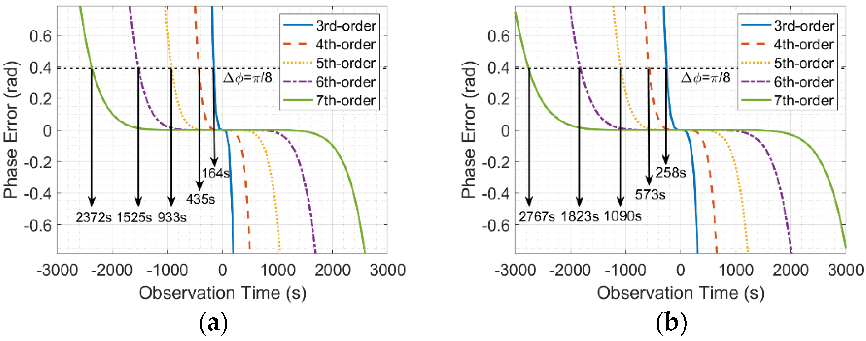
As the azimuth resolution increases, the low-order Taylor expansion range model shows insufficient accuracy in ultralong integration time.

(2)

The iterative approximation range model has a high accuracy but cannot be expressed by an analytical expression.

(3)

The range models lack the flexibility of precision adjustment for different exposure times.

The above problems are what this paper is dedicated to solving. This paper is organized as follows. In Section 2, there is a brief explanation of the invalidation of “stop-and-go” assumption, then the integration time of GEO SAR at different azimuth resolutions and fitting effects of several “non-stop-and-go” range models are shown. In Section 3, a novel range model based on the mth-order Taylor expansion is put forward, and the derivation of the pulse transmitting and receiving distance are given, respectively. Section 4 shows the simulation results of fitting errors and imaging results, based on several slant range models, which validate the effectiveness of the proposed range model in this paper. Section 5 gives conclusions.

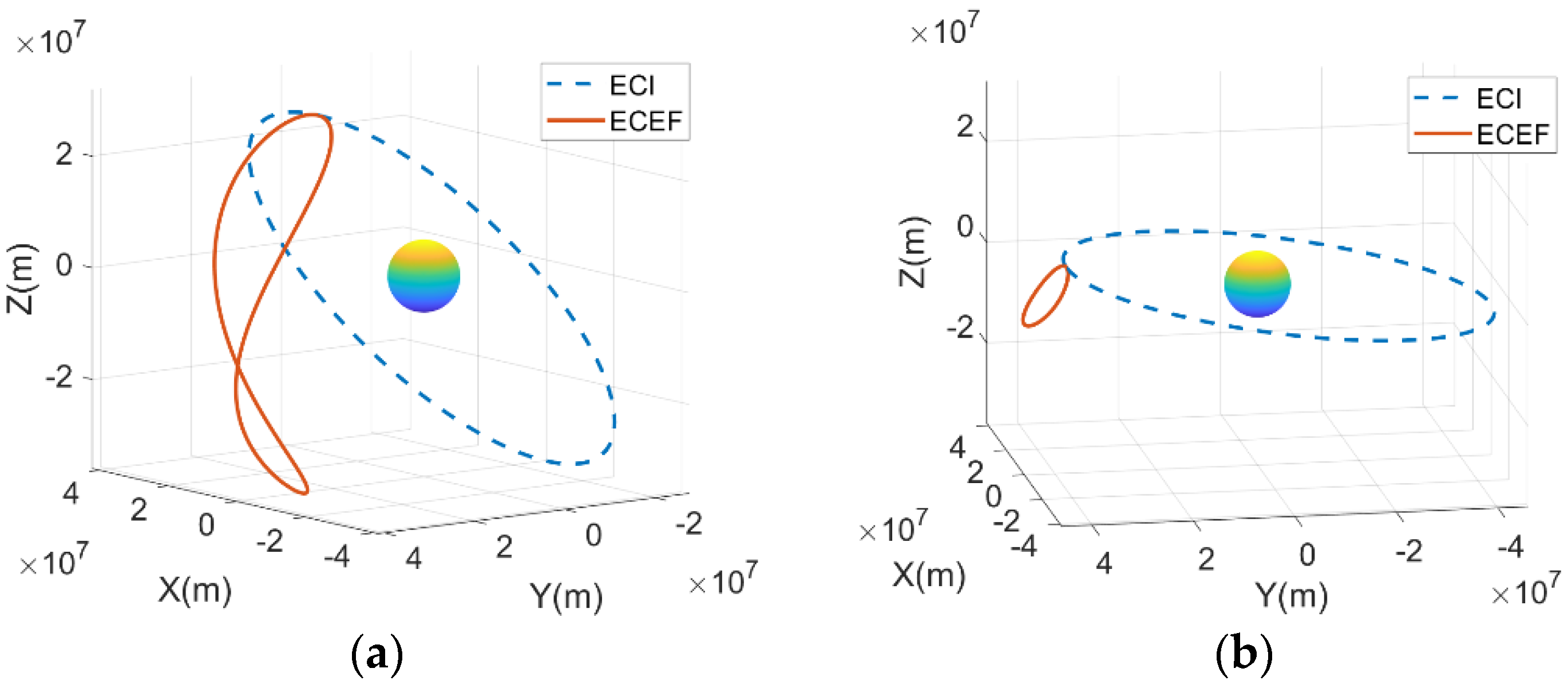
2. Characteristics of GEO SAR

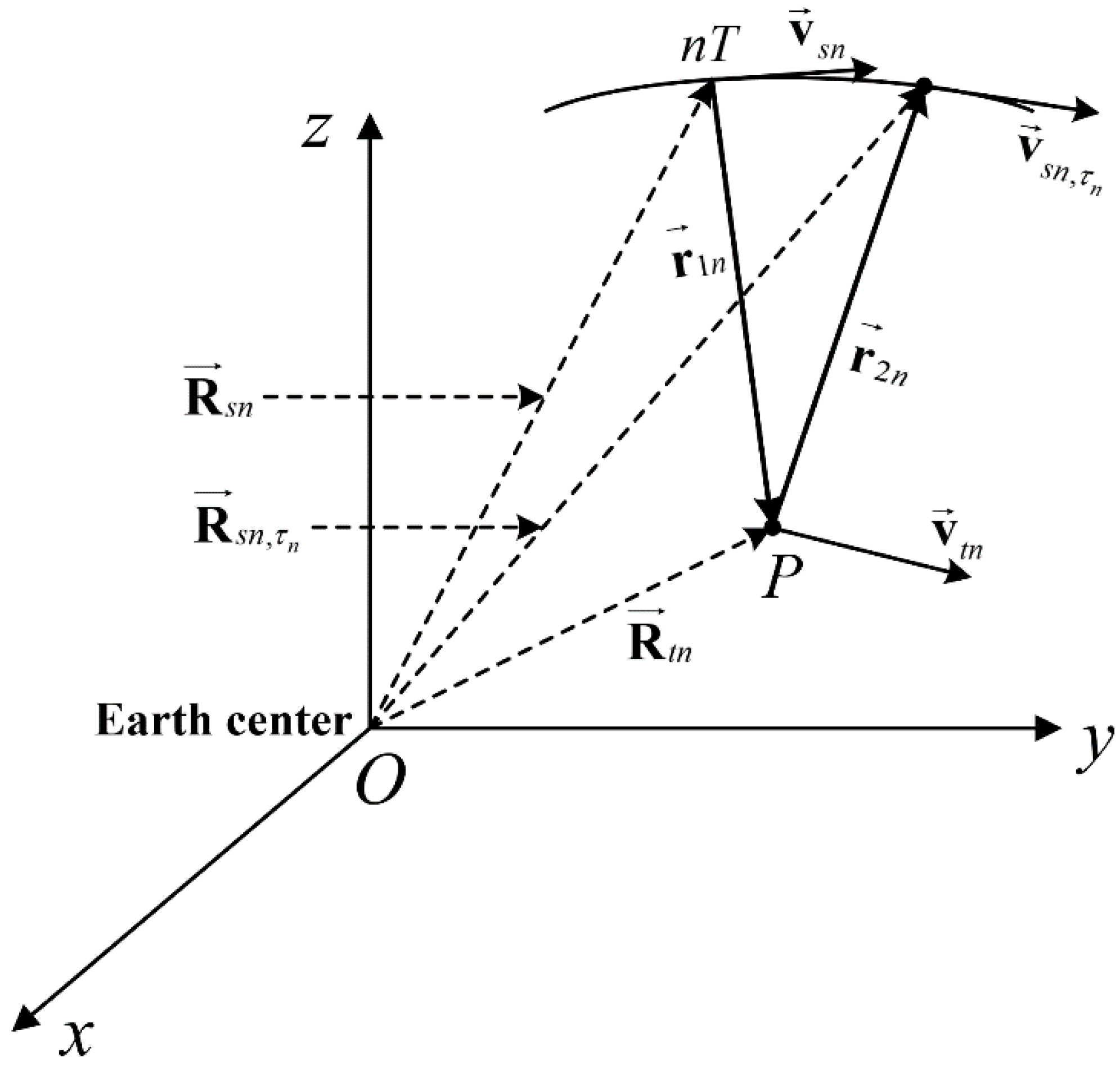
2.1. Invalidation of “Stop-and-Go” Assumption

The “stop-and-go” assumption is widely used in classic SAR imaging algorithms, which assumes that the radar platform and targets are relatively stationary, during pulse propagation. According to this hypothesis, the total propagation distance can be calculated as twice the instantaneous slant range between the antenna phase center and the target, at the time of pulse transmission. Nevertheless, this assumption ignores the range errors introduced by two forms of motion, one is the movement of platform relative to the target during pulse transmission and reception, and the other is the movement of platform relative to the target during pulse propagation. Figure 1 illustrates the GEO SAR pulse propagation model in an Earth-centered Earth-fixed (ECEF) coordinate system.

The first kind of error is determined by the radar system, which can be ignored when the pulse width is short enough. In GEO SAR signal processing, the second movement has a greater impact on the calculation of the slant range between the radar and target, especially when the integration time is very long. The propagation delays of the geosynchronous orbit satellite are always longer than 200 ms, during this period, the satellite runs along the orbit and the target is also displaced due to the rotation of the earth and its own motion. Thus, the range error caused by the “stop-and-go” assumption cannot be ignored.

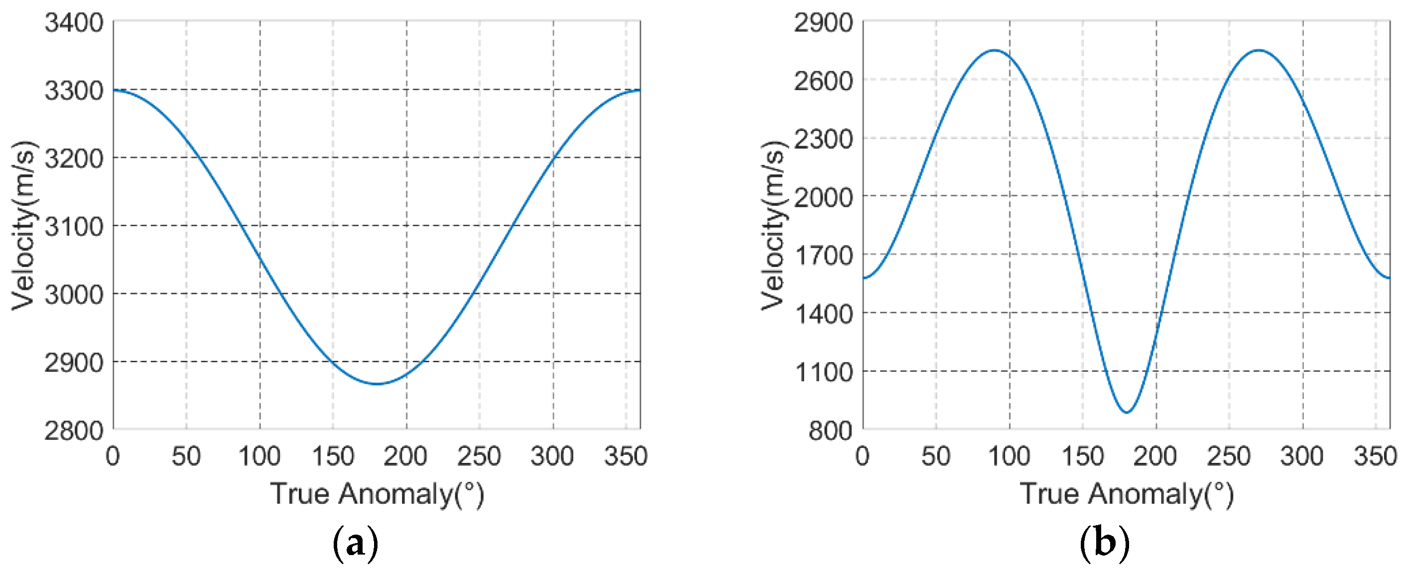
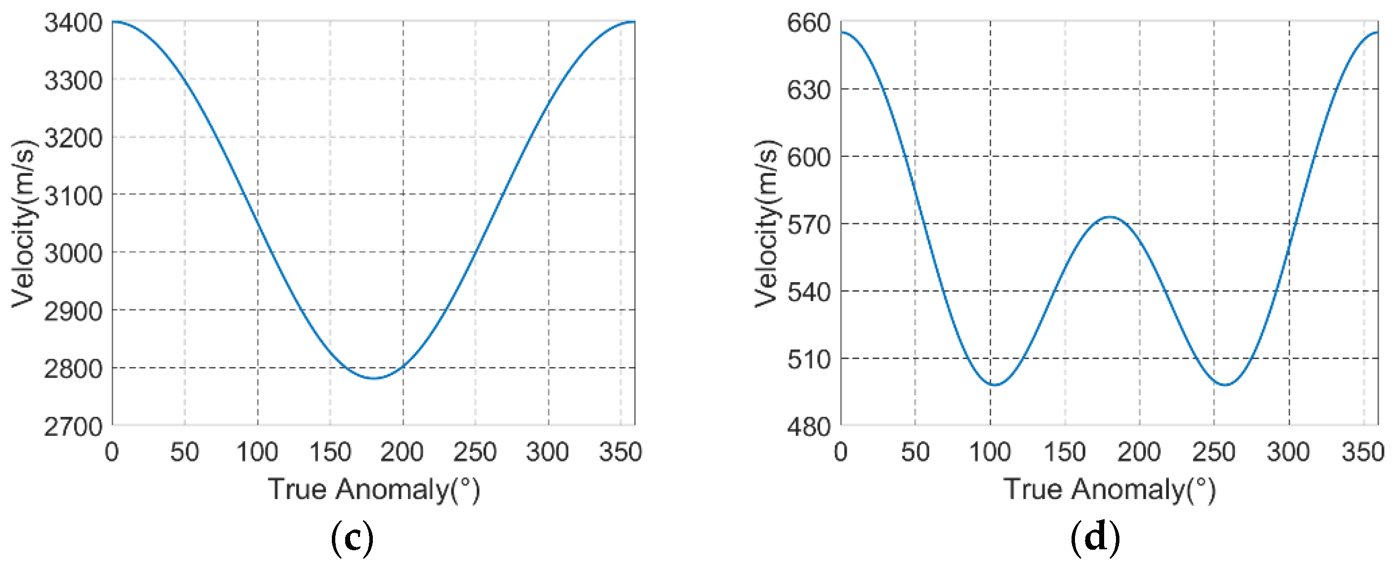
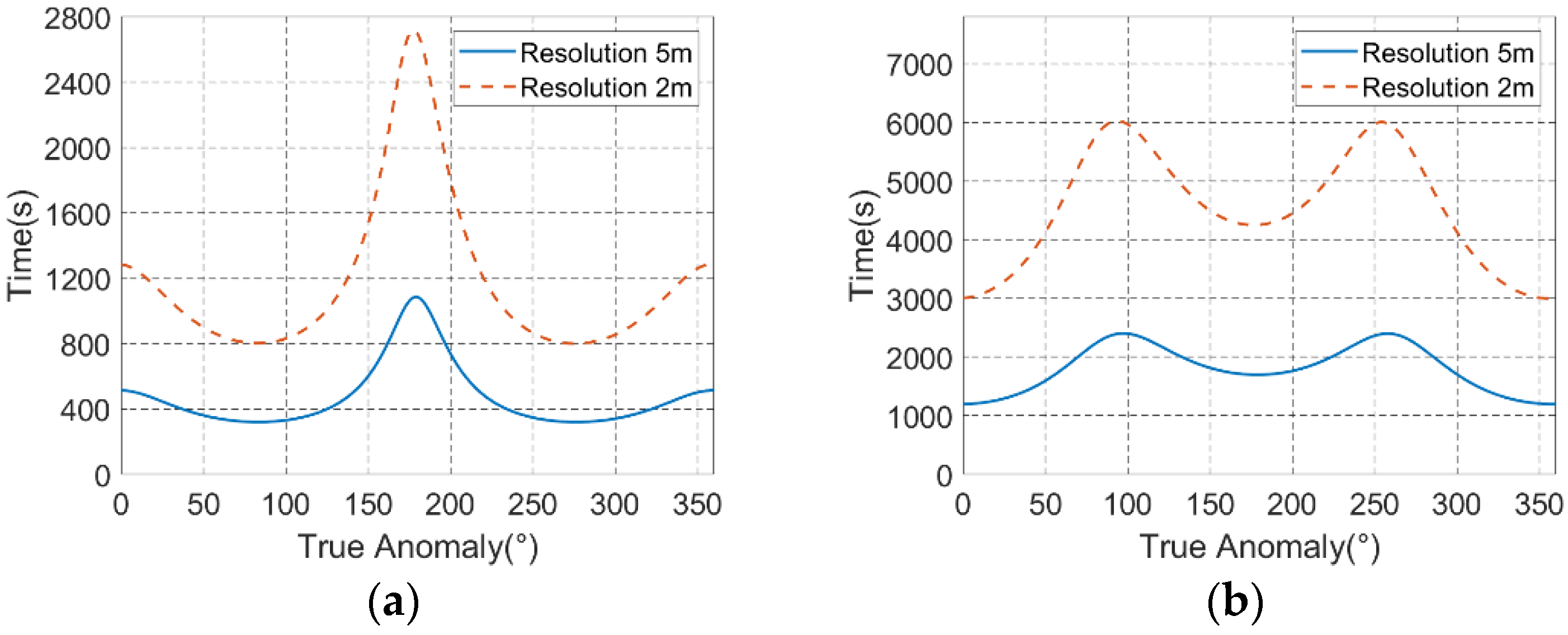
2.2. Ultralong Integration Time

The azimuth resolution of SAR is determined by the angle of synthetic aperture, so a SAR system always needs a longer integration time to obtain the same resolution on a higher orbit. A classic formula for calculating the integration time of different azimuth resolution can be expressed as follows:

$$T_{sar}=\frac{R\left({\eta }_c\right){\theta }_{syn}}{v_{ecef}}$$

(1)

where $R\left({\eta }_c\right)$ denotes the slant range at the center of the aperture, ${\theta }_{syn}$ is the angle of synthetic aperture, and $v_{ecef}$ is the velocity of the platform in the ECEF coordinate system. Unlike LEO SAR and airborne SAR, the velocity of GEO SAR satellite is quite different in the Earth-centered inertial (ECI) coordinate and the ECEF coordinate. This is mainly because the velocity of the satellite decreases as the orbital height increases, which causes the effect of the earth’s rotation to become more and more obvious.

However, Equation (1) is inaccurate for GEO SAR because of the complicated space trajectory and velocity changes. To illustrate this problem, we simulated the GEO SAR space trajectory and velocity under two orbital configurations. The simulation parameters are shown in

Table 1. Simulation parameters of GEO SAR.

Parameter	Value	Parameter	Value
Semi-major Axis	42,164 km	RAAN 1	0°
Inclination	53°/7.4°	Argument of Perigee	270°
Eccentricity	0.07/0.1	Down Angle	4.65°
PRF	70 Hz/140 Hz	Wave Length	0.24 m
Bandwidth	75 MHz /150 MHz	Pulsewidth	20 μs

¹ RAAN = Right Ascension of Ascending Node.

.

In Table 1, the orbital inclination of 53° and the eccentricity of 0.07 corresponds to the classic “8” shaped orbit, and the inclination of 7.4° and the eccentricity of 0.1 corresponds to a near-circular orbit, which is introduced in [12]. The simulation results of trajectory and velocity under these two orbit configurations are shown in Figure 2 and Figure 3.

It could be seen that the trajectory of GEO SAR in the ECEF coordinate always presents to be a complex spatial curve, and the shape of the trajectory is determined by the orbital parameters. Common shapes include “8” shaped, drop-shaped, and ellipse. From Figure 3, the velocity of GEO SAR in the ECEF coordinate is much lower than that of LEO SAR, which means that the integration time is seriously increased.

Considering that (1) will introduce an intolerable error when used for calculating the integration time of GEO SAR, we propose an accurate search method based on dichotomy. The basic steps can be briefly described as follows:

• Set an initial search region [T_min, T_max] according to the estimated integration time by (1), and this region is required to include the real integration time.
• Define T_mid = (T_min + T_max)/2. If T_max − T_min is smaller than the threshold, then return the T_real = T_mid and stop the iteration.
• Calculate the synthetic aperture angle of different exposure time T_min, T_max, and T_mid, denoted as θ_min, θ_max, and θ_mid.
• Define the new search region: if θ_mid > θ_syn, then T_max = T_mid, else let T_min = T_mid. Return to step 2.

Through the above steps, an accurate integration time can be obtained, its accuracy is controlled by the interval threshold, which can be selected according to the error requirements. The interval threshold is selected as 1 s in this experiment, and the simulation results are shown in Figure 4.

According to Figure 4, the integration time of the classic “8” shaped orbit is shorter than that of the near-circular orbit, but the maximum integration time also reaches 1086 s at 5 m azimuth resolution. As for the near-circular orbit, the maximum integration time even reaches 2400 s at the same resolution. Regarding 2 m azimuth resolution, the integration time becomes much longer. Therefore, whether the existing range models can be applied to such a long imaging time remains to be verified.

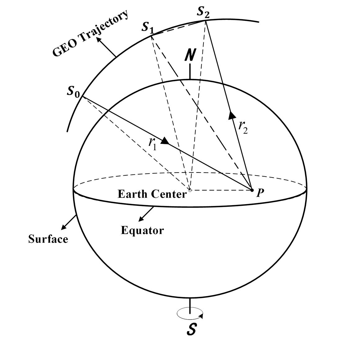
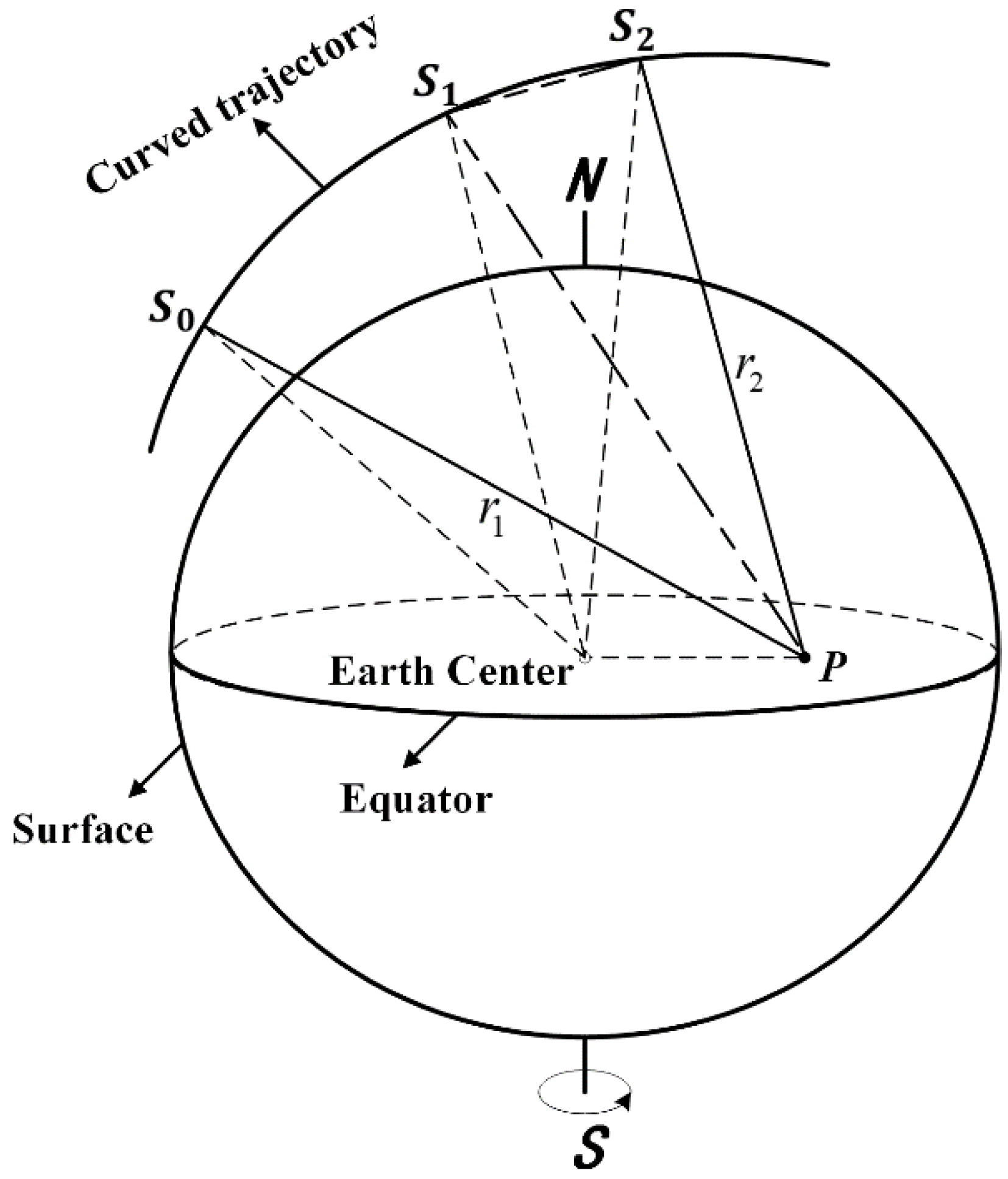
2.3. “Non-Stop-and-Go” Range Models

With the continuous deepening of GEO SAR research, many scholars proposed their own range models, which took the “stop-and-go” assumption failure into account [31,32,33,34,35]. In order to analyze the applicability of these models for long integration times, a series of fitting experiments were conducted. The parameters used in simulation are shown in Table 1, the observation time was chosen as 2000 s, and the “8” shaped orbit was selected for this experiment. The phase error simulation results of the whole orbit are shown in Figure 5 and

Table 2. Fitting error comparison of several GEO SAR range models.

Range Model	Mean Error (rad)	Max Error (rad)	Standard Deviation (rad)
“Stop-and-go” assumption	47.29	153.72	12.79
Fourth-order Taylor expansion	3.95	50.56	4.41
Iterative approximation	1.84 × 10−6	1.21 × 10−5	1.16 × 10−6

. Among these figures, x-axis is the observation time, y-axis is the true anomaly, and z-axis is the phase error between these range models and the real propagation distance.

In order to get the fitting error of these range models, we also need to know the real distance of pulse propagation. Considering that the equation about the real distance is a transcendental equation and has no analytical solution, a dichotomy search method is used to approximate it. The specific calculation process is described in [36].

According to Figure 5, a simple summary of these two “non-stop-and-go” range models can be made:

(1)

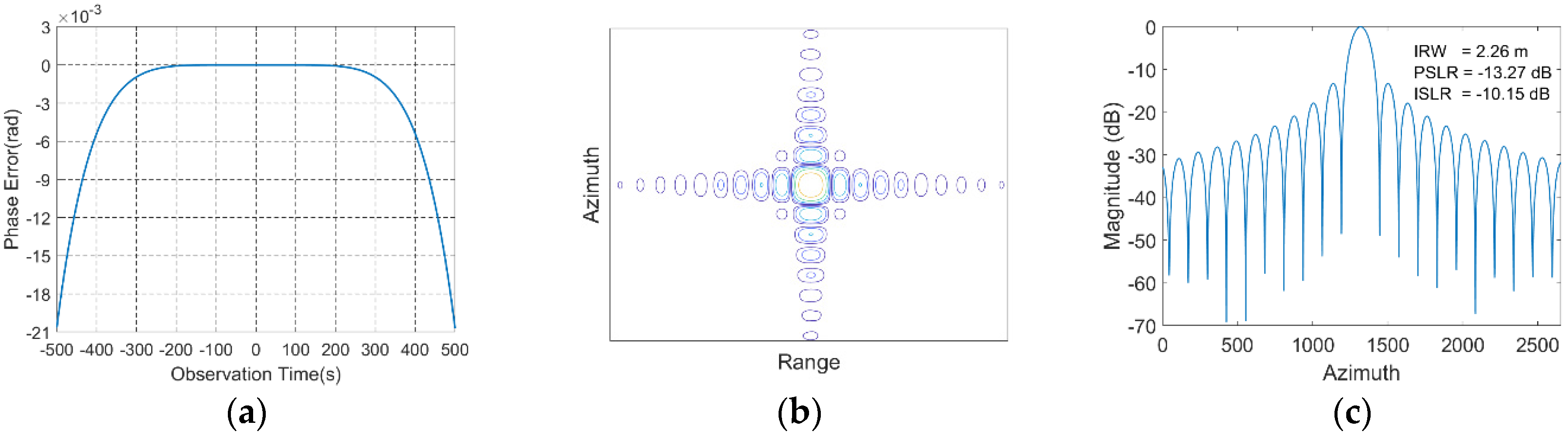
Fourth-order Taylor expansion model considering the invalidation of “stop-and-go” assumption. This model can be expressed in the form of a power series, which can obtain the 2-D spectrum to form an efficient frequency domain imaging algorithm. However, limited by the order of expansion, this model only has a satisfactory fitting effect in a short observation time. As the exposure time increases, the fitting error accumulates rapidly at both edges of the aperture.

(2)

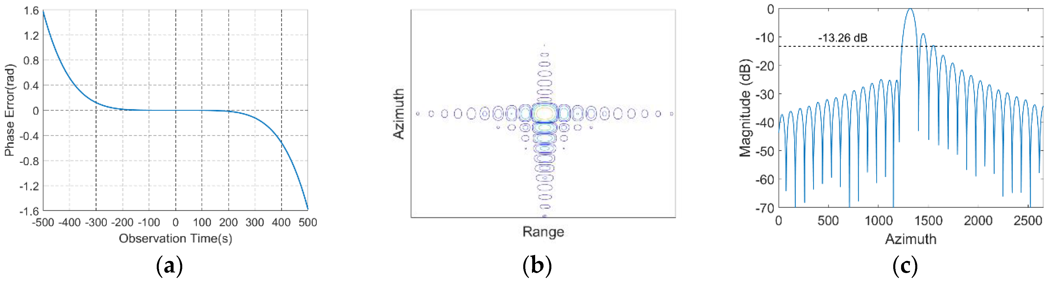
Iterative approximation range model. The main idea of this range model is to use twice the transmitting delay to approximately calculate the satellite position in the orbit, then an iteration can be formed to calculate a relatively accurate result. The calculation of this model is simple, and only one iteration already has a high accuracy, which can be used in echo generation and time-domain imaging algorithms. However, this range model cannot be expressed by an analytical expression, so its usage for frequency domain imaging algorithms is limited.

3. Proposed Range Model and Imaging Algorithm

3.1. Proposed Range Model

Based on the two “non-stop-and-go” GEO SAR range models introduced in Section 2, an improved range model is proposed, which mainly has the following two advantages:

(1)

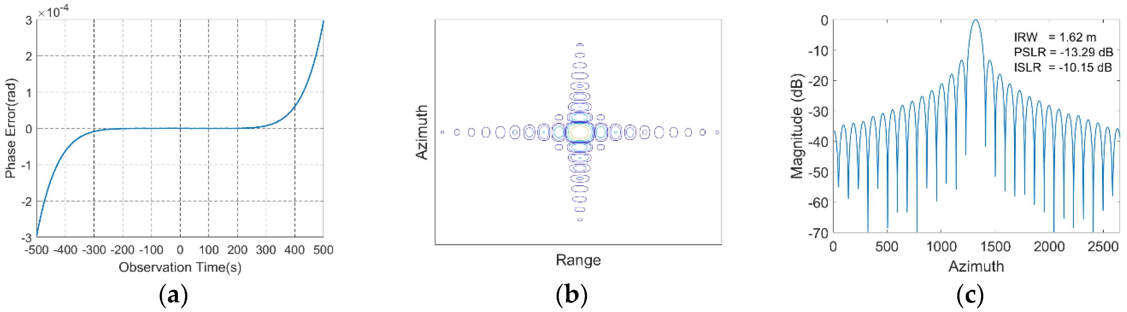
A general calculation method for mth-order expansion of pulse transmitting distance is given, and the expansion order can be adjusted according to the integration time and error accuracy requirement.

(2)

An accurate pulse receiving distance is obtained by using the thought of iterative approximation, and the analytical expression is obtained by Taylor expansion in the ECEF coordinate system.

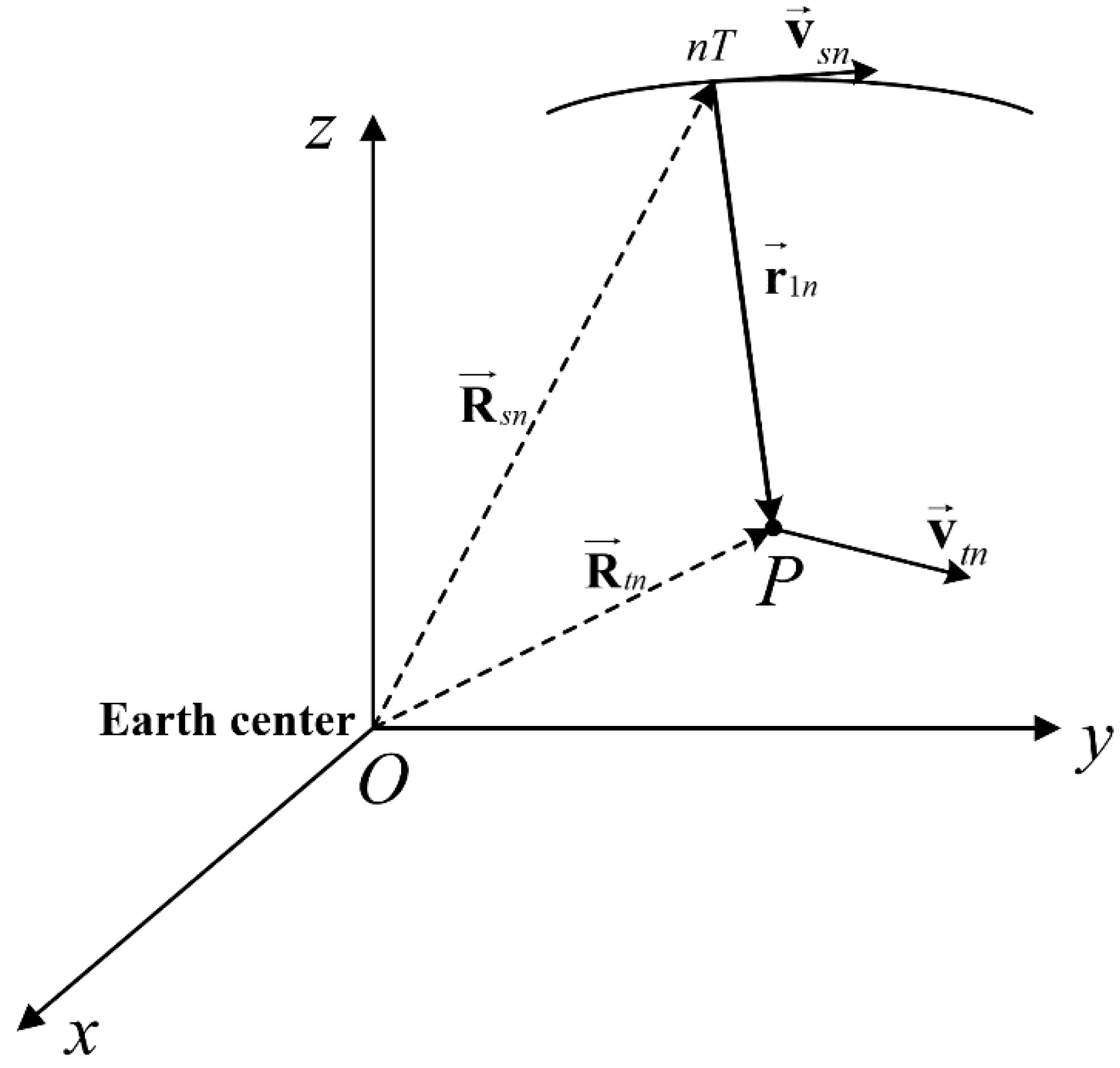
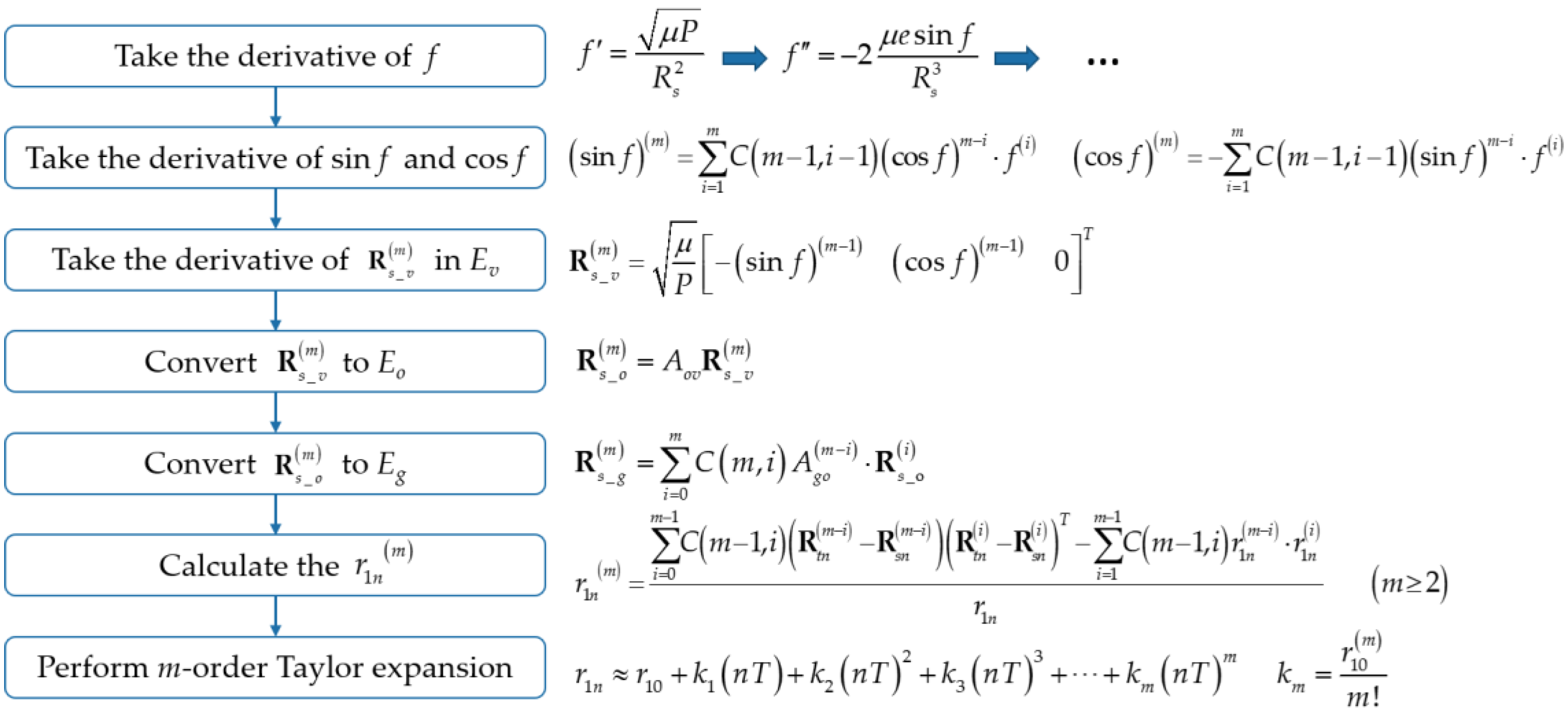
3.1.1. Pulse Transmitting Distance

This part introduces the mth-order Taylor expansion method of the pulse transmitting distance, and all the following derivation is completed in the ground-fixed coordinate system. Without loss of generality, assume that the ground target has a moving speed. Figure 6 shows the propagation history of the transmitted pulse at the nth pulse repetition time (PRT).

According to Figure 6, the pulse transmitting distance vector can be expressed as:

$$r_{1n}=R_{tn}-R_{sn}$$

(2)

To derive the modulus of r_1n, we can first square the two sides of Equation (2),

$${\Vert r_{1n}\Vert }^2=\left(R_{tn}-R_{sn}\right){\left(R_{tn}-R_{sn}\right)}^T$$

(3)

Taking the derivative of Equation (3), the first-derivative and second-derivative of the transmitting distance can be obtained:

$$r_{1n}{}^{\prime }=\frac{\left(V_{tn}-V_{sn}\right)r_{1n}^T}{r_{1n}}$$

(4)

$$r_{1n}{}^{″}=\frac{\left(A_{tn}-A_{sn}\right)r_{1n}^T+{\Vert V_{tn}-V_{sn}\Vert }^2-{\left(r_{1n}{}^{\prime }\right)}^2}{r_{1n}}$$

(5)

where A_sn and A_tn are the acceleration of satellite and target, respectively.

Then, the high order derivatives of transmitting distance can be achieved by taking the derivative of Equation (5) step by step. In order to make the formula concise and easy to find the rules, the results of previous derivative are substituted into the next expression. The derivatives from the third-order to the fifth-order can be expressed as follows:

$$r_{1n}{}^{\left(3\right)}=\frac{\left(R_{tn}^{\left(3\right)}-R_{sn}^{\left(3\right)}\right)r_{1n}{}^T+3\left({R^{″}}_{tn}-{R^{″}}_{sn}\right){\left({R^{\prime }}_{tn}-{R^{\prime }}_{sn}\right)}^T+3r_{1n}{}^{″}\cdot r_{1n}{}^{\prime }}{r_{1n}}$$

(6)

$$r_{1n}{}^{\left(4\right)}=\frac{\left(R_{tn}^{\left(4\right)}-R_{sn}^{\left(4\right)}\right)r_{1n}{}^T+4\left(R_{tn}^{\left(3\right)}-R_{sn}^{\left(3\right)}\right){\left({R^{\prime }}_{tn}-{R^{\prime }}_{sn}\right)}^T+3{\Vert {R^{″}}_{tn}-{R^{″}}_{sn}\Vert }^2-4r_{1n}^{\left(3\right)}\cdot r_{1n}{}^{\prime }+3{\left(r_{1n}{}^{″}\right)}^2}{r_{1n}}$$

(7)

$$r_{1n}{}^{\left(5\right)}=\frac{\left(R_{tn}^{\left(5\right)}-R_{sn}^{\left(5\right)}\right)r_{1n}{}^T+5\left(R_{tn}^{\left(4\right)}-R_{sn}^{\left(4\right)}\right){\left({R^{\prime }}_{tn}-{R^{\prime }}_{sn}\right)}^T+10\left(R_{tn}^{\left(3\right)}-R_{sn}^{\left(3\right)}\right){\left({R^{″}}_{tn}-{R^{″}}_{sn}\right)}^T-5r_{1n}^{\left(4\right)}\cdot r_{1n}{}^{\prime }+10r_{1n}^{\left(3\right)}\cdot r_{1n}{}^{″}}{r_{1n}}$$

(8)

According to the above equations and binomial expansion, the general formula of the mth-order derivative of the transmitting distance can be written in the following form:

$$r_{1n}{}^{\left(m\right)}=\frac{{\displaystyle \sum _{i=0}^{m-1}C\left(m-1,i\right)\left(R_{tn}^{\left(m-i\right)}-R_{sn}^{\left(m-i\right)}\right){\left(R_{tn}^{\left(i\right)}-R_{sn}^{\left(i\right)}\right)}^T-{\displaystyle \sum _{i=1}^{m-1}C\left(m-1,i\right)r_{1n}^{\left(m-i\right)}\cdot r_{1n}^{\left(i\right)}}}}{r_{1n}} \left(m\ge 2\right)$$

(9)

where $C\left(m-1,i\right)$ represents the combination formula.

After obtaining the high order derivatives, the mth-order Taylor expansion of the transmitting distance can be performed at the beam center moment:

$$\begin{array}{c}{r}_{1n}\approx r_{10}+r_{10}{}^{\prime }\left(nT\right)+\frac{r_{10}{}^{″}}{2}{\left(nT\right)}^2+\frac{r_{10}{}^{‴}}{6}{\left(nT\right)}^3+\cdots +\frac{r_{10}^{\left(m\right)}}{m!}{\left(nT\right)}^m\\ =r_{10}+k_1\left(nT\right)+k_2{\left(nT\right)}^2+k_3{\left(nT\right)}^3+\cdots +k_m{\left(nT\right)}^m\end{array}$$

(10)

where nT is the azimuth time, and k_m represents the mth-order coefficient of azimuth time.

In order to calculate the mth-order derivative of transmitting distance, first, we need to find the first-order to mth-order derivatives of R_sn and R_tn. Considering that the motion state of the target is known already, the key point to this problem lies in the derivative of the satellite position vector. During the calculation process, we found that the mth-order derivative of R_sn has a form that is easy to represent and iteratively calculate in the orbital coordinate system. Therefore, the derivatives of R_sn is first calculated in the orbital coordinate system, and are then rotated into the ECEF coordinate system. For convenience, the three coordinate systems used in the subsequent derivation are defined here—E_v represents the orbital coordinate system, E_o represents the ECI coordinate system, and E_g represents the ECEF coordinate system.

According to the orbit equation, the satellite velocity vector in the orbit coordinate system E_v can be expressed as:

$$V_{s\_v}=\sqrt{\frac{\mu }{P}}{\left[\begin{array}{ccc}-\sin f& e+\cos f & 0\end{array}\right]}^{\mathrm{T}}$$

(11)

where f is the true anomaly, μ is the geocentric gravitational constant, μ = 3.986005 × 10¹⁴ m³/s², P and e are the semi-latus rectum and the eccentricity of the orbit.

Taking sin f and cos f as a whole, the mth-order derivative of the satellite position vector can be expressed as:

$$R_{s\_v}^{\left(m\right)}=\sqrt{\frac{\mu }{P}}{\left[-{\left(\sin f\right)}^{\left(m-1\right)} {\left(\cos f\right)}^{\left(m-1\right)} 0\right]}^T$$

(12)

$$\{\begin{array}{l}{\left(\sin f\right)}^{\left(m\right)}={\displaystyle \sum _{i=1}^{m}C\left(m-1,i-1\right){\left(\cos f\right)}^{m-i}\cdot f^{\left(i\right)}}\\ {\left(\cos f\right)}^{\left(m\right)}=-{\displaystyle \sum _{i=1}^{m}C\left(m-1,i-1\right){\left(\sin f\right)}^{m-i}\cdot f^{\left(i\right)}}\end{array}$$

(13)

According to Equations (12) and (13), if the 1st to (m − 1)-th order derivatives of true anomaly are obtained, the mth-order derivative of the satellite position vector in E_v can be obtained. The first-order to fifth-order derivatives of f are given in Appendix A.

Next is the coordinate rotation part. First, rotate the mth-order derivative of R_{s_v} from E_v to E_o. Considering that the rotation matrix A_ov is constant, it can be directly written as:

$$R_{s\_o}^{\left(m\right)}=A_{ov}{R}_{s\_v}^{\left(m\right)}$$

(14)

$$A_{ov}=\left[\begin{array}{ccc}\cos {\Omega }& -\sin {\Omega }& 0\\ \sin {\Omega }& \cos {\Omega }& 0\\ 0& 0& 1\end{array}\right]\left[\begin{array}{ccc}1& 0& 0\\ 0& \cos {\theta }_i& -\sin {\theta }_i\\ 0& \sin {\theta }_i& \cos {\theta }_i\end{array}\right]\left[\begin{array}{ccc}\cos \omega & -\sin \omega & 0\\ \sin \omega & \cos \omega & 0\\ 0& 0& 1\end{array}\right]$$

(15)

Second, rotate the mth-order derivative of R_{s_o} from E_o to E_g. However, the rotation matrix A_go has the variable orbit time t_s, so we also need to take the derivative of A_go.

The rotation matrix A_go can be written as:

$$A_{go}=\left[\begin{array}{ccc}\cos H_g& \sin H_g& 0\\ -\sin H_g& \cos H_g& 0\\ 0& 0& 1\end{array}\right]$$

(16)

$$H_g={\omega }_e\cdot t_s$$

(17)

where H_g is the Greenwich hour angle, ω_e is the angular velocity of the earth’s rotation, t_s is the Greenwich mean time. The mth-order derivative of A_go can be expressed as:

$$A_{go}^{\left(m\right)}={\omega }_e^m\left[\begin{array}{ccc}\cos \left(H_g+\frac{m\pi }{2}\right)& \sin \left(H_g+\frac{m\pi }{2}\right)& 0\\ -\sin \left(H_g+\frac{m\pi }{2}\right)& \cos \left(H_g+\frac{m\pi }{2}\right)& 0\\ 0& 0& 0\end{array}\right]m\ge 1$$

(18)

Therefore, the mth-order derivative of satellite position vector in E_g can be written as follows:

$$R_{s\_g}^{\left(m\right)}={\displaystyle \sum _{i=0}^{m}C\left(m,i\right)A_{go}^{\left(m-i\right)}\cdot R_{s\_o}^{\left(i\right)}}$$

(19)

From the above, the complete calculation process of the mth-order Taylor expansion of transmitting distance is given, and Figure 7 summarizes the process of calculation.

3.1.2. Pulse Receiving Distance

According to the analysis and simulation results in Section 2, the “stop-and-go” hypothesis is invalid in GEO SAR. Therefore, it is inaccurate to approximate the pulse receiving distance with the transmitting distance. In view of the fact that the iterative approximation range model has a high accuracy but cannot be expressed by an analytical expression, a new calculation method of pulse receiving distance is proposed in this paper, which combines the Taylor expansion with one iteration approximation. Figure 8 shows the propagation history of transmitting and receiving pulse at the nth PRT in the ECEF coordinate system.

The relationship between pulse transmitting distance and receiving distance can be expressed as:

$$\{\begin{array}{l}{r}_{1n}=\Vert r_{1n}\Vert =\Vert R_{tn}-R_{sn}\Vert \\ r_{2n}=\Vert r_{2n}\Vert =\Vert R_{sn,{\tau }_n}-R_{tn}\Vert =\Vert R_{sn}+V_{sn}{\tau }_n-R_{tn}\Vert \end{array}$$

(20)

Similar to the transmitting distance, the first-order and second-order derivatives of the receiving distance can be expressed as:

$$r_{2n}{}^{\prime }=\frac{\left(A_{sn}{\tau }_n+V_{sn}-V_{tn}\right){\left(V_{sn}{\tau }_n-r_{1n}\right)}^T}{r_{2n}}$$

(21)

$$r_{2n}{}^{″}=\frac{\left(R_{sn}^{\left(3\right)}{\tau }_n+A_{sn}-A_{tn}\right){\left(V_{sn}\tau -r_{1n}\right)}^T+{\Vert A_{sn}{\tau }_n+V_{sn}-V_{tn}\Vert }^2-{\left({r^{\prime }}_{2n}\right)}^2}{r_{2n}}$$

(22)

The general formula of the mth-order derivative of the pulse receiving distance can be written in the following form:

$$r_{2n}{}^{\left(m\right)}=\frac{{\displaystyle \sum _{i=0}^{m-1}C\left(m-1,i\right)\left(R_{sn}^{\left(m+1-i\right)}{\tau }_n+R_{sn}^{\left(m-i\right)}-R_{tn}^{\left(m-i\right)}\right){\left(R_{sn}^{\left(i+1\right)}{\tau }_n+R_{sn}^{\left(i\right)}-R_{tn}^{\left(i\right)}\right)}^T-{\displaystyle \sum _{i=1}^{m-1}C\left(m-1,i\right)r_{2n}^{\left(m-i\right)}\cdot r_{2n}^{\left(i\right)}}}}{r_{2n}}\left(m\ge 2\right)$$

(23)

Considering that the pulse propagation time τ_n is subsecond, its higher order terms have little effect on the fitting error. Therefore, this paper only performs a second-order Taylor expansion of the receiving distance on fast time, and the subsequent simulations in Section 4 also prove that the second-order expansion can achieve sufficiently high accuracy.

Performing the fast-time Taylor expansion of the receiving distance at a pulse transmitting time, that is, τ equal to 0, the expansion can be written as:

$$r_{2n}\approx r_{1n}+r_{1n}{}^{\prime }{\tau }_n+\frac{r_{1n}{}^{″}}{2}{\tau }_n^2$$

(24)

In view of the fact that the actual value of the total pulse propagation time τ_n cannot be solved, the idea of one iteration approximation is employed here. The total propagation time is replaced by double the transmitting delay:

$${\tau }_n\approx \frac{2r_{1n}}{c}$$

(25)

It should be pointed out that this approximation step implies the upper limit of the fitting performance of this method, its fitting error would not be better than that of the iterative approximation range model.

Substituting the approximate propagation time into Equation (24), the first-order term can be expressed as:

$$\begin{array}{ll}\frac{\left(V_{tn}-V_{sn}\right)r_{1n}{}^T}{r_{1n}}{\tau }_n& \approx \frac{\left(V_{tn}-V_{sn}\right)r_{1n}{}^T}{r_{1n}}\frac{2r_{1n}}{c}=2\frac{\left(V_{tn}-V_{sn}\right)r_{1n}{}^T}{c}\\ & =2{\Delta }{r}_1\end{array}$$

(26)

Then, the slow-time Taylor expansion of ${\Delta }{r}_1$ is performed at the beam center moment:

$${\Delta }{r}_1\approx {\Delta }{r}_{10}+{\Delta }{k}_{11}\left(nT\right)+{\Delta }{k}_{12}{\left(nT\right)}^2+\cdots +{\Delta }{k}_{1m}{\left(nT\right)}^m$$

(27)

$$\{\begin{array}{l}{\Delta }{r}_{10}=\frac{\left(V_{s0}-V_{t0}\right)r_{10}{}^T}{c}\\ {\Delta }{k}_{1m}=\frac{{\displaystyle \sum _{i=0}^{m}C\left(m,i\right)\left(R_{s0}^{\left(m-i+1\right)}-R_{t0}^{\left(m-i+1\right)}\right){\left(R_{t0}^{\left(i\right)}-R_{s0}^{\left(i\right)}\right)}^T}}{c\cdot m!}m\ge 1\end{array}$$

(28)

Considering that the first-order term is the main source of the fitting error, it should be expanded to a specified order, according to the accuracy requirements in actual use. In the following simulation of this paper, the fifth-order expansion of ${\Delta }{r}_1$ proved to have a sufficiently high accuracy.

Next, repeating the same steps, the second-order term can be expressed as:

$$\begin{array}{ll}& \frac{{\tau }_n^2}{2}\frac{\left(A_{tn}-A_{sn}\right)r_{1n}{}^T+{\Vert V_{tn}-V_{sn}\Vert }^2-{\left({r^{\prime }}_{2n}\right)}^2}{r_{1n}}\\ \approx & \frac{2}{c^2}\left[r_{1n}\left[\left(A_{tn}-A_{sn}\right)r_{1n}{}^T+{\Vert V_{tn}-V_{sn}\Vert }^2\right]-\frac{{\left[\left(V_{tn}-V_{sn}\right)r_{1n}{}^T\right]}^2}{r_{1n}}\right]\\ =& 2{\Delta }{r}_2\end{array}$$

(29)

Similar to the expansion of ${\Delta }{r}_1$, the slow-time Taylor expansion of ${\Delta }{r}_2$ is performed at the beam center moment:

$${\Delta }{r}_2\approx {\Delta }{r}_{20}+{\Delta }{k}_{21}\left(nT\right)+{\Delta }{k}_{22}{\left(nT\right)}^2+\cdots +{\Delta }{k}_{2m}{\left(nT\right)}^m$$

(30)

Given that ${\Delta }{r}_2$ is the second-order term of fast-time, it has less impact on the fitting error. Therefore, only the first-order expansion is sufficient to ensure the fitting accuracy. The calculation results of the ${\Delta }{r}_{20}$ and ${\Delta }{r}_{21}$ are as follows:

$${\Delta }{r}_{20}=\frac{1}{c^2}\left[r_{10}\left(\left(A_{t0}-A_{s0}\right)r_{10}^T+{\Vert V_{t0}-V_{s0}\Vert }^2\right)-\frac{{\left(\left(V_{tn}-V_{sn}\right)r_{10}^T\right)}^2}{r_{10}}\right]$$

(31)

$$\begin{array}{ll}{\Delta }{k}_{21}& =\frac{r_{10}}{c^2}\left[\left(R_{t0}^{\left(3\right)}-R_{s0}^{\left(3\right)}\right)r_{10}^T+3\left(A_{t0}-A_{s0}\right){\left(V_{t0}-V_{s0}\right)}^T\right]+\frac{{r^{\prime }}_{10}}{c^2}[\left(\left(A_{t0}-A_{s0}\right)r_{10}^T+{\Vert V_{t0}-V_{s0}\Vert }^2\right)\\ & -\frac{2}{r_{10}\cdot c^2}\left[\left(V_{t0}-V_{s0}\right)r_{10}^T\right]\left[\left(A_{t0}-A_{s0}\right)r_{10}^T+{\Vert V_{t0}-V_{s0}\Vert }^2\right]+\frac{{r^{\prime }}_{10}}{r_{10}^2\cdot c^2}{\left[\left(V_{t0}-V_{s0}\right)r_{10}^T\right]}^2\end{array}$$

(32)

From the above, after considering the failure of “stop-and-go” assumption, the pulse receiving distance can be expanded as:

$$\begin{array}{ll}{r}_{2n}& =r_{1n}+{\Delta }r\approx r_{1n}+2{\Delta }{r}_1+2{\Delta }{r}_2\\ & =r_{1n}+2\left[\left({\Delta }{r}_{10}+{\Delta }{r}_{20}\right)+\left({\Delta }{k}_{11}+{\Delta }{k}_{21}\right)\left(nT\right)+{\Delta }{k}_{12}{\left(nT\right)}^2+\cdots +{\Delta }{k}_{15}{\left(nT\right)}^5\right]\end{array}$$

(33)

3.1.3. Total Pulse Propagation Distance

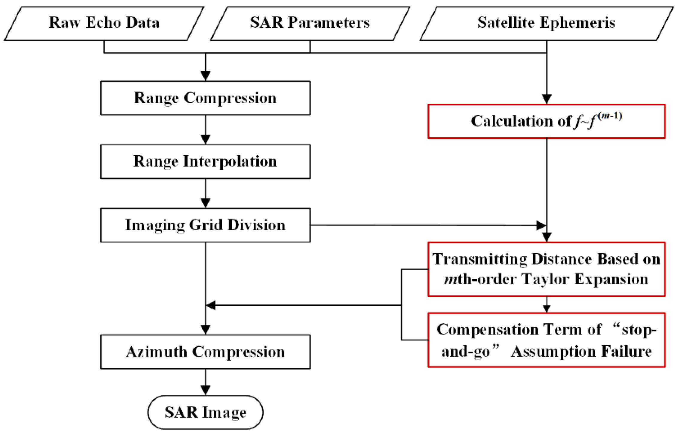
The first part of this section introduces a general method to calculate the mth-order Taylor expansion of pulse transmitting distance in GEO SAR, whose expansion order can be adjusted by the accuracy requirement and integration time. The second part illustrates an approach to approximately calculate the pulse receiving distance based on twice Taylor expansion, the first expansion is for fast-time and the other is for slow-time. In addition, all derivation of this range model is based on a ground moving target, so this model is also applicable to the moving target.

Based on the derivation and analysis above, an accurate range model in GEO SAR, which considers the invalidation of “stop-and-go” assumption can be expressed as:

$$r_n=r_{1n}+r_{2n}=2r_{1n}+{\Delta }r\approx 2r_{1n}+2\left({\Delta }{r}_1+{\Delta }{r}_2\right)$$

(34)

$$\{\begin{array}{l}{r}_{1n}\approx r_{10}+k_1\left(nT\right)+k_2{\left(nT\right)}^2+k_3{\left(nT\right)}^3+\cdots +k_m{\left(nT\right)}^m\\ {\Delta }r\approx 2\left({\Delta }{r}_{10}+{\Delta }{r}_{20}+\left({\Delta }{k}_{11}+{\Delta }{k}_{21}\right)\left(nT\right)+\left({\Delta }{k}_{12}+{\Delta }{k}_{22}\right){\left(nT\right)}^2+\cdots +\left({\Delta }{k}_{1m}+{\Delta }{k}_{2m}\right){\left(nT\right)}^m\right)\end{array}$$

(35)

where r_1n and ${\Delta }r$ represents the Taylor expansion of the pulse transmitting distance and the compensation term for the “stop-and-go” error, respectively. The fitting precision of this range model for the ultralong integration time is mainly determined by r_1n, whose accuracy can be adjusted by the expansion order m. The calculation of ${\Delta }r$ mainly uses the ideas of iterative approximation and twice Taylor expansion, since the total propagation time is subsecond, there is often no need to expand ${\Delta }r$ to a very high order in actual use.

3.2. Imaging Method

Considering the curved trajectory and invalidation of the “stop-and-go” assumption of GEO SAR, the conventional imaging algorithms cannot be directly used for focusing. Based on the range model proposed in this paper, an improved back projection (BP) focusing algorithm is used for imaging [37,38]. Figure 9 shows the flowchart of the improved BP algorithm.

The main process of the algorithm is the same as that of traditional BP, and the differences are marked in the flowchart with red boxes. The main different steps are as follows:

(1)

Calculating the true anomaly and its derivatives from 1st to (m − 1)-th order based on the satellite ephemeris data and orbit configuration;

(2)

Determining the Taylor expansion order m by the SAR system parameters and error accuracy, and then performing the mth-order Taylor expansion to obtain the transmitting distance for each grid point.

(3)

Calculating the compensation term of the “stop-and-go” assumption failure, and then bringing the complete pulse propagation distance into the azimuth compression.

4. Simulation Results and Discussion

The range model proposed in this paper can be divided into two parts—pulse transmitting distance and compensation term for “stop-and-go” error. In order to verify the effectiveness of the proposed range model and analyze the impact of different terms on the fitting accuracy, this section gives some simulation results on pulse propagation distance fitting and point target focusing. The simulation parameters are shown in Table 1, and if there are none specifically mentioned below, the satellite orbit is an “8” shaped orbit. All targets are in the stationary state.

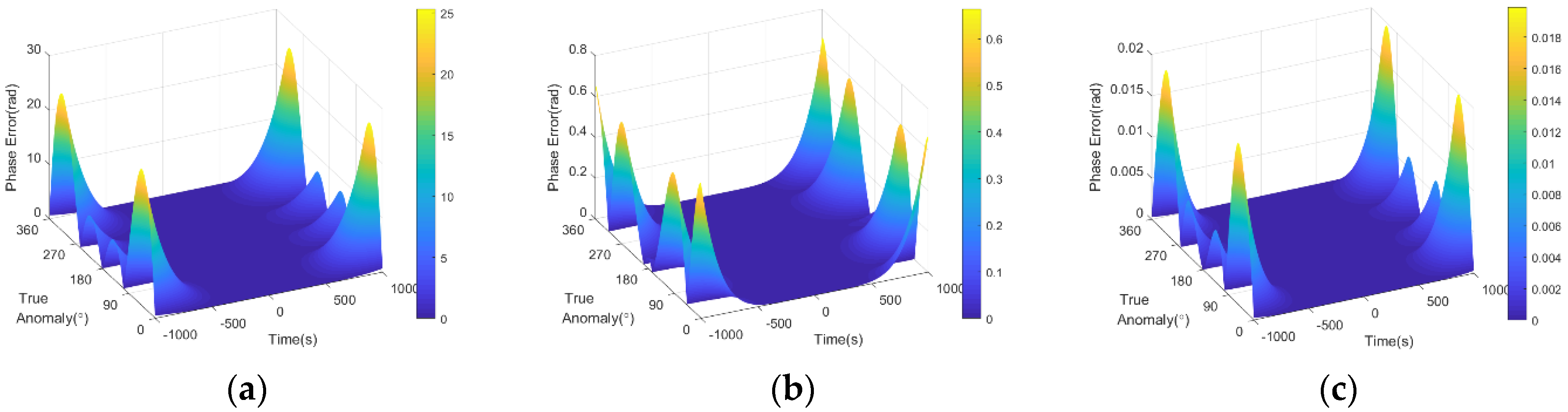
4.1. Fitting Error of the Pulse Transmitting Distance

This subsection focuses on simulating the fitting error of each order of Taylor expansion for different integration time, the simulation results can be helpful for selecting the expansion order of the range model. According to Equation (34), the final slant distance is composed of twice the transmitting distance and a compensation term, so the phase error of the transmitting distance should be at least less than $\pi /8$.

Figure 10 and

Table 3. Pulse transmitting distance fitting error comparison of different order Taylor expansion.

Expansion Order	Mean Error (rad)	Max Error (rad)	Standard Deviation (rad)
Fourth-order	1.97	25.28	2.20
Fifth-order	0.05	0.66	0.05
Sixth-order	1.16 × 10−3	0.02	1.55 × 10−3

show the fitting error of the pulse transmitting distance of the whole orbit from fourth-order to sixth-order Taylor expansion. According to the simulation results, it was obvious that the fitting error would gradually decrease as the expansion order increased. With an observation time of 2000 s, the maximum phase error of the fourth-order and fifth-order expansion were both greater than $\pi /8$, only the sixth-order Taylor expansion could meet the accuracy requirement.

Furthermore, it could be seen from Figure 10 that the positions corresponding to the minimum and maximum fitting errors changed with the expansion orders, and showed obvious odd and even changes. This was mainly because the reminder terms corresponding to the different order expansion were different forms, so their extreme points would appear in different positions.

In order to further analyze the selection of the expansion order with different integration times, the maximum fitting phase error of the whole orbit was simulated. The observation time was selected as 6000 s, and the results are shown in Figure 11.

It was obvious that the observation time corresponding to the error bound would change as the satellite orbit configuration changed. Therefore, in order to analyze the influence of orbit configuration on the fitting error, we simulated both phase error in the two types of orbit. It should be pointed out that since the pitch angle of some positions in the near-circular orbit was too large, the Zero-Doppler attitude guidance in [39,40] was no longer applicable, and the attitude steering was only performed on the former.

According to the symmetry of Figure 11a, the observation time corresponding to the error bound $\pi /8$ of the 3rd-order to 7th-order Taylor expansion were 328 s, 870 s, 1866 s, 3050 s, and 4744 s. As for Figure 11b, the observation time corresponding to error bound $\pi /8$ were 516 s, 1146 s, 2180 s, 3646 s, and 5534 s, which were slightly larger than that of the “8” shaped orbit. This was mainly because the velocity of the satellite in the near-circular orbit was smaller, so the accumulated error was less than that of the “8” shaped orbit, for the same duration.

From the above simulation results, in order to select an appropriate expansion order to reduce the computation cost, it was necessary to analyze the fitting errors of different Taylor expansion orders in advance.

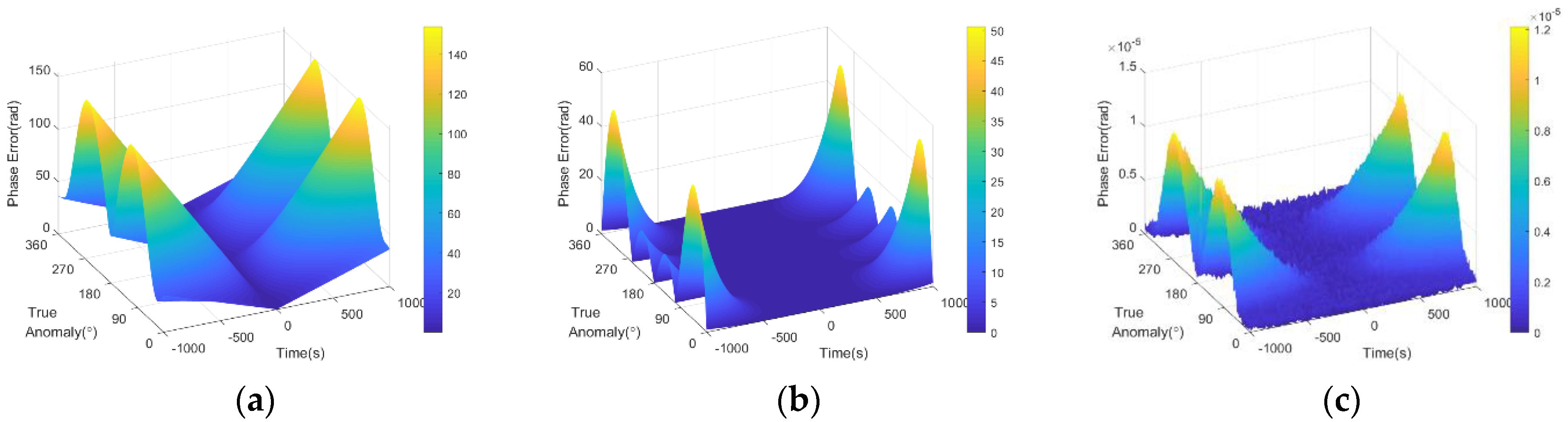
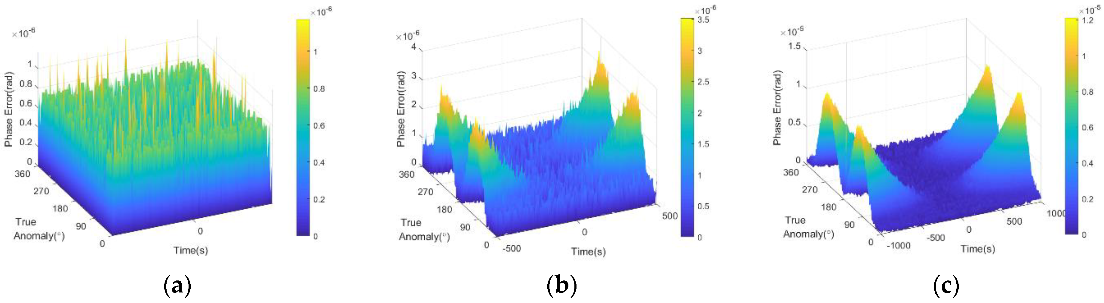
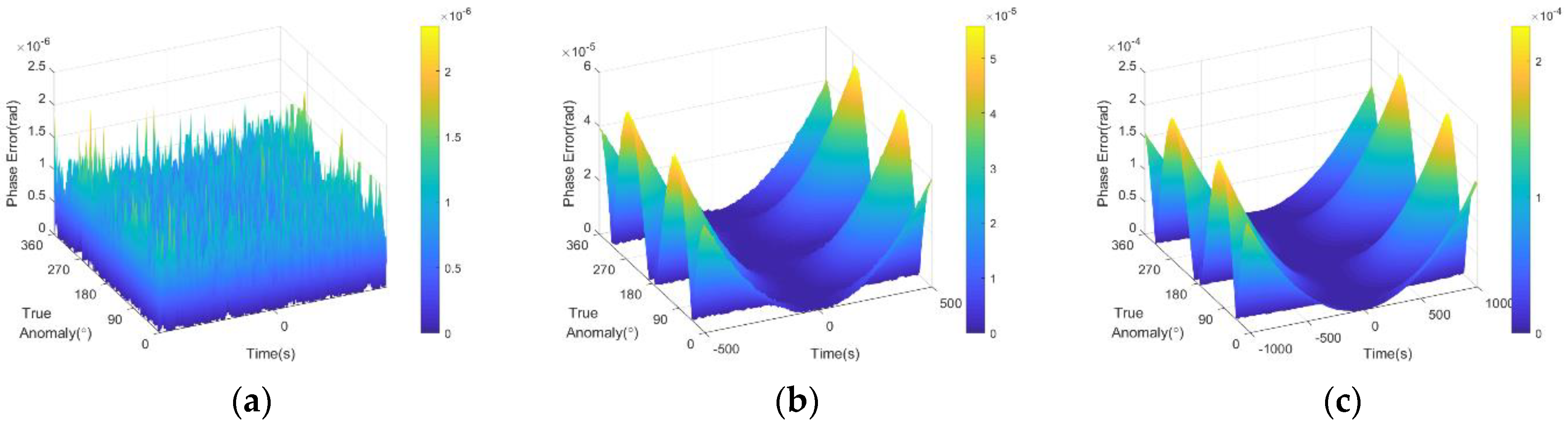
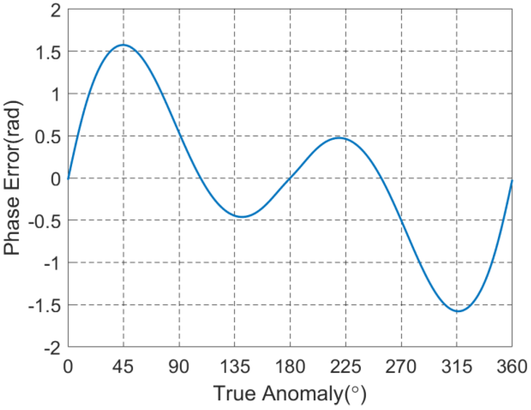
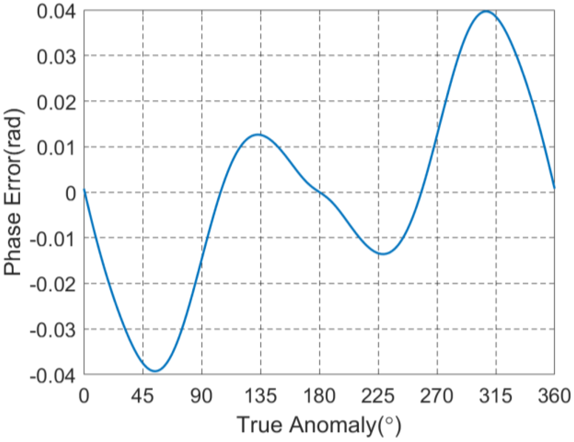
4.2. Fitting Error of Compensation Term

The error of “stop-and-go” assumption mainly comes from replacing the pulse receiving distance with the transmitting distance. However, the equation on the real receiving distance was a transcendental equation and had no analytical solution, so it could only be represented using approximate methods. Considering that the compensation term was derived from iterative approximation and Taylor expansion, its fitting effect would not be better than that of the iterative approximation range model. Figure 12 and Figure 13 show the fitting errors of these two methods for calculating the pulse receiving distance for different integration times. The expansion order used in the proposed method was the same as Equation (33), which is a fifth-order expansion for the first-order term and a first-order expansion for the second-order term.

Comparing Figure 12a and Figure 13a, the fitting error of the proposed compensation term was close to the iterative approximation range model for short integration time. When the observation time increased to 1000 s and 2000 s, the fitting error of the proposed method would be slightly larger than that of the iterative approximation range model. However, the errors were still in the magnitude of 10⁻⁵ and 10⁻⁴ rad, which verified the effectiveness of the proposed compensation term for a long integration time.

According to the above simulation results, it could be seen that the compensation term proposed in this paper had a satisfactory effect for compensating the errors introduced by the “stop-and-go” assumption. Furthermore, considering that the motion of the target was taken into account when deriving the compensation term, it was also applicable to moving targets.

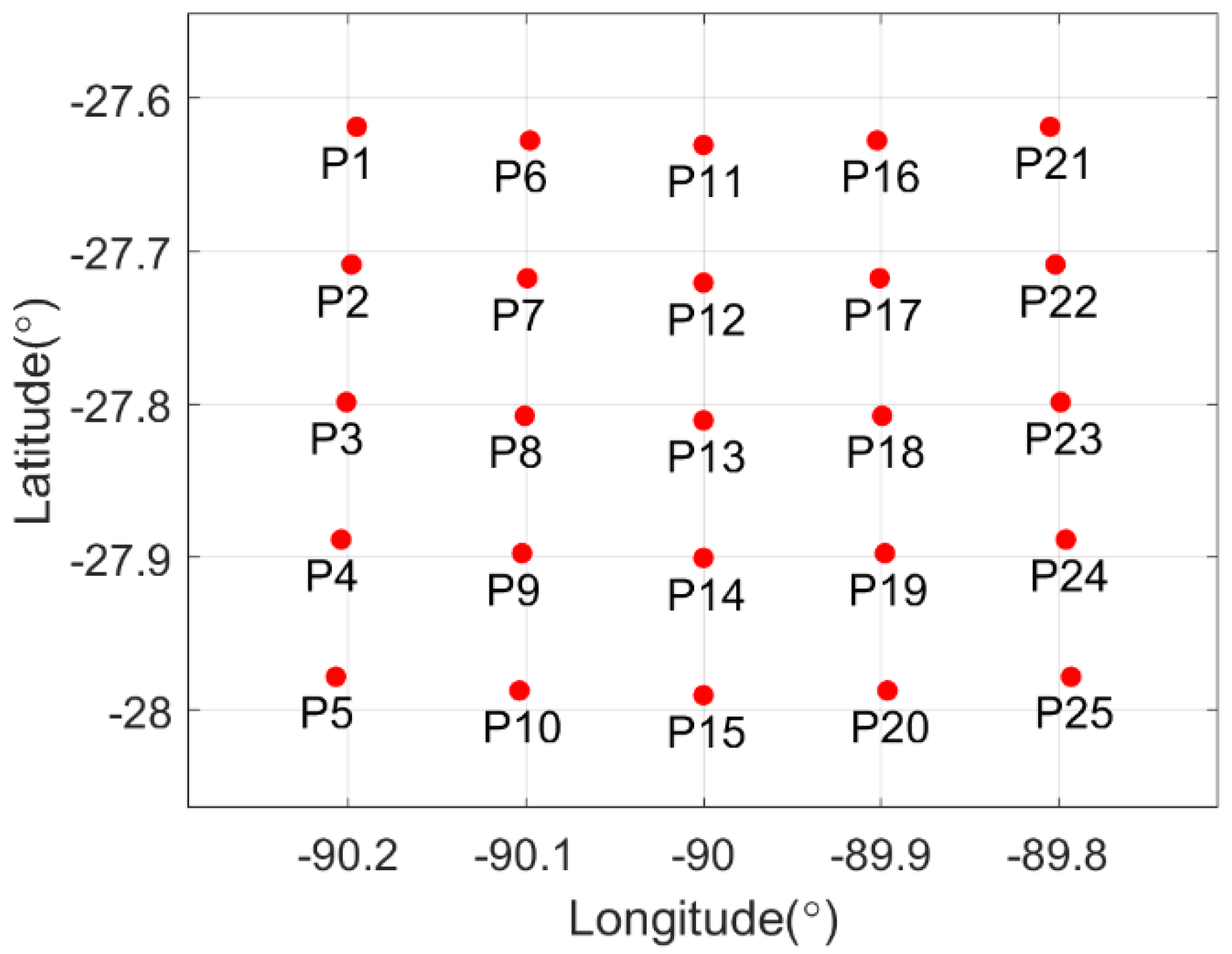
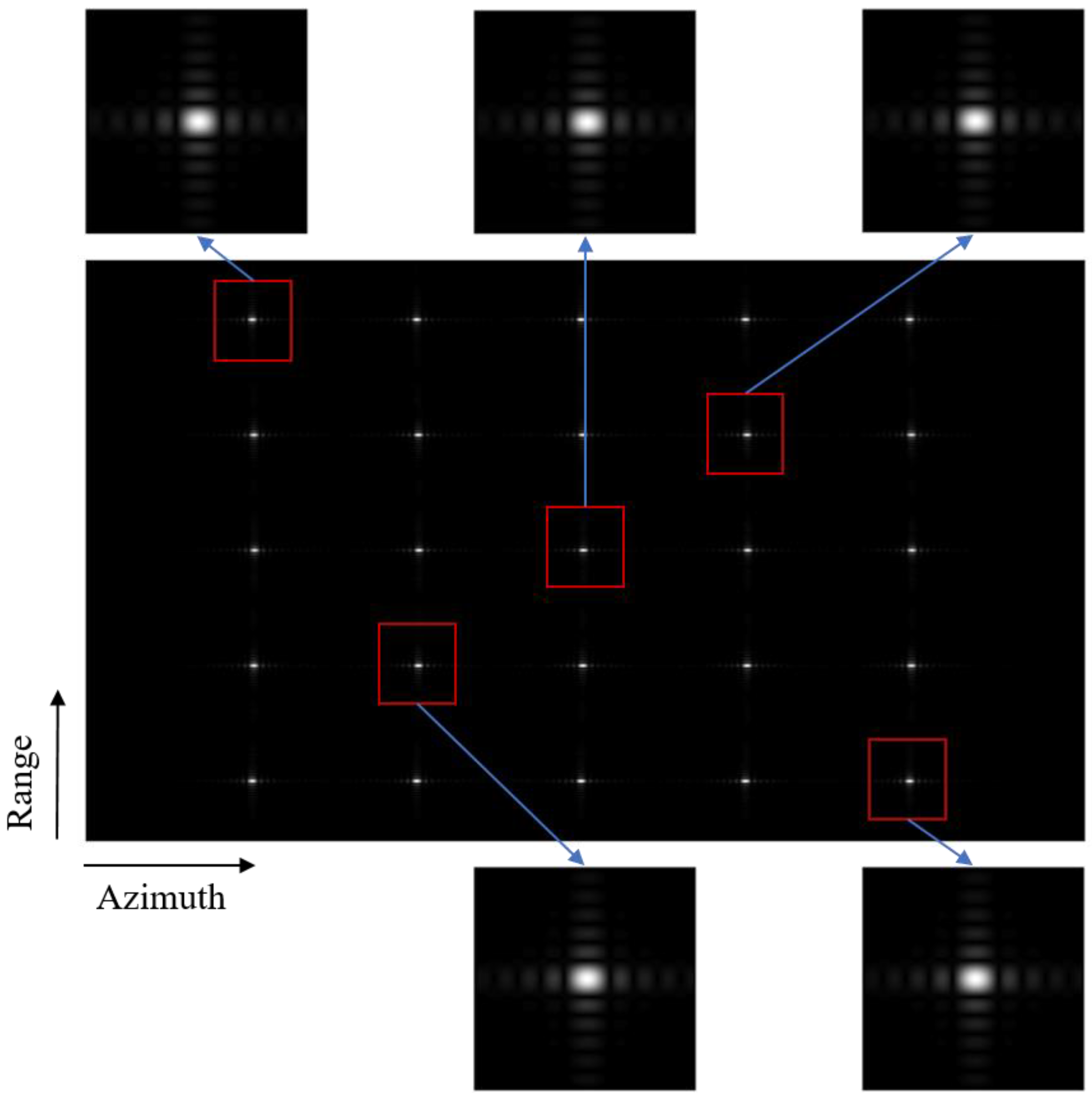
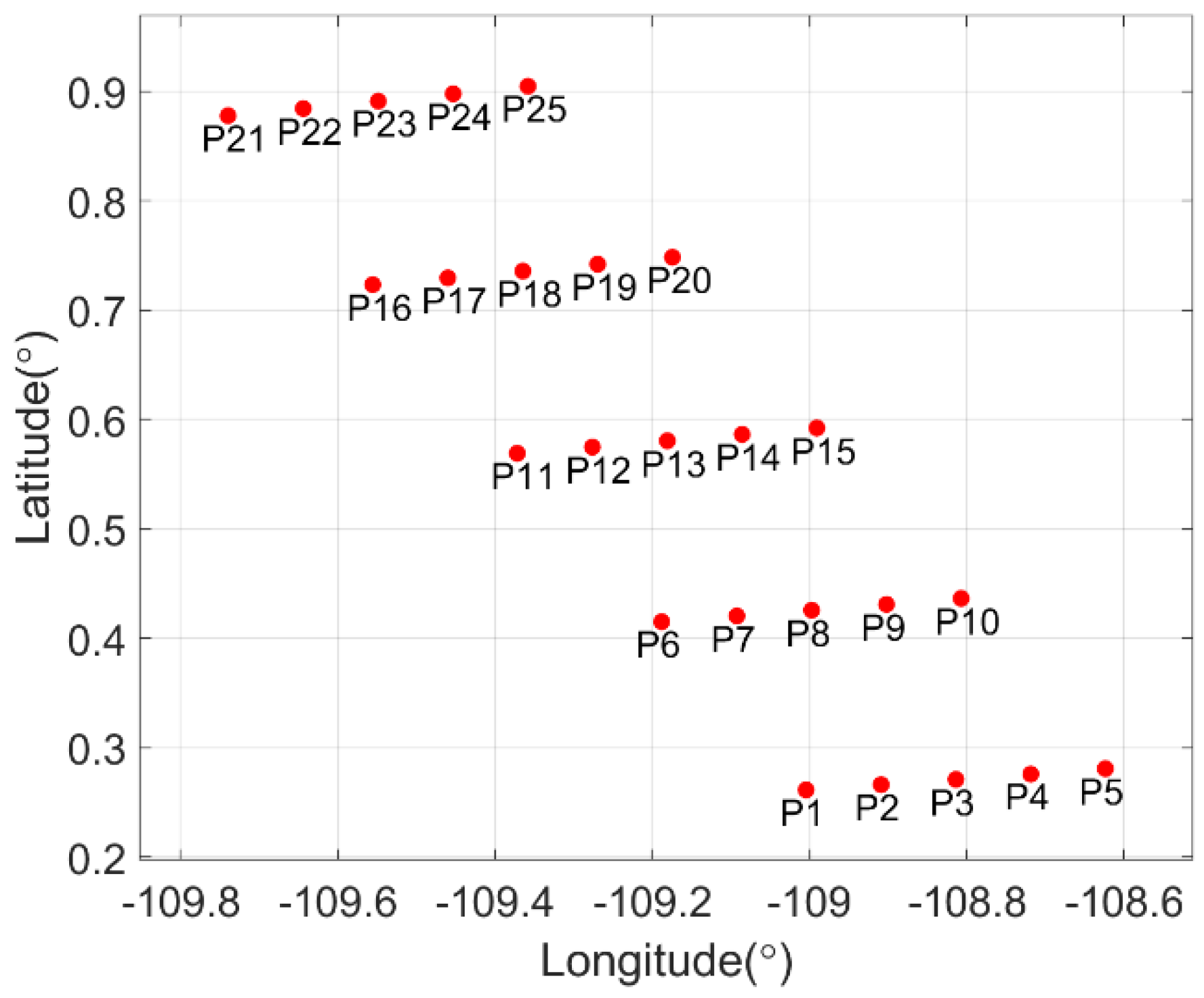
4.3. Focusing Results at Different Orbit Position

Since the motion state of the GEO satellite varied during the flight, the Taylor expansion range model had different fitting effects at different orbit positions. Figure 14 shows the relationship between the fitting error of the fourth-order Taylor expansion and the orbit positions; the observation time was 1000 s.

According to Figure 14, the maximum fitting error of the fourth-order expansion appeared at 45° and 315° of true anomaly, the minimum fitting error appeared in multiple locations, including the perigee and apogee. Therefore, to illustrate the focusing effect at different orbit positions, we conducted the imaging simulations based on fourth-order expansion at perigee and 45° of true anomaly. The simulation parameters are shown in Table 1, and the orbit was chosen as the “8” shaped orbit, the integration time was chosen as 1000 s.

Figure 15 shows the fitting error and the focusing results of the fourth-order Taylor expansion at perigee. From Figure 15a, it can be seen that the fitting error of fourth-order Taylor expansion was much smaller than $\pi /4$, which could lead to a satisfactory focusing results in Figure 15b,c. There were three quality parameters in Figure 15c—impulse response width (IRW), peak sidelobe ratio (PSLR), integrated sidelobe ratio (ISLR). According to the satellite synthetic aperture angle, the theoretical azimuth resolution was 2.2641 m, which was close to the experimental result.

Figure 16 shows the fitting error and focusing result of the fourth-order Taylor expansion at 45° of true anomaly. From Figure 16b,c, it can be seen that the azimuth focusing results of the fourth-order Taylor expansion show obvious asymmetry. The main reason for azimuth-defocusing was that the radial velocity of satellite changed rapidly around this orbit position, and the fourth-order Taylor expansion was difficult to meet the accuracy requirement. According to Figure 16a, the fitting error showed obvious odd function characteristics, which was consistent with the fact that the main term of its reminder was a fifth-order polynomial. The maximum error was about 1.57 rad, which was larger than the error bound $\pi /4$, thus resulting in the defocusing of azimuth.

According to Figure 17a, the fitting error of sixth-order Taylor expansion remained at a very low level at the same position, which could achieve relatively satisfactory focusing results. The imaging results are shown in Figure 17b,c. It should be noted that since the satellite runs faster at this orbit position, this position would obtain a larger synthetic aperture angle and a higher azimuth resolution for the same integration time. The theoretical azimuth resolution was 1.6069 m, which was also close to the experimental result.

Through the above simulation results, it could be seen that since the motion state of satellite changes all the time, the range model of a certain expansion order in different orbit positions would have different fitting effects. The perigee and apogee are always positions with the minimum fitting error, so it is insufficient to verify models or algorithms at only those positions. In conclusion, the expansion order should be determined by the maximum fitting error of the whole orbit, or using different expansion order at different orbit positions for the purpose of reducing the computational burden.

4.4. Focusing Results with Ultralong Integration Time

In order to verify the effectiveness of the mth-order Taylor expansion for target focusing with ultralong integration time, a series of simulation experiments for point targets imaging were conducted. The simulation parameters are shown in Table 1, and the orbit was chosen as the “8” shaped orbit. The integration time was 2000 s in these experiments, and the expansion order of pulse transmitting distance was sixth. Figure 18 shows the relationship between the fitting error of the sixth-order Taylor expansion and orbit position for 2000 s observation time. The imaging positions chosen are 55° of true anomaly and perigee, which were the locations of the maximum and minimum fitting error. The simulation scene was 40 km × 40 km, which had twenty-five point targets established in it, and the intervals between the two adjacent points were both 10 km in the range and azimuth direction. The distribution of point targets in the latitude–longitude grid at perigee is shown in Figure 19.

It needs to be pointed out that these point targets were all placed on the earth surface according to satellite motions and the WGS84 coordinates, rather than being placed on the slant plane, which avoided the problem of targets separated from the earth surface. Targets from P1 to P5 were arranged along the range direction, and the beam scanning velocity was along the longitude at the perigee, according to Figure 19.

The focusing results of twenty-five targets are shown in Figure 20, the horizontal and vertical direction were the azimuth and range directions, respectively. Through the five refined imaging results, the targets located at different positions in the scene could all be well focused.

Table 4. Evaluation parameters of point targets by the imaging method proposed in this paper.

Positions (km)	PSLR(dB)		ISLR(dB)		IRW(m)
	Range	Azimuth	Range	Azimuth	Range	Azimuth
(−20, 20)	−13.29	−13.29	−9.97	−10.54	0.88	1.13
(−10, −10)	−13.29	−13.30	−9.98	−10.54	0.88	1.13
(0, 0)	−13.28	−13.31	−9.97	−10.55	0.88	1.13
(10, 10)	−13.28	−13.32	−9.97	−10.55	0.88	1.13
(20, −20)	−13.30	−13.33	−9.97	−10.56	0.88	1.13

lists the evaluation measures of the five point targets, including PSLR, ISLR, and IRW. The positions in Table 4 indicate the coordinates of the point targets in the imaging scene, and assuming that the center-point was the origin of the coordinates. As shown in Table 4, the range PSLR and azimuth PSLR of different position targets were all close to the theoretical value −13.26 dB, and the ISLR of range direction were also close to the theoretical value −10 dB. It could be seen that the azimuth ISLR were slightly lower than the ideal value, which was mainly because of the curved trajectory of satellite. As for the IRW, the theoretical azimuth resolution of the center-point was 1.1346 m, which was in good agreement with experimental results.

Next, performing the focusing experiment at the true anomaly of 55°. Figure 21 shows the distribution of point targets in the latitude–longitude coordinates. Similar to the previous experiment, the targets from P1 to P5 were arranged along the range direction. However, the difference was that the satellite velocity was no longer parallel to the longitude at this position, so the targets showed an oblique distribution in the latitude–longitude coordinates.

The focusing results and evaluation parameters are shown in Figure 22 and

Table 5. Evaluation parameters of point targets by the imaging method proposed in this paper.

Positions (km)	PSLR(dB)		ISLR(dB)		IRW(m)
	Range	Azimuth	Range	Azimuth	Range	Azimuth
(−20, 20)	−13.30	−13.19	−10.07	−10.55	0.88	0.76
(−10, −10)	−13.29	−13.19	−10.07	−10.57	0.88	0.76
(0, 0)	−13.32	−13.21	−10.07	−10.55	0.88	0.76
(10, 10)	−13.31	−13.20	−10.07	−10.57	0.88	0.76
(20, −20)	−13.31	−13.19	−10.07	−10.56	0.88	0.76

. According to Table 5, most evaluation measures are close to the ideal values. Only the azimuth ISLR was slightly lower than −10 dB, which resulted from the cured trajectory of GEO satellite. The azimuth IRW was 0.76 m at this orbit position, which was close to the theoretical value of 0.7567 m.

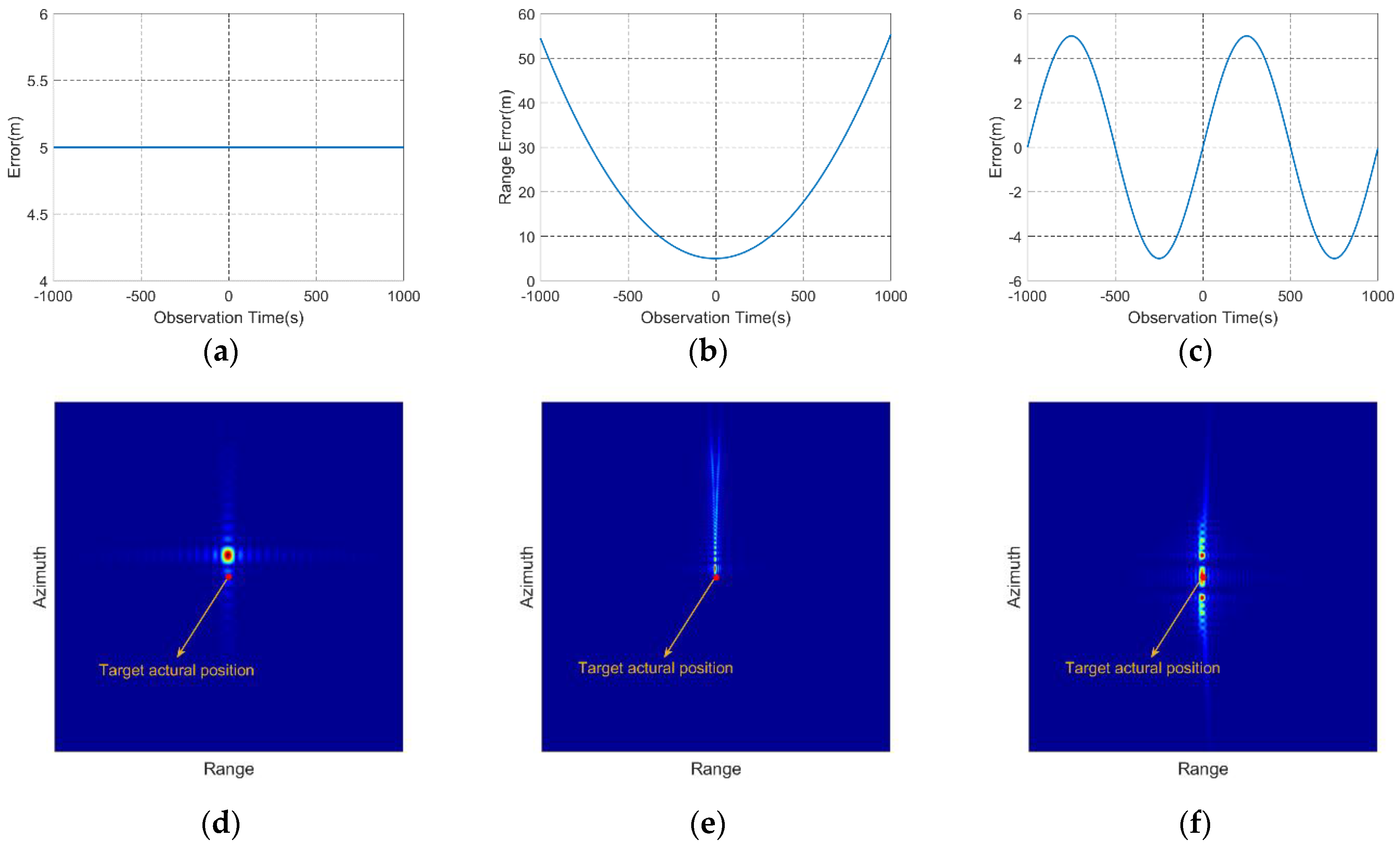
4.5. The Influence of Different Sources of Distortion on Imaging

With an ultralong synthesis time and high resolution in GEO SAR, the sources of distortions in the phase distribution over the antenna synthesis aperture would have many forms. In this section, we briefly discuss the impact of two sources of distortion on imaging:

(1)

Trajectory distortions caused by errors in measuring the parameters of the spacecraft motion.

(2)

Hardware distortions and instabilities during the formation and reception of probing signals (in particular, phase instability, instability of the microwave path parameters).

The simulation parameters are shown in Table 1, and the orbit was chosen as the “8” shaped orbit. The integration time was 2000 s in these experiments, and the orbital position was located at the perigee.

The first was the impact of motion parameter measurement errors. In order to simplify the model, we divided the form of measurement error into common forms such as constant value, quadratic polynomial, and sinusoidal function. The simulation results are shown in Figure 23.

Through the above simulation experiments, it could be seen that the measurement error of satellite motion parameters would cause the target focusing distortion. The form of measurement errors determined the impact on imaging. Constant errors caused the target’s offset, while quadratic polynomial and sinusoidal errors would cause the target to defocus in the azimuth direction.

Next, we discuss the impact of phase errors caused by hardware distortions and instabilities. Similar to the previous experiment, we divided the forms of phase distortion into common forms, such as constant value, quadratic polynomial, and sinusoidal function. The simulation results are shown in Figure 24.

According to Figure 24, the phase error caused by hardware distortions and instabilities also had a certain impact on target focusing. Constant phase errors would not cause obvious changes in the image, while the quadratic polynomial and sinusoidal errors would cause varying degrees of defocus.

As a summary, a slight measurement error and hardware distortion would introduce an intolerant error with the ultralong integration time, which would result in deterioration of the images. Therefore, methods such as calibration and phase autofocus are needed to reduce their influence in the actual system.

5. Conclusions

In view of the wide application prospects, GEO SAR attracts more and more attention from scholars and related organizations. However, the extremely high orbit also brings great challenges to the establishment of accurate slant range models, especially for the range calculation for ultralong time. There are two main difficulties in solving this problem, one is the “stop-and-go” assumption failure caused by the long pulse propagation time, and the other is that the fitting error of traditional low-order Taylor expansion would quickly accumulate at both ends of the aperture.

To solve the problems induced by extremely high orbit and ultralong integration time, an accurate range model based on mth-order Taylor expansion was put forward in this paper. This model was mainly composed of an mth-order Taylor expansion of transmitting distance and an accurate compensation term of the error introduced by the invalidation of “stop-and-go” assumption. The superiority and effectiveness of this new model for ultralong integration time was verified through the simulation experiments. The imaging results demonstrated that this range model was effective for GEO SAR with 2000 s integration time and a 40 km wide imaging scene. The evaluation parameters of point targets were close to the ideal values, and the azimuth resolution could reach 1 meter.

References

1. Cumming, I.; Wong, F. Digital Processing of Synthetic Aperture Radar Data: Algorithms and Implementation; Artech House: Boston, MA, USA, 2005; pp. 113–168. [Google Scholar]
2. Tomiyasu, K. Synthetic aperture radar in geosynchronous orbit. In Proceedings of the 1978 Antennas and Propagation Society International Symposium, Washington, DC, USA, 15–19 March 1978; pp. 42–45. [Google Scholar]
3. Tomiyasu, K.; Pacelli, J. Synthetic aperture radar imaging from an inclined geosynchronous orbit. IEEE Trans. Geosci. Remote Sens. 1983, 21, 324–329. [Google Scholar]
4. Hensley, S.; Chapin, E.; Freedman, A.; Le, C.; Madsen, S.; Michel, T.; Rodriguez, E.; Siqueira, P.; Wheeler, K. First P-band results using the GeoSAR mapping system. In Proceedings of the IEEE 2001 International Geoscience and Remote Sensing Symposium, Sydney, NSW, Australia, 9–13 July 2001; pp. 126–128. [Google Scholar]
5. Madsen, S.; Edelstein, W.; DiDomenico, L.; LaBrecque, J. A geosynchronous synthetic aperture radar; for tectonic mapping, disaster management and measurements of vegetation and soil moisture. In Proceedings of the IEEE 2001 International Geoscience and Remote Sensing Symposium, Sydney, NSW, Australia, 9–13 July 2001; pp. 447–449. [Google Scholar]
6. Madsen, S.; Chen, C.; Edelstein, W. Radar options for global earthquake monitoring. In Proceedings of the IEEE 2002 International Geoscience and Remote Sensing Symposium, Toronto, ON, Canada, 24–28 June 2002; pp. 1483–1485. [Google Scholar]
7. Chen, C.; Raymond, C.; Madsen, S. Observational architectures for enabling earthquake forecasting. In Proceedings of the IEEE 2003 International Geoscience and Remote Sensing Symposium, Toulouse, France, 21–25 July 2003; pp. 618–620. [Google Scholar]
8. NASA JPL. Global Earthquake Satellite System: A 20-Year Plan to Enable Earthquake Prediction; California Institute of Technology: Pasadena, CA, USA, 2003.
9. Hobbs, S. GeoSAR: Summary of the Group Design Project, MSc in Astronautics and Space Engineering 2005/06; College of Aeronautics Rep 509; Cranfield University: Bedford, UK, 2006. [Google Scholar]
10. Hobbs, S.; Bruno, D. Radar imaging from geo: Challenges and applications. In Proceedings of the 2007 Remote Sensing and Photogrammetry Society Annual Conference, Newcastle, UK, 12–14 September 2007; pp. 1–6. [Google Scholar]
11. Bruno, D.; Hobbs, S. Radar Imaging from Geosynchronous Orbit: Temporal Decorrelation Aspects. IEEE Trans. Geosci. Remote Sens. 2010, 48, 2924–2929. [Google Scholar]
12. Hobbs, S.; Sanchez, J.; Kingston, J. Extended lifetime Laplace plane GEO SAR mission design. In Proceedings of the IET International Radar Conference 2015, Hangzhou, China, 14–16 October 2015; pp. 1–4. [Google Scholar]
13. Guarnieri, A.; Rocca, F.; Ibars, A. Impact of atmospheric water vapor on the design of a Ku band geosynchronous SAR system. In Proceedings of the IEEE 2009 International Geoscience and Remote Sensing Symposium, Cape Town, South Africa, 12–17 July 2009; pp. II-945–II-948. [Google Scholar]
14. Guarnieri, A.; Tebaldini, S.; Rocca, F.; Broquetas, A. GEMINI: Geosynchronous SAR for Earth Monitoring by Interferometry and Imaging. In Proceedings of the 2012 IEEE International Geoscience and Remote Sensing Symposium, Munich, Germany, 22–27 July 2012; pp. 210–213. [Google Scholar]
15. Hu, C.; Chen, Z.; Dong, X.; Cui, C. Multistatic Geosynchronous SAR Resolution Analysis and Grating Lobe Suppression Based on Array Spatial Ambiguity Function. IEEE Trans. Geosci. Remote Sens. 2020, 58, 6020–6038. [Google Scholar]
16. Dong, X.; Cui, C.; Li, Y.; Hu, C. Geosynchronous Spaceborne-Airborne Bistatic Moving Target Indication System: Performance Analysis and Configuration Design. Remote Sens. 2020, 12, 1810. [Google Scholar]
17. Xu, W.; Wei, Z.; Huang, P.; Tan, W.; Liu, B.; Gao, Z.; Dong, Y. Azimuth Multichannel Reconstruction for Moving Targets in Geosynchronous Spaceborne–Airborne Bistatic SAR. Remote Sens. 2020, 12, 1703. [Google Scholar]
18. Zhang, Y.; Xiong, W.; Dong, X.; Hu, C. A Novel Azimuth Spectrum Reconstruction and Imaging Method for Moving Targets in Geosynchronous Spaceborne–Airborne Bistatic Multichannel SAR. IEEE Trans. Geosci. Remote Sens. 2020, 58, 5976–5991. [Google Scholar]
19. Li, Y.; Monti Guarnieri, A.; Hu, C.; Rocca, F. Performance and Requirements of GEO SAR Systems in the Presence of Radio Frequency Interferences. Remote Sens. 2018, 10, 82. [Google Scholar]
20. Jiang, M.; Hu, W.; Ding, C.; Liu, G. The Effects of Orbital Perturbation on Geosynchronous Synthetic Aperture Radar Imaging. IEEE Geosci. Remote Sens. Lett. 2015, 12, 1106–1110. [Google Scholar]
21. Li, D.; Zhu, X.; Dong, Z.; Yu, A.; Zhang, Y. Background Tropospheric Delay in Geosynchronous Synthetic Aperture Radar. Remote Sens. 2020, 12, 3081. [Google Scholar]
22. Dong, X.; Hu, J.; Hu, C.; Long, T.; Li, Y.; Tian, Y. Modeling and Quantitative Analysis of Tropospheric Impact on Inclined Geosynchronous SAR Imaging. Remote Sens. 2019, 11, 803. [Google Scholar]
23. Zhang, Y.; Xiong, W.; Dong, X.; Hu, C.; Sun, Y. GRFT-Based Moving Ship Target Detection and Imaging in Geosynchronous SAR. Remote Sens. 2018, 10, 2002. [Google Scholar]
24. Xiong, W.; Zhang, Y.; Dong, X.; Cui, C.; Liu, Z.; Xiong, M. A Novel Ship Imaging Method with Multiple Sinusoidal Functions to Match Rotation Effects in Geosynchronous SAR. Remote Sens. 2020, 12, 2249. [Google Scholar]
25. Zhang, T.; Ding, Z.; Zhang, Q.; Zhao, B.; Zhu, K.; Li, L.; Gao, Y.; Dai, C.; Tang, Z.; Long, T. The First Helicopter Platform-Based Equivalent GEO SAR Experiment with Long Integration Time. IEEE Trans. Geosci. Remote Sens. 2020, 58, 8518–8530. [Google Scholar]
26. Hu, C.; Long, T.; Zeng, T. The accurate focusing and resolution analysis method in geosynchronous SAR. IEEE Trans. Geosci. Remote Sens. 2011, 49, 3548–3563. [Google Scholar]
27. Yu, Z.; Chen, J.; Li, C.; Li, Z.; Zhang, Y. Concepts, properties, and imaging technologies for GEO SAR. In Proceedings of the Sixth International Symposium on Multispectral Image Processing and Pattern Recognition, Yichang, China, 30 October–1 November 2009; Volume 7494, p. 749407. [Google Scholar]
28. Hu, C.; Liu, Z.; Long, T. An improved CS algorithm based on the curved trajectory in geosynchronous SAR. IEEE J. Sel. Top. Appl. Earth Obs. Remote Sens. 2012, 5, 795–808. [Google Scholar]
29. Sun, G.; Xing, M.; Wang, Y.; Yang, J.; Bao, Z. A 2-D Space-Variant Chirp Scaling Algorithm Based on the RCM Equalization and Subband Synthesis to Process Geosynchronous SAR Data. IEEE Trans. Geosci. Remote Sens. 2014, 52, 4868–4880. [Google Scholar]
30. Ding, Z.; Shu, B.; Yin, W. A modified frequency domain algorithm based on optimal azimuth quadratic factor compensation for geosynchronous SAR imaging. IEEE J. Sel. Top. Appl. Earth Obs. Remote Sens. 2016, 9, 1119–1131. [Google Scholar]
31. Hu, C.; Long, T.; Liu, Z.; Zeng, T.; Tian, Y. An Improved Frequency Domain Focusing Method in Geosynchronous SAR. IEEE Trans. Geosci. Remote Sens. 2014, 52, 5514–5528. [Google Scholar]
32. Zhao, B.; Han, Y.; Gao, W.; Luo, Y.; Han, X. A new imaging algorithm for geosynchronous SAR based on the fifth-order Doppler parameters. Prog. Electromagn. Res. B 2013, 55, 195–215. [Google Scholar]
33. Zhao, B.; Qi, X.; Song, H.; Wang, R.; Mo, Y.; Zheng, S. An Accurate Range Model Based on the Fourth-Order Doppler Parameters for Geosynchronous SAR. IEEE Geosci. Remote Sens. Lett. 2014, 11, 205–209. [Google Scholar]
34. Tian, Y.; Yu, W. Accurate slant range model analysis of geosynchronous SAR. J. Electron. Inf. Technol. 2014, 36, 1960–1965. [Google Scholar]
35. Liu, J.; Li, C.; Tan, X.; Shi, P. Characteristics Analysis of “Stop Go Stop” Hypothesis of GEO SAR. Mod. Radar 2014, 36, 38–42. [Google Scholar]
36. Zhang, X.; Huang, P.; Wang, W. Equivalent slant range model for geosynchronous SAR. Electron. Lett. 2015, 51, 783–785. [Google Scholar] [CrossRef]
37. Liu, Q.; Hong, W.; Tan, W. An improved polar format algorithm with performance analysis for geosynchronous circular SAR 2D imaging. Prog. Electromagn. Res. 2011, 119, 155–170. [Google Scholar] [CrossRef] [Green Version]
38. Li, Z.; Li, C.; Yu, Z. Back projection algorithm for high resolution GEO-SAR image formation. In Proceedings of the IEEE 2011 International Geoscience and Remote Sensing Symposium, Vancouver, BC, Canada, 24–29 July 2011. [Google Scholar]
39. Yu, Z.; Zhou, Y.; Chen, J.; Li, C. A new satellite attitude steering approach for zero Doppler centroid. In Proceedings of the IET International Radar Conference, Guilin, China, 20–22 April 2009; pp. 1–4. [Google Scholar]
40. Long, T.; Dong, X.; Hu, C.; Zeng, T. A New Method of Zero-Doppler Centroid Control in GEO SAR. IEEE Geosci. Remote Sens. Lett. 2011, 8, 512–516. [Google Scholar] [CrossRef]
Figure 1. GEO SAR pulse propagation model in the ECEF coordinate system. P is a point target on the earth, S0 is the satellite position when the pulse is transmitted, S1 is the satellite position when the pulse reaches the target, S2 is the satellite position when the pulse is received. r1 and r2 represent the propagation distance of pulse transmission and reception, respectively.
Remotesensing 13 00255 g001
Figure 2. GEO SAR space trajectory. (a) “8” shaped orbit; and (b) near-circular orbit.
Remotesensing 13 00255 g002
Figure 3. GEO SAR velocity. (a) “8” shaped orbit in ECI; (b) “8” shaped orbit in ECEF; (c) Near-circular orbit in ECI; and (d) Near-circular orbit in ECEF.
Remotesensing 13 00255 g003aRemotesensing 13 00255 g003b
Figure 4. GEO SAR integration time. (a) “8” shaped orbit; and (b) near-circular orbit.
Remotesensing 13 00255 g004
Figure 5. Fitting error comparison of several GEO SAR range models. (a) “Stop-and-go” assumption; (b) fourth-order Taylor expansion; and (c) iterative approximation.
Remotesensing 13 00255 g005
Figure 6. The propagation history of the transmitting pulse at the nth PRT. P is a point target on the earth. Rsn, Rtn, Vsn, and Vtn are the position vectors and velocity vectors of satellite and target, respectively.
Remotesensing 13 00255 g006
Figure 7. The Flowchart of the mth-order Taylor expansion process of the pulse transmitting distance in GEO SAR.
Remotesensing 13 00255 g007
Figure 8. The propagation history of transmitting and receiving pulse at the nth PRT. P is a point target on the earth. r1n, r2n represent the transmitting distance vector and receiving distance vector, respectively. τn is the total propagation time of the pulse.
Remotesensing 13 00255 g008
Figure 9. Flowchart of the improved BP algorithm based on the mth-order Taylor expansion range model.
Remotesensing 13 00255 g009
Figure 10. Pulse transmitting distance fitting error comparison of different order Taylor expansion. (a) Fourth-order; (b) fifth-order; and (c) sixth-order.
Remotesensing 13 00255 g010
Figure 11. The maximum phase error of the whole orbit for 6000 s observation time. (a) “8” shaped orbit; and (b) a near-circular orbit.
Remotesensing 13 00255 g011
Figure 12. The fitting error of “stop-and-go” assumption compensation term through the iterative approximation for different integration times. (a) 100 s; (b) 1000 s; (c) 2000 s.
Remotesensing 13 00255 g012
Figure 13. The fitting error of the “stop-and-go” assumption compensation term by the proposed method in this paper for different integration times. (a) 100 s; (b) 1000 s; (c) 2000 s.
Remotesensing 13 00255 g013
Figure 14. The fitting errors of the fourth-order Taylor expansion with 1000 s observation time at different orbit positions.
Remotesensing 13 00255 g014
Figure 15. The fitting error and focusing result of the fourth-order Taylor expansion at perigee. (a) Fitting error; (b) 2-D contour; and (c) azimuth profile.
Remotesensing 13 00255 g015
Figure 16. The fitting error and focusing result of the fourth-order expansion at 45° of true anomaly. (a) Fitting error; (b) 2-D contour; and (c) azimuth profile.
Remotesensing 13 00255 g016
Figure 17. The fitting error and focusing result of sixth-order expansion at 45° of true anomaly. (a) Fitting error; (b) 2-D contour; and (c) azimuth profile.
Remotesensing 13 00255 g017
Figure 18. The fitting errors of the sixth-order Taylor expansion with 2000 s observation time at different orbit positions.
Remotesensing 13 00255 g018
Figure 19. The distribution of twenty-five point targets at perigee.
Remotesensing 13 00255 g019
Figure 20. Focusing results with the range model proposed in this paper for 2000 s integration time at perigee.
Remotesensing 13 00255 g020
Figure 21. The distribution of twenty-five point targets at perigee.
Remotesensing 13 00255 g021
Figure 22. Focusing results with the range model proposed in this paper for 2000 s integration time at 55° of true anomaly.
Remotesensing 13 00255 g022
Figure 23. The simulation results of measurement error. (a) The constant measurement error in the x-axis direction. (b) The quadratic polynomial measurement error in the x-axis direction. (c) The sinusoidal measurement error in the x-axis direction. (d) The imaging result of the constant error. (e) The imaging result of quadratic polynomial error. (f) The imaging result of sinusoidal error.
Remotesensing 13 00255 g023
Figure 24. The simulation results of phase distortion. (a) The constant phase error. (b) The quadratic polynomial phase error. (c) The sinusoidal phase error. (d) The imaging result of constant phase error. (e) The imaging result of quadratic polynomial phase error. (f) The imaging result of sinusoidal phase error.
Remotesensing 13 00255 g024