Characteristics of the Global Radio Frequency Interference in the Protected Portion of L-Band

Abstract

The National Aeronautics and Space Administration’s (NASA’s) Soil Moisture Active–Passive (SMAP) radiometer has been providing geolocated power moments measured within a 24 MHz band in the protected portion of L-band, i.e., 1400–1424 MHz, with 1.2 ms and 1.5 MHz time and frequency resolutions, as its Level 1A data. This paper presents important spectral and temporal properties of the radio frequency interference (RFI) in the protected portion of L-band using SMAP Level 1A data. Maximum and average bandwidth and duration of RFI signals, average RFI-free spectrum availability, and variations in such properties between ascending and descending satellite orbits have been reported across the world. The average bandwidth and duration of individual RFI sources have been found to be usually less than 4.5 MHz and 4.8 ms; and the average RFI-free spectrum is larger than 20 MHz in most regions with exceptions over the Middle East and Central and Eastern Asia. It has also been shown that, the bandwidth and duration of RFI signals can vary as much as 10 MHz and 10 ms, respectively, between ascending and descending orbits over certain locations. Furthermore, to identify frequencies susceptible to RFI contamination in the protected portion of L-band, observed RFI signals have been assigned to individual 1.5 MHz SMAP channels according to their frequencies. It has been demonstrated that, contrary to common perception, the center of the protected portion can be as RFI contaminated as its edges. Finally, there have been no significant correlations noted among different RFI properties such as amplitude, bandwidth, and duration within the 1400–1424 MHz band.

1. Introduction

The protected portion of L-band, i.e., between 1400 and 1427 MHz, has been solely allocated for passive radio astronomy and Earth exploration remote sensing applications [1]. However, significant radio frequency interference (RFI) contamination due to illegal transmitters radiating within this spectrum and out-of-band emissions leaking from adjacent bands has been reported in measurements of L-band microwave radiometers deployed in spaceborne remote sensing missions [2,3]. Such RFI contamination, if not detected and mitigated, may degrade the quality of radiometric data to be used in the retrieval of important geophysical parameters such as soil moisture, sea surface salinity, sea surface wind, and vegetation index; thus, several RFI detection and mitigation algorithms have been developed and implemented in L-band microwave radiometers to address the problem [4]. Pulse blanking techniques in time and frequency domains [5,6], kurtosis and other normality tests [7,8,9,10], polarimetric techniques [11], and spatial domain RFI detection methods [12] are some of these algorithms discussed thoroughly in the literature.

The National Aeronautics and Space Administration’s (NASA) Soil Moisture Active–Passive (SMAP) mission is one of the most recent spaceborne remote sensing missions, which carries a radiometer, operating within the protected portion of L-band, i.e., 1400–1424 MHz, to measure brightness temperatures in horizontal and vertical polarizations from the Earth’s surface to retrieve soil moisture with an acceptable accuracy and uncertainty [13,14]. Unlike previous L-band radiometers, however, the SMAP radiometer includes a digital backend that allows calculating radiometer signal moments in both polarizations as well as their correlations with unprecedented time and frequency resolutions of 1.2 ms and 1.5 MHz, respectively [15].

The signal moments and correlations generated by SMAP’s radiometer digital backend enable a multi-domain comprehensive RFI detection and mitigation procedure, which consists of time domain pulse blanking, cross-frequency detection, kurtosis, and polarimetric RFI detection algorithms. As ground processing, these RFI detection algorithms are simultaneously applied to signal moments and correlations; and, to maximize the probability of RFI detection, flags created by each individual algorithm are combined with a logical “OR” operator. This so-called “maximum probability of detection (MPD)” approach is shown to be capable of detecting and mitigating a significant fraction of the RFI contamination in the protected portion of L-band at the expense of high false-alarm rates [16].

Besides its efficacy to detect and mitigate RFI, SMAP also allows characterization of the RFI environment in the protected portion of L-band in terms of its temporal, spectral, and spatial properties using the geolocated outputs of the SMAP digital backend. These properties determine the performance of RFI detection and mitigation algorithms implemented in microwave radiometry; thus, such characterization is essential for future L-band remote sensing missions. In [17], authors have presented an initial analysis of RFI characteristics in the protected portion of L-band using SMAP’s Level 1A data, i.e., signal moments and correlations produced by its digital backend, which investigated overall RFI bandwidth, duration, and center frequencies for the world as a whole. However, spectrum allocations and usage can be different in different regions and times; thus, further analyses of the RFI properties based on their geographical location and observation times are required. This paper, expanding on a short conference paper presented at the 2019 IEEE International Geoscience and Remote Sensing Symposium [18], addresses this gap in the literature and is structured as follows:

• A short review of SMAP, its radiometer data, and the RFI presence in its radiometer measurements are given in Section 2.
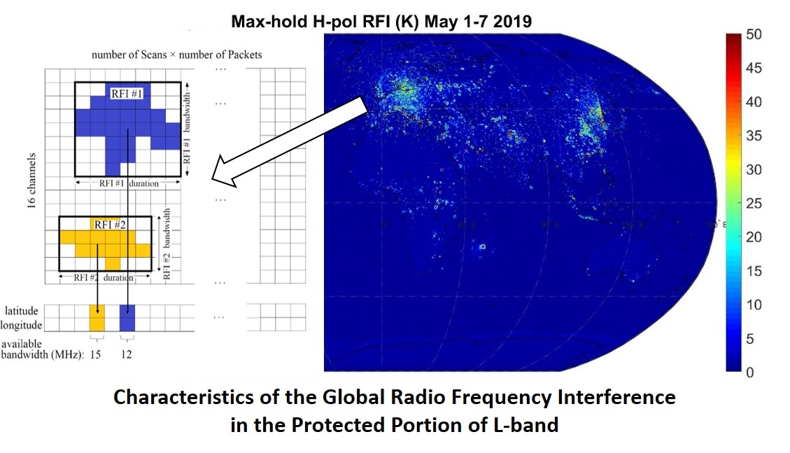
• An RFI detection and characterization procedure, similar to the one discussed in [17,18] with some improvements, applied to SMAP Level 1A data measured between May 1 and 7, 2019 to extract RFI properties in the protected portion of L-band is presented in Section 3. The multi-domain procedure contains time and frequency domain pulse blanking, kurtosis, and skewness algorithms implemented simultaneously. Then, similar to the SMAP data processing, detection results from individual algorithms are combined with a logical “OR” operator.
• Based on detection results, geo-located characteristics of the L-band RFI environment such as the maximum and average RFI bandwidth and duration, average RFI-free bandwidth, and the variance in such properties between ascending and descending SMAP observations are discussed in Section 4. This section also mentions specific frequencies in the protected portion of L-band susceptible to RFI in different geographic regions.
• Finally, Section 5 discusses the results and provides insight for future L-band microwave radiometry missions regarding required RFI detection and mitigation capabilities.

2. SMAP Data and RFI Presence in L-Band

NASA’s Soil Moisture Active–Passive (SMAP) radiometer, owing to its onboard digital backend, provides data from space resolved in both time and frequency within the 1400–1424 MHz spectrum; thus, allowing the retrieval of temporal, spectral, and spatial properties of the RFI environment in the protected portion of L-band. The digital backend produces signal moments and their correlations in full-band, i.e., in a 1 × 24 MHz frequency channel with 300 µs time resolution, and in sub-band, i.e., in 16 × 1.5 MHz frequency channels with 1.2 ms time resolution [15]. These moments in both horizontal and vertical polarizations along with their corresponding geo-location information are stored in publicly available SMAP Level 1A files [19]. The SMAP Level 1B processor first calibrates Level 1A data to obtain brightness temperatures, then implements a multi-domain RFI detection and mitigation procedure that includes time domain pulse blanking (in full-band), cross-frequency detection (in sub-band), kurtosis (in both full-band and sub-band), and polarimetric (in both full-band and sub-band) algorithms. RFI flags of all detectors are combined with logical “OR” operator to maximize the probability of detection, and RFI-free measurements in sub-band are averaged over time and frequency within each radiometer footprint to create RFI-mitigated brightness temperature products [20]. SMAP Level 1B data, also publicly available online [21], contain brightness temperature measurements before and after RFI mitigation, and their differences demonstrate the amplitude of the detected RFI contamination.

Figure 1a,b demonstrates the maximum horizontally polarized (H-pol) brightness temperatures measured by SMAP over 0.25° × 0.25° latitude × longitude grid cells before and after RFI mitigation across the world between May 1 and 7, 2019. It can be seen that, although most of the RFI contamination is successfully removed, some RFI corruption can still be seen even after RFI mitigation. Such persistent RFI, present mostly over Japan and some metropolitan areas in Europe, Middle East and China, is reported to be long-duration and wideband “noise-like” interference, which cannot be easily detected by the SMAP algorithms [22].

Figure 2, on the other hand, shows the maximum RFI amplitude, i.e., the maximum difference between original and RFI-mitigated H-pol brightness temperatures. The figure indicates a significant, worldwide RFI problem for L-band microwave radiometry, which is especially severe over Europe and Eastern Asia. Vertically polarized (V-pol) RFI amplitudes are not shown here but are very similar. It is important to note that brightness temperature values are limited not to exceed 340 K in SMAP Level 1B data, which may result in the underestimation of RFI amplitudes in certain locations with severe contamination. Moreover, since noise-like RFI cannot be properly detected by SMAP, RFI amplitudes where such interference exists are much lower than their true values.

SMAP Level 1B data provide valuable information regarding RFI presence and amplitudes; however, since these brightness temperature products are averaged over radiometer footprints (24 MHz and 9.6 ms), they do not reveal the temporal and spectral properties of the RFI contamination. Thus, in the following sections, SMAP Level 1A data resolved in time and frequency are analyzed to demonstrate these properties.

3. Approach to Reveal L-Band RFI Characteristics

Temporal and spectral properties of L-band RFI can be obtained by applying detection algorithms to publicly available SMAP Level 1A radiometer products. An alternative approach would be analyses of official SMAP RFI flags, resolved in time and frequency, generated by the SMAP Level 1B processor; however, such information is not publicly available. Thus, the RFI detection procedure described in this section and the resulting RFI flags may not be exactly the same as the official SMAP products.

Similar to [17,18], the RFI detection and characterization process of this study starts with preprocessing of the Level 1A data, and then, four different RFI detection algorithms, i.e., cross frequency, time domain pulse blanking, kurtosis, and skewness, are applied to retrieve the properties of RFI observed by SMAP. Note that, unlike SMAP, polarimetry is not used to detect RFI in this study. Below, this process is explained step by step.

3.1. Step I: Statistics Calculations

Kurtosis, skewness, and power (2nd moment) of the sub-band data in each Level 1A file are calculated using the provided signal moments and organized as matrices where rows represent the 16 × 1.5 MHz channels and columns represent 1.2 ms sub-band time packets (the matrices are calculated for in-phase and quadrature components of the radiometer counts separately, then averaged).

3.2. Step II: Cross-Frequency Algorithm

The cross-frequency detection algorithm is applied across the 16 sub-band channels for each 1.2 ms sub-band time packet in the power matrices after the matrices are normalized over the 24 MHz bandwidth using their median values. Then, ith sub-band channel is flagged as RFI contaminated when

$$\left|P_i-P_{median}\right|>3\times MAD$$

(1)

where MAD = median ($\left|P_i-P_{median}\right|$), and $P_i$ and $P_{median}$ denote the power of the ith frequency channel in a 1.2 ms time packet and median power of that packet, respectively. This algorithm is the same as the cross-frequency algorithm presented in [17] but differs from SMAP, which uses mean power and standard deviation instead of median power and median absolute deviation to determine the detection threshold [20]. Use of median and median absolute deviation of power is preferred in this study as the mean and standard deviation values have been found susceptible to bias in the case of RFI presence.

Note that, the cross-frequency algorithm is efficient against RFI signals with limited bandwidths as wideband RFI may distort the median value across the 16 channels and lead to biased thresholds.

3.3. Step III: Time Domain Pulse Blanking Algorithm

The time domain pulse blanking algorithm implements a similar thresholding across 10-SMAP-footprint-long sliding windows for each sub-band channel in the power matrices. In comparison to the time domain thresholding implemented in [17] across 0.4-SMAP-scan-long windows (~96 footprint long), shorter sliding windows are preferred in this study so that biases in coastal regions due to significant brightness temperature differences between aquatic and dry regions can be avoided. RFI flagging is again based on Equation (1), where this time $P_i$ and $P_{median}$ are the ith power sample in a sliding window and the median power of that window, respectively. Note that this algorithm is again different than SMAP as it uses median and median absolute deviation of the measured power instead of its mean and standard deviation.

The time domain algorithm would be efficient in the case of RFI contamination with durations much shorter than the thresholding window used by the algorithm, i.e., 10 SMAP footprints.

3.4. Step IV: Kurtosis Algorithm

The kurtosis detection algorithm flags RFI, in the kurtosis matrices, when a kurtosis sample significantly deviates from the nominal expected RFI-free kurtosis value, which was assumed to be 3 [21]. This procedure can be mathematically formulated as follows:

$$\left|K-3\right|>{\beta }_k{\sigma }_k$$

(2)

where K denotes a measured kurtosis value in the kurtosis matrices; ${\beta }_k$ is the threshold coefficient, which is selected to be 3 in this study; and ${\sigma }_k$ is the standard deviation of the RFI-free kurtosis samples, which can be calculated as described in [17]. This algorithm is the same as the kurtosis algorithm implemented in SMAP [20], and the value of ${\beta }_k$ is selected to set the false alarm rate to 0.3% for this algorithm in RFI-free measurements. ${\beta }_k$ can be decreased if better detection performance is desired at the expense of higher false-alarm rates, or it can be increased if lower false-alarm rates are targeted.

Although the kurtosis algorithm is capable of detecting all non-Gaussian RFI signals, it is reported to be much more sensitive against short-duty-cycle interference [23].

3.5. Step V: Skewness Algorithm

The skewness algorithm performs a thresholding procedure similar to the kurtosis thresholding in the skewness matrices as follows:

$$\left|S-S_{nom}\right|>{\beta }_s{\sigma }_s$$

(3)

where S is a skewness value in the skewness matrices; $S_{nom}$ denotes the expected skewness value for RFI-free measurements, which is assumed to be 0; ${\beta }_s$ is the thresholding coefficient, which again is set to 3; and ${\sigma }_s$ is the standard deviation of RFI-free skewness values which can be calculated as mentioned in [17]. This algorithm, the same as described in [17], is not implemented in SMAP, and the thresholding selection again sets the false-alarm rate to 0.3% in RFI-free cases for the skewness algorithm.

The skewness algorithm searches for asymmetry in the probability distribution function of the radiometer measurements as an indication for RFI contamination [24]. Thus, it is important to note that, since long-duration and constant-amplitude RFI signals that occupy the entire 1.2 ms sub-band time packets shift the overall distribution without spoiling the symmetry, the skewness algorithm is not very efficient against them.

3.6. Step VI: MPD Flags

Similar to what is implemented in SMAP Level 1B processing [20], the outputs, i.e., RFI flags, of the individual detectors described in Steps II–V are combined through a logical “OR” operation as maximum probability of detection (MPD) flags. This procedure increases the false-alarm rate; however, since this study mainly aims to characterize the RFI properties, increased radiometric data loss due to higher false-alarm rates is considered acceptable to obtain the maximum probability of RFI detection.

3.7. Step VII: Identifying Bandwidth and Duration of RFI

To characterize the bandwidth and duration of the L-band RFI contamination, MATLAB built-in functions “bwconncomp” and “regionprops” are used as shown in Figure 3. This approach is previously reported in [17] and implemented in this study without modifications. The “bwconncomp” function combines the neighboring MPD RFI flag samples (eight-connectivity) as single RFI signals occupying multiple time and frequency bins. Then, through the “regionprops” function, the bandwidth and duration of these RFI signals were retrieved. This function, when used with the “BoundingBox” property, measures the dimensions of the smallest rectangle surrounding the RFI signal, and these dimensions correspond to the bandwidth and duration of the RFI signals. However, it is important to acknowledge the fact that this algorithm may unintentionally combine separate RFI sources with overlapping time and frequency bins if they are geographically close; thus, erroneously treat them as single RFI signals.

3.8. Step VIII: Geo-Locating RFI Signals

Finally, RFI signals detected and characterized in previous steps are assigned to their geographical locations based on the latitude and longitude values of their middle points in time. This enables geo-located analyses of the L-band RFI, which has never been reported in detail so far.

4. Results and Discussion

RFI environment observed by the SMAP radiometer in the protected portion of L-band between 1 and 7 May 2019 has been characterized by processing its Level 1A data through the steps listed in the previous section in terms of the bandwidth and duration of RFI signals, availability of RFI-free bandwidth, and the distribution of the RFI contamination in each 1.5 MHz SMAP channel. The following sections discuss these RFI properties based on their geographic location and observation time.

4.1. Spectral Properties of L-Band RFI

Figure 4 illustrates the spectral properties of H-pol RFI contamination observed by SMAP across the world between 1 and 7 May 2019, in terms of maximum and mean bandwidth of RFI signals, average RFI-free spectrum available, and difference in maximum RFI bandwidths between ascending and descending SMAP orbits. V-pol characteristics are not shown here but were found to be very similar.

As seen from the Figure 4a, the maximum RFI bandwidth varies up to 24 MHz, i.e., the entire SMAP band, and wideband RFI mostly appears in Korea, Eastern China, Central Asia, Middle East, and Europe. The average RFI bandwidth, depicted in Figure 4b, on the other hand, usually remains below 4.5 MHz except a few regions such as South Korea, Israel, and Northern England, which indicate continuous and widespread RFI contamination in these locations. The widespread RFI contamination in Northern Europe with maximum and average bandwidths of >10 and ~2.5–3 MHz, respectively, is also noteworthy. Figure 4c shows the average RFI-free spectrum available across the world. The average RFI-free bandwidth over a location, in this study, is defined as follows:

$$avg\left\{SMA{P}_{BW}-{\displaystyle \cup }RF{I}_{BW}\right\}$$

(4)

where $SMA{P}_{BW}$ denotes the entire SMAP bandwidth, i.e., 24 MHz, and $\cup RF{I}_{BW}$ is the bandwidth of the union of all RFI signals observed in that location. As seen from the figure, in general, this parameter seems to be larger than 18 MHz across the world. However, the RFI-free spectrum availability is very limited in some regions such as South Korea, Northern China, Central Asia, and South-Eastern Turkey.

Finally, differences in maximum RFI bandwidths between ascending and descending SMAP orbits may be significant as shown in Figure 4d. Both increases and decreases up to 10 MHz in RFI bandwidth are visible between the ascending and descending measurements in different locations, which is particularly noticeable over Eastern and Central Asia, Europe, and the Middle East. Note that the orange line in the figure that spreads over North-to-South America and indicates large bandwidth differences between ascending and descending orbits is a result of missing descending SMAP measurements over this region between 1 and 7 May 2019.

4.2. Temporal Properties of L-Band RFI

The temporal properties of L-band RFI contamination is described in terms of RFI duration. Figure 5 depicts the maximum and average durations of H-pol RFI signals observed by SMAP across the world between 1 and 7 May 2019, as well as the change in RFI durations between ascending and descending orbits. V-pol characteristics are not shown here but found to be very similar.

As seen from the figure, maximum RFI durations vary substantially based on location; but interference observed longer than 30 ms is not uncommon especially over Europe, the Middle East, and Central and Eastern Asia. These long-duration RFI signals occupy several SMAP footprints (one SMAP footprint is ~9.6 ms); thus, may not be detected efficiently by the SMAP time domain pulse blanking algorithm, which operates within single SMAP footprints.

Average RFI durations, usually below 4.8 ms, seem to be much shorter than the maximum values shown in Figure 5a, indicating spatially and temporally limited RFI contamination. These are also much shorter than duration of a SMAP footprint, which indicates, on average, SMAP time domain pulse blanking algorithms can detect such contamination efficiently. However, there are still a few locations suffering from longer-duration, persistent RFI, i.e., longer than one SMAP footprint, in Central Asia, South-Eastern Turkey, Moscow, and Reunion Island, and it is not surprising that as shown in Figure 1 some of these regions demonstrate RFI signatures even in RFI-free SMAP products. Finally, similar to the extensive wideband RFI corruption in Northern Europe, Northeastern China experiences widespread and relatively long-duration RFI corruption in L-band.

Moreover, similar to bandwidth, RFI durations are also varying considerably with time, between ascending and descending observations. Figure 5c illustrates this (again the large orange line is due to missing data in descending orbits), i.e., the difference in maximum RFI durations between ascending and descending SMAP orbits, which may be significant, up to ~10 ms, which is approximately one SMAP footprint, over Europe, Eastern and Central Asia, the Middle East, and Reunion Island. On the other hand, comparing Figure 4 and Figure 5, one can conclude that the change in the temporal and spectral properties of the L-band RFI environment between ascending and descending measurements is not necessarily correlated. Moscow and Reunion Island, where only RFI durations change between ascending and descending observations, are examples of this observation.

4.3. Spectral Distribution of L-Band RFI

Previous microwave radiometers operating in L-band such as Soil Moisture and Ocean Salinity (SMOS) [25,26,27,28] and Aquarius [29,30] have only one frequency channel occupying the protected portion of L-band; thus, it has not been possible to determine which frequencies within this spectrum are susceptible to RFI contamination. Due to its 16 × 1.5 MHz frequency channels, on the other hand, SMAP has enabled such analyses. This study defines the RFI percentage in a SMAP channel, $\%RF{I}_{ch}$, as follows:

$$\%RF{I}_{ch}=\frac{C{h}_{flag}}{T_{flag}}\times 100$$

(5)

where $C{h}_{flag}$ denotes the number of MPD RFI flags within that SMAP channel and $T_{flag}$ is the number total MPD RFI flags in all 16 frequency channels. For instance, if RFI exists only in one SMAP channel over a region, $\%RF{I}_{ch}$ is 100 for that channel and 0 for all other channels over that area. On the other hand, if RFI contamination is equally distributed in all SMAP channels, then, $\%RF{I}_{ch}$ is 6.25% for all channels. Figure 6 and Figure 7 show H-pol $\%RF{I}_{ch}$ for all SMAP frequency channels across the world (V-pol results are not shown here but found to be similar). These figures indicate that, contrary to popular belief, RFI contamination is not necessarily concentrated at the edges of the protected portion of L-band due to leakage from adjacent bands, as some strong RFI sources can be observed in 1409, 1410.5, 1412, 1413.5, and 1415 MHz channels. Over Northern Europe and Reunion Island, for example, $\%RF{I}_{ch}$ at these frequencies varies between 12 and 20. On the other hand, at the edges of the SMAP band, i.e., 1400/1424, 1401.5, and 1403 MHz, as well as 1421, and 1422.5 MHz, severe RFI contamination exists and $\%RF{I}_{ch}$ ranges from 10 to more than 20 over Central and Eastern Asia, Eastern Europe, North-Eastern Africa, and, especially in 1400/1424 and 1401.5 MHz channels, over Italy. Considering the overall worldwide RFI distribution across the SMAP channels given in [17], it is still expected that sum of RFI contamination within these channels constitutes the majority of L-band RFI.

4.4. Overall Worldwide Spectro-Temporal RFI Properties

Besides separate analyses of temporal and spectral properties of L-band RFI and their geographical distribution, a worldwide and cumulative joint analysis of these features is useful. Figure 8 shows the average RFI duration versus average RFI bandwidth observed by SMAP in horizontal polarization during its ascending and descending orbits between 1 and 7 May 2019 (V-pol results are not shown here but found to be similar). As seen from the figure, the average L-band RFI is mostly short (<9.6 ms) and narrowband (<5 MHz); however, significant number of cases with longer durations or wider bandwidths have also been observed. RFI signals with both long durations and wide bandwidths are particularly of interest to the microwave radiometry community as such noise-like interference cannot be easily detected by the traditional algorithms listed in Section 3. Another notable information Figure 8 presents is that, although a small correlation can be seen between RFI bandwidth and minimum RFI duration, i.e., the minimum RFI duration observed for a certain bandwidth increases with bandwidth itself, observed RFI durations and bandwidths are predominantly uncorrelated.

5. Conclusions and Discussion

This paper presents the geo-located temporal and spectral characteristics of RFI present in the protected portion of L-band. It has been shown that bandwidth, duration, and spectral distribution of L-band RFI may vary significantly with location and observation time, and there is no strong correlation between these features.

Table 1. L-band RFI properties over different continents.

RFI Properties	Africa	Asia	Europe	Americas	Oceania
Amplitude	>50 K RFI over Reunion Island. Strong RFI, >50 K, over Sudan, South Sudan, DRC, Nigeria, and Algeria.	>50 K RFI mostly concentrated over discrete regions over Central Asia, the Middle East, and South-Eastern Asia. Widespread, >20K, RFI contamination over Eastern China.	Widespread, >20 K, RFI contamination over Northern Europe. Several discrete regions with >50 K RFI over Southern Europe.	Discrete >50 K RFI regions over Colombia and Cuba. Discrete locations in the U.S. and Brazil with 20–50 K RFI.	~15–20 K RFI near Melbourne.
Average Bandwidth	Discrete regions over Eastern Tanzania and Central African Rep. with >4.5 MHz bandwidth.	Wideband RFI over South Korea, Taipei, and Israel with >4.5 MHz bandwidth. 3–4.5 MHz bandwidth over Eastern China, Central Asia, and the Middle East.	Wideband RFI over UK and continental Europe with >4.5 MHz bandwidth. Widespread RFI over Northern Poland and Germany with 2.5–3.5 MHz bandwidth.	A few discrete locations in South America and Alaska with RFI bandwidth >4.5 MHz RFI.	RFI over Northern Australia with 2.5–3 MHz bandwidth.
Maximum Bandwidth	Discrete regions in Central Africa with RFI bandwidth up to 24 MHz.	RFI with up to 24 MHz bandwidth over Eastern China, South Korea, Central Asia, and the Middle East.	Several regions all over the continent with RFI bandwidth up to 24 MHz.	Regions in South America, Mexico, and Central U.S. with RFI bandwidth up to 24 MHz.	RFI with 24 MHz bandwidth over two locations in Northern Australia.
Average RFI-free Bandwidth	>20 MHz except few regions in Sudan, South Sudan, and DRC. <12 MHz over Reunion Island and regions in Eastern Tanzania and DRC.	>20 MHz except Eastern China, Central Asia, and the Middle East. Regions in South Korea, Northern China, and South-Eastern Turkey suffer from limited, <12 MHz, band availability.	Mostly >18 MHz all over the continent.	Mostly >20 MHz with discrete regions having 1–2 MHz-less RFI-free spectrum.	Mostly >20 MHz.
Difference in Maximum Bandwidth between Ascending and Descending Orbits	Ascending bandwidths are larger up to 10 MHz over discrete regions in Central Africa.	>10 MHz wider bandwidth in ascending then descending over Eastern China and Central Asia. ~10 MHz wider bandwidth in descending orbits over discrete locations in China, Northern India, and the Middle East	Descending bandwidths are usually 5–10 MHz larger in Central and Eastern Europe. Over the Balkans and Italy, discrete regions with ~10 MHz larger ascending bandwidths.	~10 MHz wider bandwidths in ascending orbits over certain locations Central and Southern U.S as well as Mexico.	No difference observed.
Average Duration	>4.5 ms over certain locations in Reunion Island, DRC, Sudan, South Sudan, and Algeria.	>4.5 ms over certain locations in South Korea, Central Asia, and the Middle East. Widespread RFI with ~2.5 ms duration over Northern China.	>4.5 ms over Moscow, Russia, and discrete locations in Southern Europe.	>4.5 ms over a location in Colombia.	RFI near Melbourne with ~2.5–3.5 ms duration.
Maximum Duration	>80 ms over locations in Reunion Island, Sudan, Nigeria, Algeria, and DRC.	>90 ms over locations in South Korea, Central Asia, and the Middle East. Widespread RFI with durations 30–50 ms.	>90 ms over locations in Central Russia, the Balkans, and Italy. Many more locations with 30–50 ms durations all over the continent.	>90 ms over a few locations in Colombia, Chile, and Argentina. 30–50 ms RFI over regions in Eastern U.S., California, and Brazil.	30–50 ms over discrete regions in South-Eastern Australia.
Difference in RFI Duration between Ascending and Descending Orbits	>8 ms difference over locations in Reunion Island, Algeria, Nigeria, Sudan, DRC, Uganda, and Kenya.	>8 ms difference over several regions in Eastern China, South Korea, Central and South-Eastern Asia, and the Middle East.	Widespread difference up to >8 ms all over the continent.	Discrete locations in North and South America with differences up to >8 ms.	No significant differences observed.

summarizes the overall results of this study regarding the temporal and spectral properties of L-band RFI as well as the amplitude information extracted from SMAP Level 1A and 1B data for each continent.

Table 2. RFI percentages ($\%RF{I}_{ch}$) in SMAP channels over different continents.

SMAP Channels	Africa	Asia	Europe	Americas	Oceania
1400/1424 MHz	>20 over certain regions in Sudan, South Sudan, Ethiopia, and Uganda.	>20 over regions in Central Asia, South-Eastern China, and the Middle East. ~10 over many other locations in Eastern China and the Middle East.	>20 over many regions in Italy, the Balkans, and Northern Spain. Widespread RFI with RFI percentage ~10 over Eastern Europe and Russia.	>20 over discrete regions in Colombia, Chile, and California.	No significant RFI observed.
1401.5 MHz	>20 over certain regions in South Sudan and Uganda.	>20 over a few regions in Northern India and Eastern China. ~10 over several locations in the Middle East and Central Asia.	>20 over many regions in Italy, Ukraine, Russia, and the tU.K. Several locations with RFI percentage ~10 over Eastern Europe and Russia.	>20 over discrete regions in Mexico, Chile, and California.	No significant RFI observed.
1403 MHz	>20 over locations in Algeria and Rwanda/Burundi.	>20 over regions in Central Asia, Turkey, and Eastern China. Widespread RFI with RFI percentage ~10 over Central Asia.	>20 over Albania and many locations in Russia. ~10 over several locations across the continent.	>20 over certain locations in Texas and California. ~12 over regions in Mexico and Chile.	No significant RFI observed.
1404.5 MHz	>20 over locations in Algeria.	>20 over Southern Saudi Arabia and Northern Yemen. 8–15 over several regions in Central Asia, India, and Turkey.	15–20 over several locations in Russia and Ukraine.	No significant RFI observed.	No significant RFI observed.
1406 MHz	~15 over a coastal region near Ghana.	>20 over certain locations in the Philippines and Pakistan. Widespread RFI with RFI percentage 8–16 over China and Korea.	8–20 over discrete regions in Russia and the Balkans.	>20 over a region in Ecuador.	No significant RFI observed.
1407.5 MHz	12–20 over several locations in Ghana, Uganda, Rwanda/Burundi, and Congo.	>20 over many regions in Central Asia. 12–15 over several locations in China and Korea. ~12 over Sinai and Tajikistan.	>20 over regions in Southern Italy and Central Russia. 8–12 over many regions throughout the continent.	No significant RFI observed.	No significant RFI observed.
1409 MHz	>20 over locations in Nigeria, Uganda and Congo. 10–15 over regions in Rwanda/Burundi and Ghana.	>20 over several locations in Central Asia, Korea, and the United Arab Emirates. 8–12 over several locations in China, Korea, and Sinai.	>20 over a few regions in Northern Italy, Southern France, and Spain. 8–14 over several locations in Russia and continental Europe.	~20 over some locations in Brazil, Argentina, Cuba, and California.	No significant RFI observed.
1410.5 MHz	>20 over locations in Libya, Nigeria, Uganda, and Congo. 10–14 over some locations in Ghana and Rwanda/Burundi.	>20 over regions in Bangladesh, Pakistan, Hong Kong, and Taiwan. 8–14 over several location in Central Asia, China, Korea, and Sinai.	>20 over a few regions in Northern Italy, Southern France, and near Moscow. Widespread RFI with RFI percentage 10–12 over Northern and Central Europe.	~20 over some locations in Argentina.	No significant RFI observed.
1412 MHz	>20 over regions near Congo and Libya. ~12 over a location near Ghana.	>20 over several locations in Kuwait, Central Asia, Bangladesh, North-Eastern China, Caucasus, and Siberia. 8–12 over a large region in Pakistan and Afghanistan.	Widespread RFI over almost the entire continent with >8 RFI percentage. >20 over discrete regions in Russia.	15–20 over a few regions in Argentina and Brazil.	No significant RFI observed.
1413.5 MHz	Widespread RFI with RFI percentage >20 over Reunion Island. >20 over a location near Congo.	>20 over a few locations in Bangladesh, Central Asia, and Northern China. 8–12 over a few regions in Pakistan, China, and Korea.	Widespread RFI over almost the entire continent with >8 RFI percentage. >20 over discrete regions in Russia, Germany, and Sweden.	>20 over a few locations in Brazil.	No significant RFI observed.
1415 MHz	>20 over locations near Congo and Reunion Island.	~14 over certain regions in Saudi Arabia, Pakistan, and Bangladesh. 8–12 over several locations in the Middle East, Pakistan, China, and Korea.	Widespread RFI with RFI percentage 10–12 over Northern Europe. ~15 over several locations in Portugal, Russia, and Central Europe.	15–20 over several locations in New England, Chicago as well as in Argentina, Mexico, Peru, and Ecuador.	No significant RFI observed.
1416.5 MHz	10–12 over a few regions near Congo and Central African Republic.	8–20 over many regions in China, Korea, Central Asia, Iran, Saudi Arabia, and Siberia.	8–20 over several regions throughout the continent.	No significant RFI observed.	No significant RFI observed.
1418 MHz	Large RFI with RFI percentage >20 over Algeria. 10–12 over some regions in Central Africa.	>20 over regions in Pakistan, Taiwan, Central Asia, Turkey, and Northern Japan. 8–14 over several regions in the Middle East, Siberia, China, and Central Asia.	>10 over many regions in Central and Eastern Europe, Greece, Southern Italy, Spain, and Portugal.	>20 over a few regions in New England, Northern U.S., and Canada.	>15 over a few discrete regions in Southern and Eastern Australia.
1419.5 MHz	10–14 over a few locations in Central Africa and South Sudan.	>12 over many regions in Turkey, the Middle East, Pakistan, Central Asia, and Siberia.	>8 over several discrete regions scattered over the continent.	No significant RFI observed.	~15 over a region in Eastern Australia.
1421 MHz	>20 over a few regions in Sudan, South Sudan, and near Libya. ~10 over a few regions in Central and Eastern Africa.	10–16 over several regions in China, the Middle East, Central Asia, and Siberia.	>8 over several discrete regions scattered over the continent.	>12 over discrete regions in Cuba as well as Northern and Eastern U.S.	No significant RFI observed.
1422.5 MHz	>20 over a few locations in Libya, Sudan, and South Sudan.	12–14 over many locations in the Middle East. ~20 over several regions in Myanmar, Bangladesh, and China. ~8–10 over scattered discrete regions.	>20 over a large area in the Balkans. >20 over discrete regions over Spain and Northern Europe. Widespread RFI over Eastern Europe with RFI percentage 8–10.	>14 over a region near the Great Lakes.	No significant RFI observed.

, on the other hand, demonstrates the RFI contamination in each SMAP frequency channel to specify particular frequencies, which are not necessarily at the edges of the protected portion of L-band, susceptible to RFI over different locations.

The results of this study, indicating that temporal and spectral properties of L-band RFI may vary considerably with time and location, suggest that multi-domain comprehensive RFI detection algorithms supported by advanced digital backends, as implemented in SMAP, are good steps toward identifying and removing interference in radiometric measurements. On the other hand, to decrease false-alarm rates and data loss, dynamic weights and thresholds should be introduced to such algorithms, which can adjust the entire RFI detection and mitigation procedure based on time and location of the measurements. Machine learning and artificial intelligence methods, which are becoming popular recently in remote sensing applications [31,32,33], can be used to train radiometers as these instruments orbit the Earth to tune the RFI detection parameters in real time.

Finally, one should note that the performance of RFI detection and characterization algorithms applied in this study, and thus the durations and bandwidths presented in this paper, are constrained by SMAP’s 1.2 ms temporal, 1.5 MHz spectral, and ~40 km spatial resolutions. More capable radiometers in future spaceborne remote sensing missions with higher data sampling rates and spatial resolutions would reveal more accurate information regarding the L-band RFI characteristics. In addition, due to the substantial size of SMAP Level 1A data files, only one week of SMAP measurements were analyzed. RFI properties are known to change in time; but, although different time periods may demonstrate different characteristics, this one week was found to be enough to present the main conclusions of this study summarized in the previous paragraphs, i.e., (1) bandwidth, duration, and spectral distribution of L-band RFI may vary significantly with location and observation time, (2) RFI contamination is not limited to the edges of the protected portion of L-band, and (3) multi-domain comprehensive detection algorithms with dynamic weights and thresholds are required for proper RFI mitigation. Finally, the detection procedure described in Section 3 is not very efficient against wideband and long-duration, i.e., noise-like, RFI contamination. For instance, over Japan, no L-band RFI was detected in this study although the region is known to be heavily RFI contaminated in L-band [34]. As more effective algorithms are developed against such noise-like RFI, they can be included in future studies to characterize the L-band RFI environment more precisely.

References

1. National Research Council. Handbook of Frequency Allocations and Spectrum Protection for Scientific Uses; The National Academies Press: Washington, DC, USA, 2007.
2. Aksoy, M.; Johnson, J.T. A Comparative Analysis of Low-Level Radio Frequency Interference in SMOS and Aquarius Microwave Radiometer Measurements. IEEE Trans. Geosci. Remote Sens. 2013, 51, 4983–4992. [Google Scholar] [CrossRef]
3. Aksoy, M.; Johnson, J.T. A Study of SMOS RFI Over North America. IEEE Geosci. Remote Sens. Lett. 2013, 10, 515–519. [Google Scholar] [CrossRef]
4. Lahtinen, J.; Uusitalo, J.; Ruokokoski, T.; Ruoskanen, J. Evaluation and comparison of RFI detection algorithms. In Proceedings of the 2016 14th Specialist Meeting on Microwave Radiometry and Remote Sensing of the Environment (MicroRad), Espoo, Finland, 11–14 April 2016; pp. 62–67. [Google Scholar]
5. Niamsuwan, N.; Johnson, J.T.; Ellingson, S.W. Examination of a simple pulse-blanking technique for radio frequency interference mitigation. Radio Sci. 2005, 40, 1–11. [Google Scholar] [CrossRef] [Green Version]
6. Güner, B.; Johnson, J.T.; Majurec, N. Performance analysis of a cross-frequency detector of pulsed sinusoidal RFI in Mi-crowave Radiometry. In Proceedings of the 2009 IEEE International Geoscience and Remote Sensing Symposium, Cape Town, South Africa, 12–17 July 2009. [Google Scholar]
7. Tarongi, J.M.; Camps, A. Normality Analysis for RFI Detection in Microwave Radiometry. Remote Sens. 2009, 2, 191–210. [Google Scholar] [CrossRef] [Green Version]
8. Güner, B.; Frankford, M.T.; Johnson, J.T. A Study of the Shapiro–Wilk Test for the Detection of Pulsed Sinusoidal Radio Frequency Interference. IEEE Trans. Geosci. Remote Sens. 2009, 47, 1745–1751. [Google Scholar] [CrossRef]
9. Bradley, D.; Morris, J.M.; Adali, T.; Johnson, J.T.; Aksoy, M. On the detection of RFI using the complex signal kurtosis in microwave radiometry. In Proceedings of the 2014 13th Specialist Meeting on Microwave Radiometry and Remote Sensing of the Environment (MicroRad), Pasadena, CA, USA, 24–27 March 2014; pp. 33–38. [Google Scholar]
10. De Roo, R.D. A Simplified Calculation of the Kurtosis for RFI Detection. In Proceedings of the IGARSS 2008–2008 IEEE International Geoscience and Remote Sensing Symposium, Boston, MA, USA, 9 October 2008; pp. 3755–3760. [Google Scholar]
11. Kristensen, S.S.; Balling, J.; Skou, N.; Sobjoerg, S.S. RFI in SMOS data detected by polarimetry. In Proceedings of the 2012 IEEE International Geoscience and Remote Sensing Symposium, Munich, Germany, 22–27 July 2012; pp. 3320–3323. [Google Scholar]
12. Soldo, Y.; Le Vine, D.M.; Bringer, A.; Mohammed, P.N.; De Matthaeis, P.; Piepmeier, J.R.; Johnson, J.T. Recent Advances in SMAP RFI Processing. In Proceedings of the IGARSS 2018–2018 IEEE International Geoscience and Remote Sensing Symposium, Valencia, Spain, 22–27 July 2018; pp. 313–315. [Google Scholar]
13. Entekhabi, D.; Njoku, E.; O’Neill, P.; Spencer, M.; Jackson, T.; Entin, J.; Im, E.; Kellogg, K. The soil moisture active/passive mission (SMAP). In Proceedings of the IGARSS 2008–2008 IEEE International Geoscience and Remote Sensing Symposium, Boston, MA, USA, 7–11 July 2008. [Google Scholar]
14. Entekhabi, D.; Njoku, E.; O’Neill, P. The soil moisture active and passive mission (SMAP): Science and applications. In Proceedings of the 2009 IEEE Radar Conference, Pasadena, CA, USA, 4–8 May 2009; pp. 1–3. [Google Scholar]
15. Piepmeier, J.R.; Johnson, J.T.; Mohammed, P.N.; Bradley, D.; Ruf, C.; Aksoy, M.; Garcia, R.; Hudson, D.; Miles, L.; Wong, M. Radio-Frequency Interference Mitigation for the Soil Moisture Active Passive Microwave Radiometer. IEEE Trans. Geosci. Remote Sens. 2014, 52, 761–775. [Google Scholar] [CrossRef]
16. Mohammed, P.N.; Aksoy, M.; Piepmeier, J.R.; Johnson, J.T.; Bringer, A. SMAP L-Band Microwave Radiometer: RFI Miti-gation Prelaunch Analysis and First Year On-Orbit Observations. IEEE Trans. Geosci. Remote Sens. 2016, 54, 6035–6047. [Google Scholar] [CrossRef]
17. Rajabi, H.; Aksoy, M. Characteristics of the L-Band Radio Frequency Interference Environment Based on SMAP Radiom-eter Observations. IEEE Geosci. Remote Sens. Lett. 2019, 16, 1736–1740. [Google Scholar] [CrossRef]
18. Aksoy, M.; Rajabi, H. Characteristics of radio frequency interference in the protected portion of L-Band. In Proceedings of the IGARSS 2019–2019 IEEE International Geoscience and Remote Sensing Symposium, Yokohama, Japan, 28 July–2 August 2019; pp. 4539–4542. [Google Scholar]
19. SMAP L1A Radiometer Time-Ordered Parsed Telemetry, Version 2. National Snow and Ice Data Center. 2019. Available online: https://nsidc.org/data/SPL1AP/versions/2 (accessed on 1 June 2019).
20. Piepmeier, J. SPL1AP/BTB Algorithm Theoretical Basis Document Version 2; NASA: Washington, DC, USA, 2016. [Google Scholar]
21. SMAP L1B Radiometer Half-Orbit Time-Ordered Brightness Temperatures, Version 4\National Snow and Ice Data Center. Available online: https://nsidc.org/data/SPL1BTB/versions/4 (accessed on 1 June 2019).
22. Aksoy, M. Radio Frequency Interference Characterization and Detection in L-Band Microwave Radiometry. Ph.D. Thesis, The Ohio State University, Columbus, OH, USA, 2015. [Google Scholar]
23. De Roo, R.D.; Misra, S.; Ruf, C.S. Sensitivity of the Kurtosis Statistic as a Detector of Pulsed Sinusoidal RFI. IEEE Trans. Geosci. Remote Sens. 2007, 45, 1938–1946. [Google Scholar] [CrossRef] [Green Version]
24. Mach, P.; Hochlova, H. Testing of normality of data files for application of SPC tools. In Proceedings of the 27th International Spring Seminar on Electronics Technology: Meeting the Challenges of Electronics Technology Progress, Bankya, Bulgaria, 13–16 May 2004; pp. 318–321. [Google Scholar]
25. Kerr, Y.H.; Waldteufel, P.; Wigneron, J.-P.; Martinuzzi, J.; Font, J.; Berger, M. Soil moisture retrieval from space: The Soil Moisture and Ocean Salinity (SMOS) mission. IEEE Trans. Geosci. Remote Sens. 2001, 39, 1729–1735. [Google Scholar] [CrossRef]
26. Bindlish, R.; Jackson, T.J.; Piepmeier, J.R.; Yueh, S.; Kerr, Y. Intercomparison of SMAP, SMOS and Aquarius L-band brightness temperature observations. In Proceedings of the 2016 IEEE International Geoscience and Remote Sensing Symposium (IGARSS), Beijing, China, 10–15 July 2016; pp. 2043–2046. [Google Scholar]
27. Font, J.; Camps, A.; Borges, A.; Martín-Neira, M.; Boutin, J.; Reul, N.; Kerr, Y.H.; Hahne, A.; Mecklenburg, S. SMOS: The Challenging Sea Surface Salinity Measurement From Space. Proc. IEEE 2009, 98, 649–665. [Google Scholar] [CrossRef] [Green Version]
28. Johnson, J.T.; Aksoy, M. Studies of radio frequency interference in SMOS observations. In Proceedings of the 2011 IEEE International Geoscience and Remote Sensing Symposium, Vancouver, BC, Canada, 24–29 July 2011; pp. 4210–4212. [Google Scholar]
29. Ruf, C.; Chen, D.; Le Vine, D.M.; De Matthaeis, P.; Piepmeier, J. Aquarius radiometer RFI detection, mitigation and impact assessment. In Proceedings of the 2012 IEEE International Geoscience and Remote Sensing Symposium, Munich, Germany, 22–27 July 2012; pp. 3312–3315. [Google Scholar]
30. Le Vine, D.; De Matthaeis, P.; Ruf, C.; Chen, D.; Dinnat, E. Aquarius RFI detection and mitigation. In Proceedings of the 2013 IEEE International Geoscience and Remote Sensing Symposium—IGARSS, Melbourne, Australia, 21–26 July 2013; pp. 1798–1800. [Google Scholar]
31. Zerrouki, N.; Harrou, F.; Sun, Y.; Hocini, L. A Machine Learning-Based Approach for Land Cover Change Detection Using Remote Sensing and Radiometric Measurements. IEEE Sens. J. 2019, 19, 5843–5850. [Google Scholar] [CrossRef] [Green Version]
32. Sun, C.; Neale, C.M.U.; McDonnell, J.J.; Cheng, H.-D. Snow classification from SSM/I data over varied terrain using an artificial neural network classifier. In Proceedings of the IGARSS ’96. 1996 International Geoscience and Remote Sensing Symposium, Lincoln, NE, USA, 31 May 1996; Volume 1, pp. 133–135. [Google Scholar]
33. Chai, S.; Veenendaal, B.; West, G.; Walker, J.P. Explicit Inverse of Soil Moisture Retrieval with an Artificial Neural Net-work Using Passive Microwave Remote Sensing Data. In Proceedings of the IGARSS 2008–2008 IEEE International Geoscience and Remote Sensing Symposium, Boston, MA, USA, 7–11 July 2008. [Google Scholar]
34. Soldo, Y.; De Matthaeis, P.; Le Vine, D. L-band RFI in Japan. In Proceedings of the 2016 Radio Frequency Interference (RFI), Socorro, NM, USA, 17–20 October 2016; pp. 111–114. [Google Scholar]
Figure 1. Soil Moisture Active–Passive (SMAP) Max-hold horizontally polarized (H-pol) brightness temperatures between 1 and 7 May 2019 (a) before and (b) after radio frequency interference (RFI) mitigation on 0.25° × 0.25° gridded maps.
Remotesensing 13 00253 g001aRemotesensing 13 00253 g001b
Figure 2. Max-hold H-pol RFI amplitudes, i.e., the difference between brightness temperatures before and after RFI mitigation, between 1 and 7 May 2019. The results demonstrate significant RFI presence in the protected portion of L-band, especially over Europe and Eastern Asia.
Remotesensing 13 00253 g002
Figure 3. Extracting RFI properties using MATLAB’s “bwconncomp” and “regionprops” functions on maximum probability of detection (MPD) RFI flags. In this example, two separate RFI sources (RFI#1 in blue and RFI#2 in yellow) were identified by the “bwconncomp” function, and the “regionprops” function provides their bandwidth (RFI#1 bandwidth = 7 × 1.5 MHz and RFI#2 bandwidth = 4 × 1.5 MHz) and duration (RFI#1 duration = 7 × 1.2 ms and RFI#2 duration = 6 × 1.2 ms). SMAP Level 1A data also include geolocation information, thus these RFI sources can be assigned to particular locations based on their mid-point in time.
Remotesensing 13 00253 g003
Figure 4. (a) Maximum RFI bandwidths, (b) average RFI bandwidths, (c) average RFI-free bandwidth availability (in MHz), and (d) difference in maximum RFI bandwidth between ascending and descending orbits within the SMAP band in H-pol between 1 and 7 May 2019 on 0.25° × 0.25° gridded maps. The large orange region in (d) is due to missing data in descending orbits.
Remotesensing 13 00253 g004aRemotesensing 13 00253 g004b
Figure 5. (a) Maximum RFI durations, (b) average RFI durations, and (c) difference in maximum RFI durations between ascending and descending orbits within the SMAP band in H-pol between 1 and 7 May 2019 on 0.25° × 0.25° gridded maps. The large orange region in (c) is due to missing data in descending orbits.
Remotesensing 13 00253 g005
Figure 6. RFI percentage in 8 SMAP sub-band channels from 1400/1424 to 1410.5 MHz between 1 and 7 May 2019 on 0.25° × 0.25° gridded maps. The background non-zero RFI percentage is due to false alarms in RFI detection. Note the significant RFI presence over Italy at 1400/1424 and 1401.5 MHz, over Eastern Asia at 1406 MHz, over Central Asia at 1409 MHz, and over Northern Europe at 1410.5 MHz.
Remotesensing 13 00253 g006
Figure 7. RFI percentage in 8 SMAP sub-band channels from 1412 to 1422.5 MHz between 1 and 7 May 2019 on 0.25° × 0.25° gridded maps. The background non-zero RFI percentage is due to false alarms in RFI detection. Note the significant RFI presence over Europe at 1412, 1413.5, and 1415 MHz, over Reunion Island at 1413.5 MHz, and over Eastern Europe and the Middle East at 1422.5 MHz.
Remotesensing 13 00253 g007
Figure 8. Bandwidth–duration characteristics of L-band H-pol RFI as observed by SMAP between 1 and 7 May 2019.
Remotesensing 13 00253 g008