Benefits of Combining ALOS/PALSAR-2 and Sentinel-2A Data in the Classification of Land Cover Classes in the Santa Catarina Southern Plateau

 ,
,  ,
,  , , , and
Abstract
:
1. Introduction
2. Materials and Methods
2.1. Study Area Description
2.2. Remote Sensing Datasets
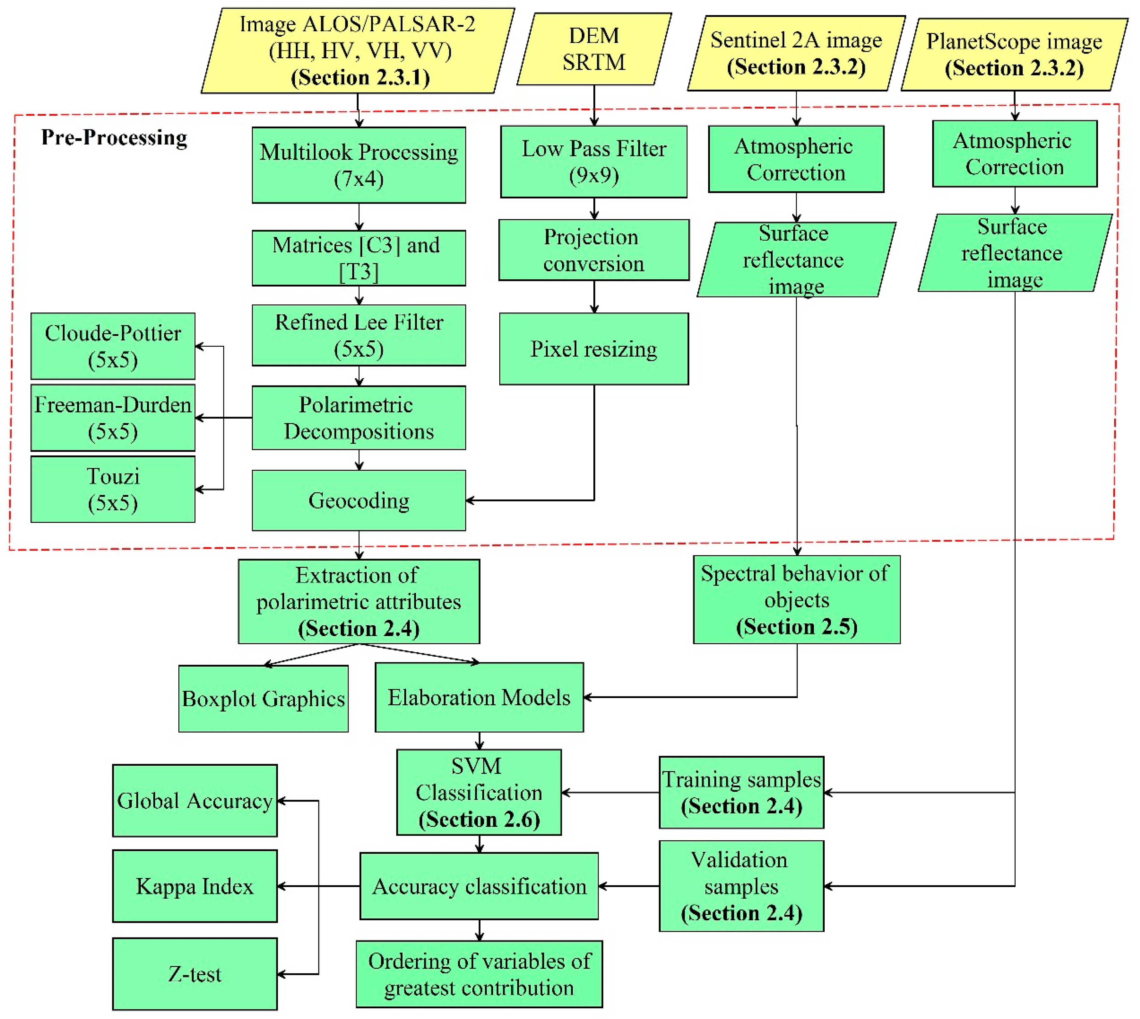
2.3. Image Processing
2.3.1. ALOS/PALSAR-2 Data Processing
2.3.2. SENTINEL-2A and PlanetScope Processing Steps
2.4. Selection of the Training and Validation Datasets and the Extraction of Polarimetric Attributes
2.5. Spectral Characterization of the Selected Land Use Classes Using SENTINEL-2A Image

| Extracted Attributes | Equation | Description | References |
|---|---|---|---|
| Backscatter coefficient , , 1 | , where | Indicates the orientation of the forest components. | [36,37] |
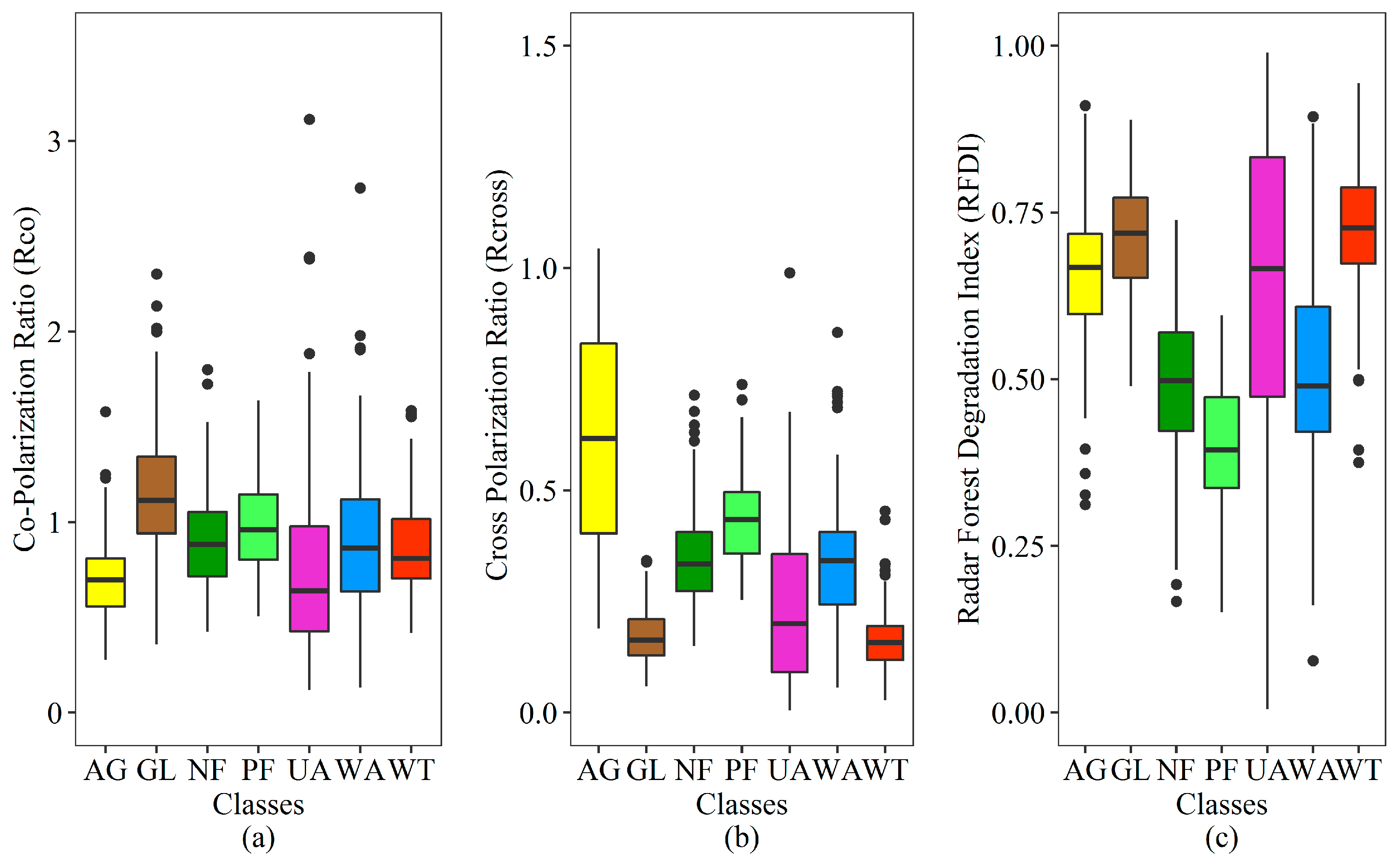
| Relation of Co-Polarization | Highlights different vertical and horizontal orientations derived from the structural aspects of vegetation. | [36] | |
| Cross Polarization Ratio | Sensitive to the volumetric dispersion of the forest to support classification and reduce topographic effects in backscattering. | [36] | |
| Radar Forest Degradation Index | Ratio designed to assess the strength of the double-bounce mechanism, which is useful for differentiating vegetation. | [38,39] | |
| Phase Difference 2 | Indication of the structure and quantity of biomass | [36] | |
| Entropy | ; | Related to the complexity of the forest structure. The most complex and diversified forest has high H, low A, and close to 45◦. | [40] |
| Anisotropy | |||
| Alpha Angle | |||
| Contribution of volume dispersion | Proportion of volumetric backscatter associated with the forest structure and biomass content. | [27] | |
| Double-bounce dispersion | Indication of canopy opening, density, and number of trees (trunks). | ||
| Surface dispersion | Related to the canopy opening. | ||
| Magnitude of type of Scattering ( | The magnitude is negatively correlated with biomass, with the tendency to single-bounce and various types of scattering. | [41] | |
| Phase of Scattering ( | Essential for an unambiguous description of the dispersion of the forest mechanism. | ||
| Orientation Angle (Ψ) | Compensate for the fluctuating influence of randomly oriented forest dispersal components and the slope of the land on scatters. | ||
| Helicity | Expresses the symmetry of forest dispersion, having an inverse correlation with biomass. |
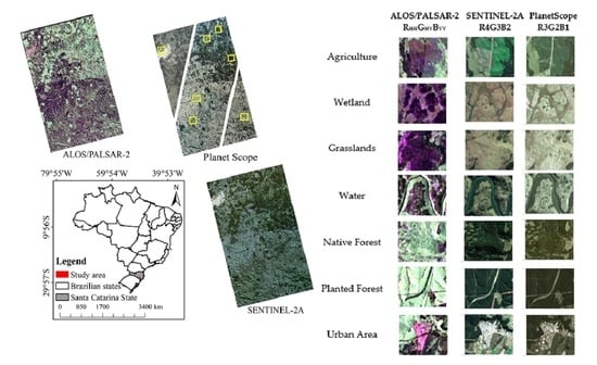
| Classes | Description | ALOS/PALSAR-2 | SENTINEL-2A | PlanetScope |
|---|---|---|---|---|
| RHHGHVBVV | R4G3B2 | R3G2B1 | ||
| Agriculture (AG) | Includes all cultivated land types (soybean, corn, beans, etc). |  |  |  |
| Wetland (WT) | Fragmented wet areas with floating or submerged vegetation. |  |  |  |
| Grasslands (GL) | Shrubby stratum, sparsely distributed on a grassy-woody carpet used for cattle ranching. |  |  |  |
| Water (WA) | It includes rivers, small streams, canals, natural lakes, artificial reservoirs, among others. |  |  |  |
| Native Forest (NF) | Vegetation areas covered by native forest and dominated with Araucaria trees. |  |  |  |
| Planted Forest (PF) | Vegetation areas covered by planted forest (Pinus sp. and Eucalyptus sp.). |  |  |  |
| Urban Area (UA) | Intensive use areas, structured by buildings and road system. |  |  |  |
2.6. Classification Evaluation based on Different Data Input Models
3. Results and Discussions
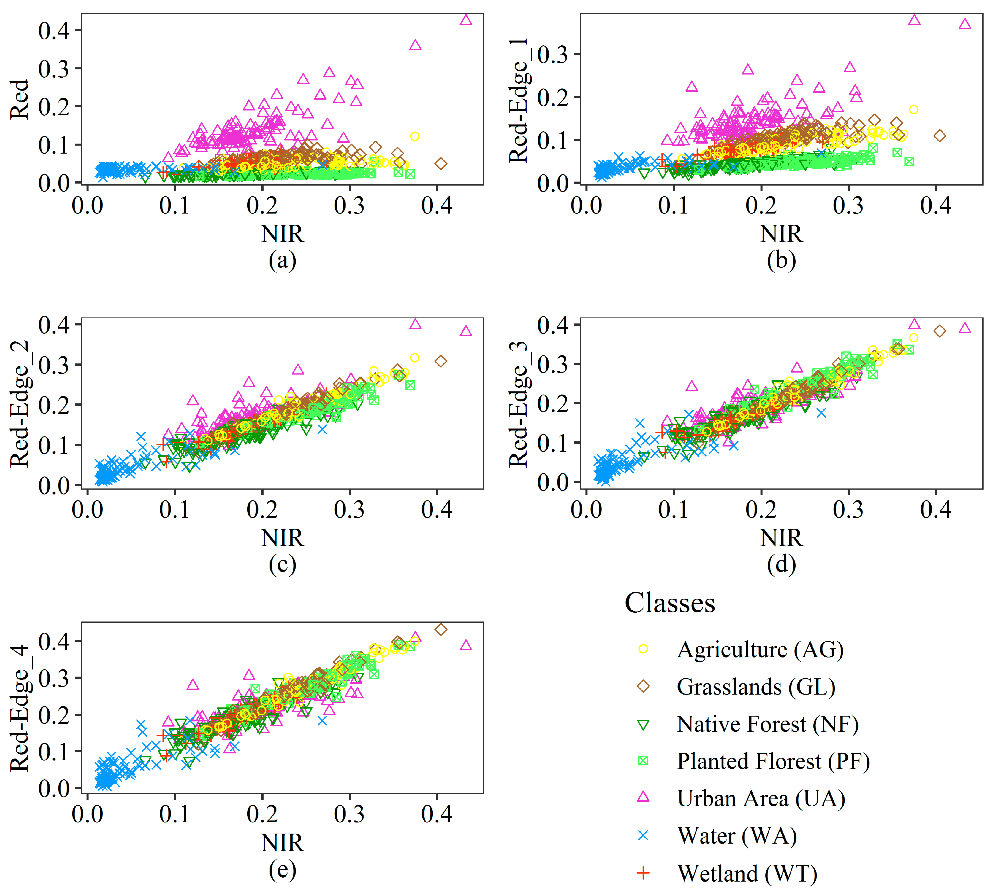
3.1. Spectral Behavior of Land Cover Classes of SENTINEL-2A Image
3.2. Discriminatory Analysis of Polarimetric Attributes from SAR Data
3.3. Classification of Land Cover Classes in Different Data Input Models
3.4. Importance of Features for Classification Accuracy
3.5. Further Research Perspectives
4. Conclusions
Author Contributions
Funding
Institutional Review Board Statement
Informed Consent Statement
Data Availability Statement
Acknowledgments
Conflicts of Interest
Appendix A. Methods and Results

| M1 | M2 | M3 | ||||
| Classes | UAc (%) | PAc (%) | UAc (%) | PAc (%) | UAc (%) | PAc (%) |
| AG | 37.50 | 6.49 | 46.55 | 38.67 | 70.45 | 50.03 |
| WT | 34.42 | 44.67 | 57.33 | 34.25 | 72.83 | 69.56 |
| GL | 30.80 | 86.69 | 55.32 | 84.74 | 67.72 | 82.73 |
| WA | 14.29 | 0.82 | 44.92 | 49.89 | 71.07 | 84.51 |
| NF | 32.14 | 23.35 | 48.31 | 55.78 | 55.88 | 69.40 |
| PF | 60.14 | 73.98 | 66.40 | 69.14 | 72.17 | 65.55 |
| UA | 60.00 | 27.95 | 90.16 | 26.68 | 90.00 | 31.26 |
| OA (%) | 37.48 | 53.93 | 68.43 | |||
| K (%) | 0.26 | 0.45 | 0.62 | |||
| M4 | M5 | M6 | ||||
| Classes | UAc (%) | PAc (%) | UAc (%) | PAc (%) | UAc (%) | PAc (%) |
| AG | 74.42 | 54.39 | 73.91 | 59.14 | 73.63 | 57.08 |
| WT | 73.00 | 74.68 | 75.26 | 76.05 | 74.23 | 74.64 |
| GL | 69.60 | 83.29 | 72.36 | 84.06 | 71.54 | 84.15 |
| WA | 71.30 | 78.65 | 73.87 | 79.96 | 72.17 | 80.43 |
| NF | 54.05 | 71.24 | 55.45 | 72.55 | 60.36 | 76.24 |
| PF | 75.47 | 61.92 | 72.90 | 60.57 | 77.14 | 64.67 |
| UA | 90.24 | 32.05 | 89.41 | 33.80 | 90.36 | 35.04 |
| OA (%) | 69.20 | 70.80 | 71.35 | |||
| K (%) | 0.63 | 0.65 | 0.66 | |||
| M7 | M8 | M9 | ||||
| Classes | UAc (%) | PAc (%) | UAc (%) | PAc (%) | UAc (%) | PAc (%) |
| AG | 86.41 | 83.09 | 89.00 | 77.93 | 91.00 | 87.53 |
| WT | 82.18 | 76.36 | 83.81 | 82.14 | 89.00 | 87.20 |
| GL | 80.37 | 89.47 | 83.33 | 90.92 | 88.68 | 92.89 |
| WA | 97.00 | 61.68 | 99.02 | 87.09 | 97.03 | 87.10 |
| NF | 88.07 | 97.43 | 88.18 | 97.84 | 88.99 | 97.63 |
| PF | 95.96 | 80.74 | 93.00 | 75.62 | 94.95 | 81.78 |
| UA | 95.28 | 73.16 | 100.00 | 86.97 | 92.73 | 87.44 |
| OA (%) | 85.56 | 87.44 | 90.29 | |||
| K (%) | 0.82 | 0.84 | 0.88 | |||
References
- Avtar, R.; Takeuchi, W.; Sawada, H. Full polarimetric PALSAR-based land cover monitoring in Cambodia for implementation of REDD policies. Int. J. Digit. Earth. 2013, 6, 255–275. [Google Scholar] [CrossRef]
- Furtado, L.F.A.; Silva, T.S.F.; Fernandes, P.J.F.; Novo, E.M.L.M. Land cover classification of Lago Grande de Curuai floodplain (Amazon, Brazil) using multi-sensor and image fusion techniques. Acta Amaz. 2015, 25, 195–202. [Google Scholar] [CrossRef] [Green Version]
- Pavanelli, J.A.P.; Santos, J.R.; Galvão, L.S.; Xaud, M.; Xaud, H.A.M. PALSAR-2/ALOS-2 and OLI/LANDSAT-8 data integration for land use and land cover mapping in northern Brazilian Amazon. Bol. Ciênc. Geod. 2018, 24, 250–269. [Google Scholar] [CrossRef]
- Souza Mendes, F.; Baron, D.; Gerold, G.; Liesenberg, V.; Erasmi, S. Optical and SAR Remote Sensing Synergism for Mapping Vegetation Types in the Endangered Cerrado/Amazon Ecotone of Nova Mutum—Mato Grosso. Remote Sens. 2019, 11, 1161. [Google Scholar] [CrossRef] [Green Version]
- Bamler, R. Principles of synthetic aperture radar. Surv. Geophys. 2000, 21, 147–157. [Google Scholar] [CrossRef]
- Chen, K.-S. Principles of Synthetic Aperture Radar Imaging: A System Simulation Approach; CRC Press: Boca Raton, FL, USA, 2016; p. 236. [Google Scholar]
- Bovenga, F. Special Issue Synthetic Aperture Radar (SAR) Techniques and Applications. Sensors 2020, 20, 1851. [Google Scholar] [CrossRef] [Green Version]
- Furtado, L.F.A.; Silva, T.S.F.; Novo, E.M.L.M. Dual-season and full-polarimetric C band SAR assessment for vegetation mapping in the Amazon várzea wetlands. Remote Sens. Environ. 2016, 174, 212–222. [Google Scholar] [CrossRef] [Green Version]
- Varghese, A.O.; Suryavanshi, A.; Joshi, A.K. Analysis of different polarimetric target decomposition methods in forest density classification using C band SAR data. Int. J. Remote Sens. 2016, 37, 694–709. [Google Scholar] [CrossRef]
- Camargo, F.F.; Sano, E.E.; Almeida, C.M.; Mura, J.C.; Almeida, T. A Comparative Assessment of Machine-Learning Techniques for Land Use and Land Cover Classification of the Brazilian Tropical Savanna Using ALOS-2/PALSAR-2 Polarimetric Images. Remote Sens. 2019, 11, 1600. [Google Scholar] [CrossRef] [Green Version]
- Wiederkehr, N.C.; Gama, F.F.; Mura, J.C.; Santos, J.R.; Bispo, P.C.; Sano, E.E. Analysis of the target decomposition technique attributes and polarimetric ratios to discriminate land use and land cover classes of the Tapajós region. Bol. Ciênc. Geod. 2019, 25, e2019002. [Google Scholar] [CrossRef]
- Parida, B.R.; Mandal, S.P. Polarimetric decomposition methods for LULC mapping using ALOS L-band PolSAR data in Western parts of Mizoram, Northeast India. SN Appl. Sci. 2020, 2, 1049. [Google Scholar] [CrossRef]
- Cassol, H.L.G.; Carreiras, J.M.B.; Moraes, E.C.; Aragão, L.E.O.C.; Silva, C.V.J.; Quegan, S.; Shimabukuro, Y.E. Retrieving Secondary Forest Aboveground Biomass from Polarimetric ALOS-2 PALSAR-2 Data in the Brazilian Amazon. Remote Sens. 2019, 11, 59. [Google Scholar] [CrossRef] [Green Version]
- De Freitas, D.M.; Sano, E.E.; DE Souza, R.A. Potential of multipolarized ALOS/PALSAR satellite images to discriminate vegetation coverage in the Pantanal biome: A case study in the region of Medio Taquari, MS. RBC 2014, 66, 209–221. [Google Scholar]
- Wiederkehr, N.C.; Gama, F.F.; Castro, P.B.N.; Bispo, P.C.; Balzter, H.; Sano, E.E.; Liesenberg, V.; Santos, J.R.; Mura, J.C. Discriminating Forest Successional Stages, Forest Degradation, and Land Use in Central Amazon Using ALOS/PALSAR-2 Full-Polarimetric Data. Remote Sens. 2020, 12, 3512. [Google Scholar] [CrossRef]
- Moran, M.S.; Hymer, D.C.; Qi, J.; Kerr, Y. Comparison of ERS-2 SAR and Landsat TM imagery for monitoring agricultural crop and soil conditions. Remote Sens. Environ. 2002, 79, 243–252. [Google Scholar] [CrossRef]
- Chaves, J.M.; Sano, E.E.; Guimarães, E.M.; Silva, A.S.; Meneses, P.R. Sinergismo entre dados ópticos e de radar para o estudo geológico na região de Bezerra-Cabeceiras, Goiás. RBG 2003, 33, 137–146. [Google Scholar] [CrossRef] [Green Version]
- Sano, E.; Santos, E.M.; Meneses, P.R. Análise de imagens do satélite ALOS PALSAR para o mapeamento de uso e cobertura da terra do Distrito Federal. Geociências 2009, 28, 441–451. [Google Scholar]
- Huang, S.; Potter, C.; Crabtree, R.L.; Hager, S.; Gross, P. Fusing optical and radar data to estimate sagebrush, herbaceous, and bare ground cover in Yellowstone. Remote Sens. Environ. 2010, 114, 251–264. [Google Scholar] [CrossRef]
- Pereira, L.D.O.; Freitas, C.C.; Sant’Anna, S.J.S.; Lu, D.; Moran, E.F. Optical and radar data integration for land use and land cover mapping in the Brazilian Amazon. GISci. Remote Sens. 2013, 50, 301–321. [Google Scholar] [CrossRef]
- Liesenberg, V.; de Filho, C.R.; Gloaguen, R. Evaluating moisture and geometry effects on L-Band SAR classification performance over a tropical rain forest environment. IEEE Trans. Geosci. Remote Sens. 2016, 9, 5357–5368. [Google Scholar] [CrossRef]
- De Magalhães, T.L.; Schimalski, M.B.; Mantovani, A.; Bortoluzzi, R.L.C. Image classification using Landsat TM images to mapping wetlands vegetation (banhados) of the Catarinense Plateau, Southern Brazil. In Proceedings of the 4th GEOBIA, Rio de Janeiro, Brazil, 7–9 May 2012. [Google Scholar]
- Polêse, C.; Oliveira, F.H.; Lima, C.L.; Alves, F.E. Análise da hidrografia da Coxilha Rica, Sul do município de Lages–SC Introdução. Geosul 2015, 30, 47–66. [Google Scholar] [CrossRef] [Green Version]
- Alvares, C.A.; Stape, J.L.; Sentelhas, P.C.; De Moraes Gonçalves, J.L.; Sparovek, G. Köppen’s climate classification map for Brazil. Meteorol. Z. 2013, 22, 711–728. [Google Scholar] [CrossRef]
- IBGE. Mapa de Vegetação do Brasil, 3rd ed.; Instituto Brasileiro de Geografia e Estatística: Rio de Janeiro, Brazil, 1993. Available online: Ftp://ftp.ibge.gov.br/Cartas_e_Mapas/Mapas_Murais/ (accessed on 3 March 2020).
- ANA-Agência Nacional De Águas. HidroWeb: Sistema de Informações Hidrológicas. Available online: http://hidroweb.ana.gov.br (accessed on 5 March 2020).
- Freeman, A.; Durden, S.L. A Three-component scattering model for polarimetric SAR data. IEEE Trans. Geosci. Remote Sens. 1998, 36, 963–973. [Google Scholar] [CrossRef] [Green Version]
- Cloude, S.R. Group theory and polarisation algebra. Optik 1986, 75, 26–36. [Google Scholar]
- Lee, J.-S.; Pottier, E. Polarimetric Radar Imaging from Basics to Applications; CRC Press: Boca Raton, FL, USA, 2009; p. 438. [Google Scholar]
- Qiu, F.; Berglund, J.; Jensen, J.R.; Thakkar, P.; Ren, D. Speckle Noise Reduction in SAR Imagery Using a Local Adaptive Median Filter. GISci. Remote Sens. 2004, 41, 244–266. [Google Scholar] [CrossRef] [Green Version]
- Mishra, V.N.; Prasad, R.; Kumar, P.; Gupta, D.K.; Srivastava, P.K. Dual-polarimetric C-band SAR data for land use/land cover classification by incorporating textural information. Environ. Earth Sci. 2017, 76, 26. [Google Scholar] [CrossRef]
- ESA. PolSARpro v6.0 (Biomass Edition) Toolbox. Available online: https://step.esa.int/main/toolboxes/polsarpro-v6-0-biomass-edition-toolbox/ (accessed on 26 July 2020).
- Meneses, P.R.; Almeida, T.D. Introdução ao Processamento de Imagens de Sensoriamento Remoto; UNB: Brasília, Brasil, 2012; p. 266. [Google Scholar]
- Müller-Wilm, U.; Devignot, O.; Pessiot, L. Sen2Cor Configuration and User Manual-S2-PDGS-MPC-L2A-SUM-V2.4. Available online: https://step.esa.int/thirdparties/sen2cor/2.4.0/Sen2Cor_240_Documenation_PDF/S2-PDGS-MPC-L2A-SUM-V2.4.0.pdf (accessed on 11 April 2020).
- Rstudio Team. RStudio: Integrated Development for R. RStudio. Available online: http://www.rstudio.com/ (accessed on 7 April 2020).
- Henderson, F.M.; Lewis, A.J. Principles and Applications of Imaging Radar, 3rd ed.; Wiley: Hoboken, NJ, USA, 1998; p. 896. [Google Scholar]
- Shimada, M.; Isoguchi, O.; Tadono, T.; Isono, K. Palsar radiometric and geometric calibration. IEEE Trans. Geosci. Remote Sens. 2009, 47, 3915–3932. [Google Scholar] [CrossRef]
- Saatchi, S.S.; Dubayah, R.; Clark, D.; Chazdon, R.; Hollinger, D. Estimation of forest biomass change from fusion of radar and lidar measurements. Available online: http://www.slideshare.net/grssieee/estimation-offorest-biomass (accessed on 7 April 2020).
- Mitchard, E.T.A.; Saatchi, S.S.; White, L.J.T.; Abernethy, K.A.; Jeffery, K.J.; Lewis, S.L.; Collins, M.; Lefsky, M.A.; Leal, M.E.; Woodhouse, I.H. Mapping tropical forest biomass with radar and spaceborne LiDAR in Lopé National Park, Gabon: Overcoming problems of high biomass and persistent cloud. Biogeosciences 2012, 9, 179–191. [Google Scholar] [CrossRef] [Green Version]
- Cloude, S.R.; Pottier, E. An entropy based classification scheme for land applications of polarimetric SAR. IEEE Trans. Geosci. Remote Sens. 1997, 35, 68–78. [Google Scholar] [CrossRef]
- Touzi, R. Target scattering decomposition in terms of roll-invariant target parameters. IEEE Trans. Geosci. Remote Sens. 2007, 45, 73–84. [Google Scholar] [CrossRef]
- Attarchi, S.; Gloaguen, R. Classifying Complex Mountainous Forests with L-Band SAR and Landsat Data Integration: A Comparison among Different Machine Learning Methods in the Hyrcanian Forest. Remote Sens. 2014, 6, 3624–3647. [Google Scholar] [CrossRef] [Green Version]
- Üstüner, M.; Gökdağ, Ü.; Bilgin, G.; Şanlı, F.B. Comparing the classification performances of supervised classifiers with balanced and imbalanced SAR data sets. In Proceedings of the Signal Processing and Communications Applications Conference (SIU), Izmir, Turkey, 2–5 May 2018; IEEE: Piscataway, NJ, USA, 2018. [Google Scholar]
- Vapnik, V.N. Statistical Learning Theory; Wiley: Hoboken, NJ, USA, 1998; p. 768. [Google Scholar]
- Li, W.; Du, Q. Support vector machine with adaptive composite kernel for hyperspectral image classification. In Satellite Data Compression, Communications, and Processing XI; International Society for Optics and Photonics: Baltimore, MD, USA, 2015. [Google Scholar]
- Van der Linden, S.; Rabe, A.; Held, M.; Jakimow, B.; Leitão, P.J.; Okujeni, A.; Schwieder, M.; Suess, S.; Hostert, P. The EnMAP-Box—A Toolbox and Application Programming Interface for EnMAP Data Processing. Remote Sens. 2015, 7, 11249–11266. [Google Scholar] [CrossRef] [Green Version]
- Olofsson, P.; Foody, G.M.; Stehman, S.V.; Woodcock, C.E. Making better use of accuracy data in land change studies: Estimating accuracy and area and quantifying uncertainty using stratified estimation. Remote Sens. Environ. 2014, 129, 122–131. [Google Scholar] [CrossRef]
- Olofsson, P.; Foody, G.M.; Herold, M.; Stehman, S.V.; Woodcock, C.E.; Wulder, M.A. Good practices for estimating area and assessing accuracy of land change. Remote Sens. Environ. 2014, 148, 42–57. [Google Scholar] [CrossRef]
- Herold, M.; Gardner, M.E.; Roberts, D.A. Spectral resolution requirements for mapping urban areas. IEEE Trans. Geosci. Remote Sens. 2003, 41, 1907–1919. [Google Scholar] [CrossRef] [Green Version]
- Radoux, J.; Chomé, G.; Jacques, D.C.; Waldner, F.; Bellemans, N.; Matton, N.; Lamarche, C.; D’Andrimont, R.; Defourny, P. Sentinel-2′s Potential for Sub-Pixel Landscape Feature Detection. Remote Sens. 2016, 8, 488. [Google Scholar] [CrossRef] [Green Version]
- Sothe, C.; Almeida, C.M.; Liesenberg, V.; Schimalski, M.B. Evaluating Sentinel-2 and Landsat-8 Data to Map Sucessional Forest Stages in a Subtropical Forest in Southern Brazil. Remote Sens. 2017, 9, 838. [Google Scholar] [CrossRef] [Green Version]
- Prieto-Amparan, J.A.; Villarreal-Guerrero, F.; Martinez-Salvador, M.; Manjarrez-Domínguez, C.; Santellano-Estrada, E.; Pinedo-Alvarez, A. Atmospheric and Radiometric Correction Algorithms for the Multitemporal Assessment of Grasslands Productivity. Remote Sens. 2018, 10, 219. [Google Scholar] [CrossRef] [Green Version]
- Ettehadi Osgouei, P.; Kaya, S.; Sertel, E.; Alganci, U. Separating Built-Up Areas from Bare Land in Mediterranean Cities Using Sentinel-2A Imagery. Remote Sens. 2019, 11, 345. [Google Scholar] [CrossRef] [Green Version]
- Kuplich, T.M. Estudos florestais com imagens de radar. Espaç. Geogr. 2003, 6, 65–90. [Google Scholar]
- Kasischke, E.S.; Bourgeau-Chavez, L.L. Monitoring South Florida wetlands using ERS-1 SAR imagery. Photogramm Eng. Remote Sens. 1997, 63, 281–291. [Google Scholar]
- Leckie, D.G.; Ranson, K.J. Forest applications using imaging radar. In Principles and Applications of Imaging Radar, 3rd ed.; Henderson, F.M., Lewis, A.J., Eds.; Wiley: Hoboken, NJ, USA, 1998; Volume 2, pp. 435–509. [Google Scholar]
- Formaggio, A.R.; Epiphanio, J.C.N.; Simões, M.D.S. Radarsat backscattering from an agricultural scene. Pesq. Agropec. Bras. 2001, 36, 823–830. [Google Scholar] [CrossRef] [Green Version]
- Oliver, C.J.; Quegan, S. Understanding Synthetic Aperture Radar Images; Scitech Publishing: Raleigh, NC, USA, 2004; p. 512. [Google Scholar]
- Martins, F.D.; Santos, J.R.; Galvão, L.S.; Xaud, H.A. Sensitivity of ALOS/PALSAR imagery to forest degradation by fire in northern Amazon. Int. J. Appl. Earth Obs. Geoinf. 2016, 49, 49–163. [Google Scholar] [CrossRef]
- Cloude, S.R.; Pottier, E. A review of target decomposition theorems in Radar Polarimetry. IEEE Trans. Geosci. Remote Sens. 1996, 34, 498–518. [Google Scholar] [CrossRef]
- Zou, T.; Yang, W.; Dai, D.; Sun, H. Polarimetric SAR image classification using multifeatures combination and combination and extremely randomized clustering forests. EURASIP J. Adv. Signal Process. 2009, 2010, 465612. [Google Scholar] [CrossRef] [Green Version]
- Longepe, N.; Rakwatin, P.; Isoguchi, M.; Shimada, M.; Uryu, Y.; Yulianto, K. Assessment of ALOS PALSAR 50 m orthorectified FBD data for regional land cover classification by support vector machines. IEEE Trans. Geosci. Remote Sens. 2011, 262, 1786–1798. [Google Scholar] [CrossRef]
- Attarchi, S. Extracting impervious surfaces from full polarimetric SAR images in different urban areas. Int. J. Remote Sens. 2020, 41, 4644–4663. [Google Scholar] [CrossRef]
- Guimarães, U.S.; Galo, M.L.B.T.; Narvaes, I.S.; Silva, A.Q. Cosmo-SkyMed and TerraSAR-X datasets for geomorphological mapping in the eastern of Marajó Island, Amazon coast. Geomorphology 2020, 350, 106934. [Google Scholar] [CrossRef]
- Pulella, A.; Aragão Santos, R.; Sica, F.; Posovszky, P.; Rizzoli, P. Multi-Temporal Sentinel-1 Backscatter and Coherence for Rainforest Mapping. Remote Sens. 2020, 12, 847. [Google Scholar] [CrossRef] [Green Version]
- Voormansik, K.; Zalite, K.; Sünter, I.; Tamm, T.; Koppel, K.; Verro, T.; Brauns, A.; Jakovels, D.; Praks, J. Separability of Mowing and Ploughing Events on Short Temporal Baseline Sentinel-1 Coherence Time Series. Remote Sens. 2020, 12, 3784. [Google Scholar] [CrossRef]
- Almeida, J.A.; Albuquerque, J.A.; Bortoluzzi, R.L.C.; Mantovani, A. Caracterização dos solos e da vegetação de áreas palustres (brejos e banhados) do Planalto Catarinense. Available online: http://solos-sc.com.br/index.php/conteudo/file/174-relatorio%20final_caracterizacao%20dos%20solos%20e%20da%20vegetacao%20de%20areas%20palustres-brejos%20e%20banhados-%20do%20planalto%20catarinense (accessed on 7 April 2020). (In Portuguese).
- Pal, M.; Foody, G.M. Feature selection for classification of hyperspectral data by SVM. IEEE Trans. Geosci. Remote Sens. 2010, 48, 2297–2307. [Google Scholar] [CrossRef] [Green Version]
- Rabe, A.; Van Der Linden, S.; Hostert, P. Simplifying support vector machines for classification of hyperspectral imagery and selection of relevant features. In Proceedings of the 2nd Workshop on Hyperspectral Image and Signal Processing: Evolution in Remote Sensing, Reykjavik, Iceland, 14–16 June 2010; IEEE: Piscataway, NJ, USA, 2010. [Google Scholar]
- Waske, B.; Van Der Linden, S.; Benediktsson, J.A.; Rabe, A.; Hostert, P. Sensitivity of support vector machines to random feature selection in classification of hyperspectral data. IEEE Trans. Geosci. Remote Sens. 2010, 48, 2880–2889. [Google Scholar] [CrossRef] [Green Version]
- van Beijma, S.; Chatterton, J.; Page, S.; Rawlings, C.; Tiffin, R.; King, H. The challenges of using satellite data sets to assess historical land use change and associated greenhouse gas emissions: A case study of three Indonesian provinces. Carbon Manag. 2018, 9, 399–413. [Google Scholar] [CrossRef] [Green Version]


| (a) ALOS/PALSAR-2 | |
| Acquisition Date | 02/23/2018 (experimental mode) |
| Wavelength | (approx. 23 cm) L band |
| Operating mode | Full Polarimetric (PLR) |
| Polarizations | Quad-pol (HH, VV, HV, VH) |
| Orbit | Ascending |
| Pixel spacing | 2.79m (range) × 2.86m (azimuth) |
| Angle of incidence | 33.2° |
| Final spatial resolution | 20 m in range × 20 m in azimuth |
| Number of rows and columns | 25,960 × 8816 |
| (b) PlanetScope | |
| Acquisition Date | 02/23/2018 |
| Central wavelength (nm) | VIS: 485, 545, 630 nm.Near-infrared(NIR): 820 nm |
| Spatial resolution (m) | ~3.0 |
| Radiometric resolution (bits) | 12 |
| Temporal resolution | Daily |
| (c) SENTINEL-2A | |
| Acquisition Date | 06/09/2018 |
| Central Wavelength (nm)/Spatial Resolution | 10 m: VIS (B2: 492.4, B3: 559.8, B4: 664.6), NIR (B8: 832.8) 20 m: red-edge (B5: 704.1, B6: 740.5, B7: 782.8), NIR (B8A: 864.7), shortwave-infrared (SWIR) (B11: 1613.7, B12: 2202.4) |
| Radiometric resolution (bits) | 12 |
| Temporal resolution | 10 days |
| Model | Data Input | Feature 1 | Number of features |
|---|---|---|---|
| M1 | SAR | 4 | |
| M2 | SAR | M1 + (H, A, α) | 7 |
| M3 | SAR | M2 + (Pv, Pd, Ps) | 10 |
| M4 | SAR | M3 + (, , Ψ,) | 14 |
| M5 | SAR | M4 + (Rco, Rcroos, RFDI) | 17 |
| M6 | SAR | M5 + ( | 20 |
| M7 | Optical | B02, B03, B04, B05, B06, B07, B08, B11, B12, B8A | 10 |
| M8 | Optical/SAR | M7 + M1 | 14 |
| M9 | Optical/SAR | M7 + M6 | 30 |
| (a) Weighted Overall Accuracy | |||||||||
| M1 | M2 | M3 | M4 | M5 | M6 | M7 | M8 | M9 | |
| OA | 0.3748 | 0.5393 | 0.6843 | 0.6920 | 0.7080 | 0.7135 | 0.8556 | 0.8744 | 0.9029 |
| Var(OA) | 0.0003 | 0.0004 | 0.0003 | 0.0003 | 0.0003 | 0.0003 | 0.0003 | 0.0002 | 0.0002 |
| Lower limit | 0.3396 | 0.5004 | 0.6480 | 0.6561 | 0.6727 | 0.6782 | 0.8233 | 0.8448 | 0.8770 |
| Upper limit | 0.4100 | 0.5781 | 0.7206 | 0.7279 | 0.7433 | 0.7489 | 0.8879 | 0.9040 | 0.9288 |
| (b) Weighted Kappa Index | |||||||||
| M1 | M2 | M3 | M4 | M5 | M6 | M7 | M8 | M9 | |
| Kappa | 0.2638 | 0.4520 | 0.6242 | 0.6333 | 0.6522 | 0.6587 | 0.8177 | 0.8439 | 0.8804 |
| Var(K) | 0.0002 | 0.0002 | 0.0003 | 0.0003 | 0.0003 | 0.0003 | 0.0003 | 0.0003 | 0.0003 |
| Lower limit | 0.2363 | 0.4214 | 0.5930 | 0.6020 | 0.6209 | 0.6273 | 0.7817 | 0.8095 | 0.8464 |
| Upper limit | 0.2912 | 0.4826 | 0.6555 | 0.6646 | 0.6836 | 0.6900 | 0.8537 | 0.8784 | 0.9144 |
| M1 | M2 | M3 | M4 | M5 | M6 | M7 | M8 | M9 | |
|---|---|---|---|---|---|---|---|---|---|
| M1 | - | 8.97 | 16.99 | 17.40 | 18.27 | 18.57 | 23.99 | 25.80 | 27.66 |
| M2 | - | - | 7.72 | 8.12 | 8.96 | 9.24 | 15.17 | 16.66 | 18.35 |
| M3 | - | - | - | 0.40 1 | 1.24 1 | 1.52 1 | 7.96 | 9.26 | 10.88 |
| M4 | - | - | - | - | 1.92 | 1.12 1 | 7.58 | 8.87 | 10.48 |
| M5 | - | - | - | - | - | 0.28 1 | 6.80 | 8.06 | 9.67 |
| M6 | - | - | - | - | - | - | 6.53 | 7.79 | 9.40 |
| M7 | - | - | - | - | - | - | - | 1.03 1 | 2.48 |
| M8 | - | - | - | - | - | - | - | - | 1.48 1 |
| M1 | M2 | M3 | ||||
| Classes | Area (km2) | % land cover | Area (km2) | % land cover | Area (km2) | % land cover |
| AG | 77.47 | 2.64 | 347.13 | 11.81 | 301.00 | 10.24 |
| WT | 569.43 | 19.38 | 268.92 | 9.15 | 528.30 | 17.98 |
| GL | 1397.71 | 47.57 | 922.78 | 31.40 | 674.80 | 22.96 |
| WA | 26.91 | 0.92 | 471.54 | 16.05 | 569.22 | 19.37 |
| NF | 282.41 | 9.61 | 493.20 | 16.78 | 523.24 | 17.81 |
| PF | 416.28 | 14.17 | 352.81 | 12.01 | 267.30 | 9.10 |
| UA | 168.25 | 5.73 | 82.09 | 2.79 | 74.60 | 2.54 |
| Total | 2938.47 | 100.00 | 2938.47 | 100.00 | 2938.47 | 100.00 |
| M4 | M5 | M6 | ||||
| Classes | Area (km2) | % land cover | Area (km2) | % land cover | Area (km2) | % land cover |
| AG | 315.04 | 10.72 | 342.79 | 11.67 | 329.39 | 11.21 |
| WT | 575.82 | 19.60 | 580.98 | 19.77 | 574.44 | 19.55 |
| GL | 640.47 | 21.80 | 621.06 | 21.14 | 640.20 | 21.79 |
| WA | 536.39 | 18.25 | 533.16 | 18.14 | 531.91 | 18.10 |
| NF | 547.41 | 18.63 | 532.38 | 18.12 | 534.82 | 18.20 |
| PF | 252.24 | 8.58 | 254.45 | 8.66 | 250.90 | 8.54 |
| UA | 71.11 | 2.42 | 73.65 | 2.51 | 76.82 | 2.61 |
| Total | 2938.47 | 100.00 | 2938.47 | 100.00 | 2938.47 | 100.00 |
| M7 | M8 | M9 | ||||
| Classes | Area (km2) | % land cover | Area (km2) | % land cover | Area (km2) | % land cover |
| AG | 312.06 | 10.62 | 290.25 | 9.88 | 340.20 | 11.58 |
| WT | 591.14 | 20.12 | 569.74 | 19.39 | 644.20 | 21.92 |
| GL | 847.41 | 28.84 | 791.72 | 26.94 | 729.80 | 24.84 |
| WA | 65.54 | 2.23 | 148.45 | 5.05 | 189.27 | 6.44 |
| NF | 794.10 | 27.02 | 795.35 | 27.07 | 699.20 | 23.79 |
| PF | 280.16 | 9.53 | 251.22 | 8.55 | 261.90 | 8.91 |
| UA | 48.07 | 1.64 | 91.75 | 3.12 | 73.90 | 2.51 |
| Total | 2938.47 | 100.00 | 2938.47 | 100.00 | 2938.47 | 100.00 |
| M6 | M9 | |||
|---|---|---|---|---|
| Classification | Feature | Overall Acc. | Feature | Overall Acc. |
| 1 | Pv | 40.88 | B12 | 47.5 |
| 2 | Pd | 55.77 | Pv | 69.01 |
| 3 | A | 65.83 | B8A | 79.17 |
| 4 | α_s | 69.22 | Ps | 83.47 |
| 5 | ϕ_αs | 70.85 | B05 | 85.92 |
| 6 | HH | 72.3 | B11 | 87.74 |
| 7 | Rcroos | 72.59 | RFDI | 88.73 |
| 8 | VV | 73.68 | α_s | 89.14 |
| 9 | H | 73.75 | B07 | 89.46 |
| 10 | ∆(HH-HV) | 74.02 | H | 89.71 |
| 11 | HV | 74.19 | B4 | 90.06 |
| 12 | Pd | 74.21 | B2 | 90.13 |
| 13 | α | 74.69 | VV | 90.24 |
| 14 | VH | 74.9 | α | 90.48 |
| 15 | τ_m | 75.24 | VH | 90.65 |
| 16 | ∆(HV-VV) | 75.09 | ∆(HH-VV) | 90.6 |
| 17 | RFDI | 74.82 | Pd | 90.42 |
| 18 | Ψ | 74.22 | Rcroos | 90.5 |
| 19 | ∆(HH-VV) | 74.38 | ∆(HH-HV) | 90.38 |
| 20 | Rco | 73.7 | B06 | 90.34 |
| 21 | - | - | τ_m | 90.57 |
| 22 | - | - | ϕ_αs | 90.51 |
| 23 | - | - | A | 90.54 |
| 24 | - | - | Ψ | 90.26 |
| 25 | - | - | ∆(HV-VV) | 89.89 |
| 26 | - | - | Rco | 89.65 |
| 27 | - | - | HV | 89.78 |
| 28 | - | - | B03 | 89.68 |
| 29 | - | - | B08 | 89.49 |
| 30 | - | - | HH | 89.75 |
Publisher’s Note: MDPI stays neutral with regard to jurisdictional claims in published maps and institutional affiliations. |
© 2021 by the authors. Licensee MDPI, Basel, Switzerland. This article is an open access article distributed under the terms and conditions of the Creative Commons Attribution (CC BY) license (http://creativecommons.org/licenses/by/4.0/).
Share and Cite
Costa, J.d.S.; Liesenberg, V.; Schimalski, M.B.; Sousa, R.V.d.; Biffi, L.J.; Gomes, A.R.; Neto, S.L.R.; Mitishita, E.; Bispo, P.d.C. Benefits of Combining ALOS/PALSAR-2 and Sentinel-2A Data in the Classification of Land Cover Classes in the Santa Catarina Southern Plateau. Remote Sens. 2021, 13, 229. https://doi.org/10.3390/rs13020229
Costa JdS, Liesenberg V, Schimalski MB, Sousa RVd, Biffi LJ, Gomes AR, Neto SLR, Mitishita E, Bispo PdC. Benefits of Combining ALOS/PALSAR-2 and Sentinel-2A Data in the Classification of Land Cover Classes in the Santa Catarina Southern Plateau. Remote Sensing. 2021; 13(2):229. https://doi.org/10.3390/rs13020229
Chicago/Turabian StyleCosta, Jessica da Silva, Veraldo Liesenberg, Marcos Benedito Schimalski, Raquel Valério de Sousa, Leonardo Josoé Biffi, Alessandra Rodrigues Gomes, Sílvio Luís Rafaeli Neto, Edson Mitishita, and Polyanna da Conceição Bispo. 2021. "Benefits of Combining ALOS/PALSAR-2 and Sentinel-2A Data in the Classification of Land Cover Classes in the Santa Catarina Southern Plateau" Remote Sensing 13, no. 2: 229. https://doi.org/10.3390/rs13020229