sUAS Remote Sensing to Evaluate Geothermal Seep Interactions with the Yellowstone River, Montana, USA

Abstract
:
1. Introduction
2. Methods
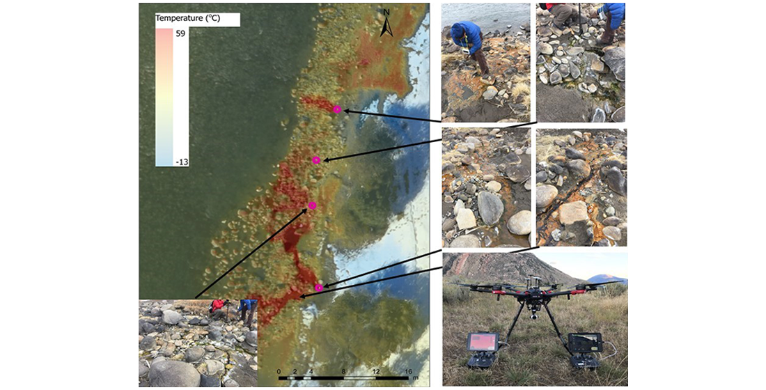
2.1. Study Site
2.2. Field Methods and Data Acquisition
2.2.1. RGB and TIR Image Acquisition
2.2.2. Ground Truth and Water Elevation Data
2.2.3. Stream Bed Vertical Temperature Profiles
2.3. Data Analysis
2.3.1. SfM Photogrammetry
2.3.2. TIR Image Temperature Data Transformation, Accuracy, and Feature Identification
2.3.3. DSM Water Surface Elevation Accuracy and Water Depth Rating Curve
2.3.4. Seepage Flux
3. Results
3.1. SfM Photogrammetry
3.1.1. RGB Orthomosaic and DSM Accuracy
3.1.2. Thermal Orthomosaic Accuracy and Feature Identification
Evaluation of Collocated Temperature Variation
3.2. DSM Water Surface Elevation Accuracy
3.3. Seepage Flux
4. Discussion
4.1. RGB and TIR SfM Photogrammetry Utility and Limitations for Fluvial Environments
4.2. Hydrothermal Seep Dynamics
4.3. Limitations
5. Conclusions
Author Contributions
Funding
Data Availability Statement
Acknowledgments
Conflicts of Interest
Appendix A


References
- Niedzielski, T.; Witek, M.; Spallek, W. Observing river stages using unmanned aerial vehicles. Hydrol. Earth Syst. Sci. 2016, 20, 3193–3205. [Google Scholar] [CrossRef] [Green Version]
- Ridolfi, E.; Manciola, P. Water Level Measurements from Drones: A Pilot Case Study at a Dam Site. Water 2018, 10, 297. [Google Scholar] [CrossRef] [Green Version]
- Rivas Casado, M.; Ballesteros Gonzalez, R.; Wright, R.; Bellamy, P. Quantifying the effect of aerial imagery resolution in automated hydromorphological river characterization. Remote Sens. 2016, 8, 650. [Google Scholar] [CrossRef] [Green Version]
- Woodget, A.S.; Visser, F.; Maddock, I.P.; Carbonneau, P.E. The Accuracy and Reliability of Traditional Surface Flow Type Mapping: Is it Time for a New Method of Characterizing Physical River Habitat? River Res. Appl. 2016, 32, 1902–1914. [Google Scholar] [CrossRef] [Green Version]
- Woodget, A.S.; Austrums, R.; Maddock, I.P.; Habit, E. Drones and digital photogrammetry: From classifications to continuums for monitoring river habitat and hydromorphology. Wiley Interdiscip. Rev. Water 2017, 4, e1222. [Google Scholar] [CrossRef] [Green Version]
- Bagheri, O.; Ghodsian, M.; Saadatseresht, M. Reach scale application of UAV+ SfM method in shallow rivers hy-perspatial bathymetry. The International Archives of Photogrammetry. Remote Sens. Spatial Inform. Sci. 2015, 40, 77. [Google Scholar]
- Woodget, A.S.; Carbonneau, P.E.; Visser, F.; Maddock, I.P. Quantifying submerged fluvial topography using hy-perspatial resolution UAS imagery and structure from motion photogrammetry. Earth Surf. Process. Landf. 2015, 40, 47–64. [Google Scholar] [CrossRef] [Green Version]
- Aicardi, I.; Chiabrando, F.; Lingua, A.M.; Noardo, F.; Piras, M.; Vigna, B. A methodology for acquisition and pro-cessing of thermal data acquired by UAVs: A test about subfluvial springs’ investigations. Geomatics. Nat. Hazards Risk 2017, 8, 5–17. [Google Scholar] [CrossRef] [Green Version]
- Abolt, C.; Caldwell, T.; Wolaver, B.; Pai, H. Unmanned aerial vehicle-based monitoring of groundwater inputs to surface waters using an economical thermal infrared camera. Opt. Eng. 2018, 57, 053113. [Google Scholar] [CrossRef]
- Briggs, M.A.; Dawson, C.B.; Holmquist-Johnson, C.; Williams, K.H.; Lane, J.W., Jr. Efficient hydrogeological char-acterization of remote stream corridors using drones. Hydrol. Process. 2019, 33, 316–319. [Google Scholar] [CrossRef] [Green Version]
- Chacon, D.C. Thermal Infrared Remote Sensing for Water Temperature Assessment along the Santa Ana River Using an Unmanned Aerial Vehicle (UAV) System. Ph.D. Thesis, California State University, Fullerton, CA, USA, 2019. [Google Scholar]
- Ullman, S. The interpretation of structure from motion. Proceedings of the Royal Society of London. Ser. B Biol. Sci. 1979, 203, 405–426. [Google Scholar]
- Kalacska, M.; Chmura, G.; Lucanus, O.; Bérubé, D.; Arroyo-Mora, J. Structure from motion will revolutionize analyses of tidal wetland landscapes. Remote. Sens. Environ. 2017, 199, 14–24. [Google Scholar] [CrossRef]
- Döpper, V.; Gränzig, T.; Kleinschmit, B.; Förster, M. Challenges in UAS-Based TIR Imagery Processing: Image Alignment and Uncertainty Quantification. Remote. Sens. 2020, 12, 1552. [Google Scholar] [CrossRef]
- Dugdale, S.J.; Malcolm, I.A.; Hannah, D.M. Drone-based Structure-from-Motion provides accurate forest canopy data to assess shading effects in river temperature models. Sci. Total Environ. 2019, 678, 326–340. [Google Scholar] [CrossRef] [PubMed]
- Jaworowski, C.; Heasler, H.; Neale, C.M.U.; Saravanan, S.; Masih, A. Temporal and Seasonal Variations of the Hot Spring Basin Hydrothermal System, Yellowstone National Park, USA. Remote Sens. 2013, 5, 6587–6610. [Google Scholar] [CrossRef] [Green Version]
- Neale, C.M.U.; Jaworowski, C.; Heasler, H.; Sivarajan, S.; Masih, A. Hydrothermal monitoring in Yellowstone National Park using airborne thermal infrared remote sensing. Remote Sens. Environ. 2016, 184, 628–644. [Google Scholar] [CrossRef] [Green Version]
- Ingebritsen, S.; Galloway, D.L.; Colvard, E.; Sorey, M.; Mariner, R. Time-variation of hydrothermal discharge at selected sites in the western United States: Implications for monitoring. J. Volcanol. Geotherm. Res. 2001, 111, 1–23. [Google Scholar] [CrossRef]
- Boylen, C.W.; Brock, T.D. Effects of Thermal Additions from the Yellowstone Geyser Basins on the Benthic Algae of the Firehole River. Ecology 1973, 54, 1282–1291. [Google Scholar] [CrossRef]
- Garrott, R.A.; Eberhardt, L.L.; Otton, J.K.; White, P.J.; Chaffee, M.A. A geochemical trophic cascade in Yellow-stone’s geothermal environments. Ecosystems 2002, 5, 0659–0666. [Google Scholar] [CrossRef]
- Jensen, A.M.; Neilson, B.T.; McKee, M.; Chen, Y. Thermal remote sensing with an autonomous unmanned aerial remote sensing platform for surface stream temperatures. In Proceedings of the 2012 IEEE International Geoscience and Remote Sensing Symposium, Munich, Germany, 22–27 July 2012; pp. 5049–5052. [Google Scholar]
- Wawrzyniak, V.; Piégay, H.; Allemand, P.; Vaudor, L.; Grandjean, P. Prediction of water temperature heterogeneity of braided rivers using very high resolution thermal infrared (TIR) images. Int. J. Remote. Sens. 2013, 34, 4812–4831. [Google Scholar] [CrossRef]
- Dugdale, S.J.; Kelleher, C.; Malcolm, I.A.; Caldwell, S.; Hannah, D.M. Assessing the potential of drone-based thermal infrared imagery for quantifying river temperature heterogeneity. Hydrol. Process. 2019, 33, 1152–1163. [Google Scholar] [CrossRef]
- Loheide, S.P.; Gorelick, S.M. Quantifying Stream—Aquifer Interactions through the Analysis of Remotely Sensed Thermographic Profiles and In Situ Temperature Histories. Environ. Sci. Technol. 2006, 40, 3336–3341. [Google Scholar] [CrossRef]
- Schuetz, T.; Weiler, M. Quantification of localized groundwater inflow into streams using ground-based infrared thermography. Geophys. Res. Lett. 2011, 38. [Google Scholar] [CrossRef]
- Hare, D.K.; Briggs, M.A.; Rosenberry, D.O.; Boutt, D.F.; Lane, J.W. A comparison of thermal infrared to fiber-optic distributed temperature sensing for evaluation of groundwater discharge to surface water. J. Hydrol. 2015, 530, 153–166. [Google Scholar] [CrossRef] [Green Version]
- Liu, C.; Liu, J.; Hu, Y.; Wang, H.; Zheng, C. Airborne Thermal Remote Sensing for Estimation of Groundwater Discharge to a River. Ground Water 2015, 54, 363–373. [Google Scholar] [CrossRef] [PubMed]
- Stallman, R.W. Steady one-dimensional fluid flow in a semi-infinite porous medium with sinusoidal surface temperature. J. Geophys. Res. 1965, 70, 2821–2827. [Google Scholar] [CrossRef]
- Hatch, C.E.; Fisher, A.T.; Revenaugh, J.S.; Constantz, J.; Ruehl, C. Quantifying surface water-groundwater interactions using time series analysis of streambed thermal records: Method development. Water Resour. Res. 2006, 42. [Google Scholar] [CrossRef] [Green Version]
- Keery, J.; Binley, A.; Crook, N.; Smith, J.W.N. Temporal and spatial variability of groundwater–surface water fluxes: Development and application of an analytical method using temperature time series. J. Hydrol. 2007, 336, 1–16. [Google Scholar] [CrossRef]
- Gordon, R.P.; Lautz, L.; Briggs, M.A.; McKenzie, J.M. Automated calculation of vertical pore-water flux from field temperature time series using the VFLUX method and computer program. J. Hydrol. 2012, 420, 142–158. [Google Scholar] [CrossRef]
- Irvine, D.J.; Lautz, L.K.; Briggs, M.A.; Gordon, R.P.; McKenzie, J.M. Experimental evaluation of the applicability of phase, amplitude, and combined methods to determine water flux and thermal diffusivity from temperature time series using VFLUX 2. J. Hydrol. 2015, 531, 728–737. [Google Scholar] [CrossRef] [Green Version]
- Lonn, J.D.; Porter, K.W.; Metesh, J.J. Geology of the Yellowstone Controlled Ground-Water Area, South-Central Montana; Open-File Report 557; Montana Bureau of Mines and Geology: Butte, MT, USA, 2007; 36p. [Google Scholar]
- LaFave, J.; Metesh, J. La Duke Spring Drawdown Test—Technical Memo. Unpublished data. 2010. [Google Scholar]
- Sorey, M.L. Effects of Potential Geothermal Development in the Corwin Springs Known Geothermal Resources Area, Montana, on the Thermal Features of Yellowstone National Park; (No. 91-4052); US Geological Survey: Reston, VA, USA, 1991.
- Chase, K.J. Streamflow Statistics for Unregulated and Regulated Conditions for Selected Locations on the Upper Yel-lowstone and Bighorn Rivers, Montana and Wyoming, 1928–2002; United States Geological Survey: Reston, VA, USA, 2014.
- Briggs, M.A.; Lautz, L.K.; Buckley, S.F.; Lane, J.W. Practical limitations on the use of diurnal temperature signals to quantify groundwater upwelling. J. Hydrol. 2014, 519, 1739–1751. [Google Scholar] [CrossRef]
- Roznik, E.A.; Alford, R.A. Does waterproofing Thermochron iButton dataloggers influence temperature readings? J. Therm. Biol. 2012, 37, 260–264. [Google Scholar] [CrossRef]
- Lapham, W.W. Use of temperature profiles beneath streams to determine rates of vertical ground-water flow and vertical hydraulic conductivity. In Use of Temperature Profiles Beneath Streams to Determine Rates of Vertical Ground-Water Flow and Vertical Hydraulic Conductivity; United States Geological Survey: Reston, VA, USA, 1989. [Google Scholar] [CrossRef]
- FLIR Systems. Personal communication, 2020.
- FLIR Systems. SUAS Radiometry Technical Note. 2016. Available online: https://dl.djicdn.com/downloads/zenmuse_xt/en/sUAS_Radiometry_Technical_Note.pdf (accessed on 15 November 2020).
- Ferreira, E.; Chandler, J.; Wackrow, R.; Shiono, K. Automated extraction of free surface topography using SfM-MVS photogrammetry. Flow Measur. Instrum. 2017, 54, 243–249. [Google Scholar] [CrossRef] [Green Version]
- Rupnik, E.; Jansa, J.; Pfeifer, N. Sinusoidal Wave Estimation Using Photogrammetry and Short Video Sequences. Sensors 2015, 15, 30784–30809. [Google Scholar] [CrossRef] [PubMed] [Green Version]
- Harvey, M.; Rowland, J.; Luketina, K. Drone with thermal infrared camera provides high resolution georeferenced imagery of the Waikite geothermal area, New Zealand. J. Volcanol. Geotherm. Res. 2016, 325, 61–69. [Google Scholar] [CrossRef]
- Nishar, A.; Richards, S.; Breen, D.; Robertson, J.; Breen, B. Thermal infrared imaging of geothermal environments and by an unmanned aerial vehicle (UAV): A case study of the Wairakei—Tauhara geothermal field, Taupo, New Zealand. Renew. Energy 2016, 86, 1256–1264. [Google Scholar] [CrossRef]
- Caldwell, S.H.; Kelleher, C.; Baker, E.A.; Lautz, L.K. Relative information from thermal infrared imagery via un-occupied aerial vehicle informs simulations and spatially-distributed assessments of stream temperature. Sci. Total Environ. 2019, 661, 364–374. [Google Scholar] [CrossRef]
- Torgersen, C.E.; Faux, R.N.; McIntosh, B.A.; Poage, N.J.; Norton, D.J. Airborne thermal remote sensing for water temperature assessment in rivers and streams. Remote. Sens. Environ. 2001, 76, 386–398. [Google Scholar] [CrossRef]


| Property | Units | Value |
|---|---|---|
| Bulk Density | gcm−3 | 1.56 |
| Porosity | Dimensionless | 0.37 |
| Thermal dispersivity a | m | 0.001 |
| Thermal Conductivity a | cals−1cm−1°C−1 | 0.0033 |
| Volumetric heat capacity of sediment a | calcm−3°C−1 | 0.64 |
| Survey Date | Ground Sampling Distance (cm) | RMSE (cm) | |||||||
|---|---|---|---|---|---|---|---|---|---|
| GCPs | CPs | ||||||||
| n | X (cm) | Y (cm) | Z (cm) | n | X (cm) | Y (cm) | Z (cm) | ||
| 5 November 2018 | 4.72 | 10 | 2.6 | 5.9 | 8.6 | NA | NA | NA | NA |
| 10 March 2019 | 4.57 | 10 | 1.2 | 2.3 | 6.9 | NA | NA | NA | NA |
| 1 June 2019 | 4.77 | 10 | 3.4 | 2.8 | 3.9 | 10 | 2.6 | 2.7 | 60.2 |
| 14 July 2019 | 4.86 | 10 | 5.6 | 2.7 | 8.3 | 9 | 2.3 | 2.9 | 8.6 |
| 23 September 2019 | 4.70 | 5 | 2.9 | 4.8 | 3.3 | 9 | 2.6 | 7.1 | 10.0 |
| Survey Date | Flight I.D. | Number of Images | Area Covered (ha) | Median Keypoints Per Image | Percent Calibrated Images | Median Matches Per Calibrated Image |
|---|---|---|---|---|---|---|
| 5 November 2018 | North | 950 | 2.7 | 2064 | 61% | 350 |
| 5 November 2018 | Middle | 956 | 4.2 | 1927 | 66% | 309 |
| 5 November 2018 | South | 942 | 2.3 | 2049 | 70% | 299 |
| 10 March 2019 | North | 970 | 4.2 | 2171 | 94% | 634 |
| 10 March 2019 | Middle | 1034 | 4.5 | 2317 | 82% | 426 |
| 10 March 2019 | South | 1010 | 4.3 | 2360 | 95% | 642 |
| 1 June 2019 | North | 955 | 5.4 | 1866 | 33% | 187 |
| 1 June 2019 | Middle | 964 | 2.5 | 1857 | 2% | 77 |
| 1 June 2019 | South | 938 | 1.5 | 2021 | 22% | 381 |
| 14 July 2019 | North | 973 | 3.5 | 1869 | 50% | 419 |
| 14 July 2019 | Middle | 945 | 4.8 | 2160 | 41% | 294 |
| 14 July 2019 | South | 938 | 3.3 | 2142 | 36% | 360 |
| 23 September 2019 | North | 971 | 4.3 | 2245 | 79% | 453 |
| 23 September 2019 | Middle | 986 | 4.4 | 2144 | 73% | 399 |
| 23 September 2019 | South | 933 | 4.1 | 2448 | 73% | 411 |
| Survey Date | Original Radiometric Temperature (°C) | Transformed Radiometric Temperature (°C) |
|---|---|---|
| 5 November 2018 | 7.21 | 6.09 |
| 10 March 2019 | 6.85 | 3.85 |
| 23 September 2019 | 5.92 | 4.78 |
| VTSA I.D. | Equation | R2 |
|---|---|---|
| TP-02 | WD = 2.9832 × S − 1.3482 | 0.714 |
| TP-03 | WD = 3.3528 × S − 2.7176 | 0.783 |
| TP-04 | WD = 2.8124 × S − 1.0353 | 0.969 |
| TP-06 | WD = 4.1738 × S − 3.752 | 0.906 |
| TP-07 | WD = 2.0812 × S − 2.107 | 0.855 |
| TP-08 | WD = 1.9862 × S − 2.2175 | 0.873 |
| TP-09 | WD = 3.2943 × S − 3.4624 | 0.978 |
| TP-10 | WD = 2.6953 × S − 3.0875 | 0.886 |
| TP-11 | WD = 2.0468 × S − 1.9065 | 0.937 |
Publisher’s Note: MDPI stays neutral with regard to jurisdictional claims in published maps and institutional affiliations. |
© 2021 by the authors. Licensee MDPI, Basel, Switzerland. This article is an open access article distributed under the terms and conditions of the Creative Commons Attribution (CC BY) license (http://creativecommons.org/licenses/by/4.0/).
Share and Cite
Bunker, J.; Nagisetty, R.M.; Crowley, J. sUAS Remote Sensing to Evaluate Geothermal Seep Interactions with the Yellowstone River, Montana, USA. Remote Sens. 2021, 13, 163. https://doi.org/10.3390/rs13020163
Bunker J, Nagisetty RM, Crowley J. sUAS Remote Sensing to Evaluate Geothermal Seep Interactions with the Yellowstone River, Montana, USA. Remote Sensing. 2021; 13(2):163. https://doi.org/10.3390/rs13020163
Chicago/Turabian StyleBunker, Jesse, Raja M. Nagisetty, and Jeremy Crowley. 2021. "sUAS Remote Sensing to Evaluate Geothermal Seep Interactions with the Yellowstone River, Montana, USA" Remote Sensing 13, no. 2: 163. https://doi.org/10.3390/rs13020163