Article

Paddy Rice Mapping in Thailand Using Time-Series Sentinel-1 Data and Deep Learning Model

1
Key Laboratory of Digital Earth Science, Aerospace Information Research Institute, Chinese Academy of Sciences, Beijing 100094, China
2
University of Chinese Academy of Sciences, Beijing 100049, China
*
Author to whom correspondence should be addressed.
Remote Sens. 2021, 13(19), 3994; https://doi.org/10.3390/rs13193994
Submission received: 19 August 2021 / Revised: 30 September 2021 / Accepted: 1 October 2021 / Published: 6 October 2021
(This article belongs to the Section Remote Sensing in Agriculture and Vegetation)

Abstract

:
The elimination of hunger is the top concern for developing countries and is the key to maintain national stability and security. Paddy rice occupies an essential status in food supply, whose accurate monitoring is of great importance for human sustainable development. As one of the most important paddy rice production countries in the world, Thailand has a favorable hot and humid climate for paddy rice growing, but the growth patterns of paddy rice are too complicated to construct promising growth models for paddy rice discrimination. To solve this problem, this study proposes a large-scale paddy rice mapping scheme, which uses time-series Sentinel-1 data to generate a convincing annual paddy rice map of Thailand. The proposed method extracts temporal statistical features of the time-series SAR images to overcome the intra-class variability due to different management practices and modifies the U-Net model with the fully connected Conditional Random Field (CRF) to maintain the edge of the fields. In this study, 758 Sentinel-1 images that covered the whole country from the end of 2018 to 2019 were acquired to generate the annual paddy rice map. The accuracy, precision, and recall of the resultant paddy rice map reached 91%, 87%, and 95%, respectively. Compared to SVM classifier and the U-Net model based on feature selection strategy (FS-U-Net), the proposed scheme achieved the best overall performance, which demonstrated the capability of overcoming the complex cultivation conditions and accurately identifying the fragmented paddy rice fields in Thailand. This study provides a promising tool for large-scale paddy rice monitoring in tropical production regions and has great potential in the global sustainable development of food and environment management.

Graphical Abstract

1. Introduction

As an important component of the United Nations 2030 Agenda for Sustainable Development, food security and sustainable agriculture are closely related to global development and human livelihood [1]. The timely monitoring of agricultural activities grasps the accurate grain production situation, which is of great significance to the macro-control and maintenance of grain security. Paddy rice is one of the most critical food supplies for human nutrition, which accounted for 9% of the world’s crop production according to the FAOSTAT 2020 yearbook [2]. As the third most widely cultivated grains (following wheat and maize), the cultivation activities of paddy rice greatly influence not only the global rice marketing and the rice-reliant populations but also the hydrologic cycle and the ecological balance [3,4,5]. The land-use-land-cover (LULC) changes due to fast urban expansions, policy adjustments, and climate changes increase the uncertainty of paddy rice growth [6,7,8]. In addition, natural hazards, such as typhoons, floods, droughts, and pests have direct impacts on the rice yields, which further affect food supplies and greenhouse gas emissions [9,10,11,12]. Consequently, for the maintenance of food supply and the formulation of rational regional development policies, elaborate observations of paddy rice cultivation areas are necessary.
According to the statistics of 2018, Asia accounted for 90.2% of rice production worldwide, and Thailand was the second-largest rice export country in the world (following India), whose rice cultivation area reached 49.83% of its all croplands [2,13]. Located at the Indo-China Peninsula of Asia, the tropical monsoon climate divides the whole year of Thailand into the rainy season and the dry season. The average annual temperature of Thailand ranges from 24 °C to 30 °C, and the average annual precipitation reaches 1000 mm, which is suitable for paddy rice growing. Therefore, paddy rice can be cultivated at any time during a year, and double-season or triple-season rice is common. However, the agricultural production system is dominated by smallholders in Thailand due to the limitations of labor intensity, agricultural facilities, and irrigation resources [14,15]; the distributions and the spatial-temporal patterns of rice ploughlands are difficult to be monitored.
The rapid development in remote sensing techniques offers good opportunities to monitor paddy rice areas on regional or global scales. The well-produced global land cover maps, such as GLC2000 [16], GlobCover2009 [17], MCD12Q1 [18], Finer Resolution Observation and Monitoring-Global Land Cover (FROM-GLC) [19], and GlobeLand30 [20], have provided valuable global cropland information, but the regional or global paddy rice maps were still scarce because the paddy rice information was not considered independently in these products. Based on statistical approaches, global paddy rice maps were generally produced with coarse resolutions [21,22]. Regionally, the rice mapping products were also made over China [23,24], South Asia [25,26], and Southeast Asia [27]. These products provided with large-scale paddy rice information but were unable to fulfill the monitoring requirements for the small and irregular ploughlands in tropical countries due to the low resolutions (lower than 500 m). Besides, the updates of these products usually require large labor and resources.
Great efforts have been made to carry out timely monitoring of paddy rice that adapted to various growth patterns. Different band combinations of optical remote sensing data were tested and evaluated for paddy rice recognition [28,29]. With the development of vegetation indexes (VIs), a stronger link was built between the plant biophysical features and the spectral information, and the multitemporal observations were acquired to increase the extraction performances [30,31,32,33,34]. These studies achieved promising results and demonstrated the significance of multitemporal observations, especially in flooding and transplanting phases during rice growth. However, these methods were difficult to implement in Thailand for two reasons. First, due to the complex terrains in South and Southeast Asia, the cropland areas are small, and the shapes are irregular. Second, because of the favorable high-temperature and high-humidity climate, the seedling and transplanting of paddy rice can be conducted at any time over the year. Hence, the collection of high temporal and spatial resolution remote sensing data is a prerequisite to grab the diverse growth patterns of paddy rice. However, due to the frequent clouds and rains in tropical region, the stable acquisition of multitemporal optical remote sensing data is unwarranted. As a result, it is difficult to achieve promising large-scale paddy rice map using only optical remote sensing data.
A proper solution is Synthetic Aperture Radar (SAR), which is immune to clouds and rains and is sensitive to the geometric features and the dielectric property. As paddy rice grows, the plant height increases significantly from the transplanting stage and reaches its peak at the heading stage. As the paddy rice plant enters the mature stage, the weight of its ear increases with the accumulation of biomass. Additionally, the stem of paddy rice bends, leading to slight decrease in plant height. The changes in biophysical features contribute comprehensively to radar backscattering coefficient ( σ 0 ), and the growing conditions of paddy rice can be retrieved from the analysis of SAR signals or vice versa [35,36], based on which many rule-based or decision-based methods identifying paddy rice were proposed using multitemporal SAR data [37,38,39]. With the increasing spatial and temporal resolutions, SAR is able to portrait detailed paddy rice growing patterns and has been proven to be as promising as optical remote sensing data [37,40,41,42]. In the past few years, researches were carried out to monitor paddy rice in Thailand with SAR data. For instance, Waisurasingha et al. mapped the flood-affected paddy rice in the lower part of the Chi River Basin with a single-date Radarsat-1 image and a DEM image [43]. Hoshikawa et al. investigated the hydrological characteristics of rice in northeast Thailand with the multitemporal L-band ALOS-PALSAR images [44]. Nelson et al. presented a rule-based classification with time-series COSMO SkyMed and TerraSAR-X images for 13 diverse footprints tropical and subtropical rice mapping [45]. However, these studies were only implemented in limited regions, and the classifications were easily influenced by manually determining thresholds. So far, nationwide paddy rice extraction in Thailand was rarely explored with SAR.
To achieve an accurate paddy rice map that portraits the diverse paddy rice practices in Thailand, stable time-series SAR data covering the whole country are required. Meanwhile, an intelligent classification method is demanded to fulfill the processing needs of great data volume. In recent years, the expansion of deep learning advances pattern recognition ability and achieved conspicuous accuracies [46]. In 2012, Hirose et al. introduced Convolutional Neural Networks (CNN) into SAR classification for the first time and modified the network into a complex form [47]. Kussul et al. used one- and two-dimensional CNN to classify multi-temporal SAR images and multi-spectral images [48]. Ndikumana et al. applied the Long- and Short-Time Memory (LSTM) and the Gated Recurrent Unit (GRU) for vegetation classification with 25 dual-polarization SAR acquisitions [49]. Cué La Rosa et al. applied pixel-based and slice-based strategies respectively to classify crops in tropical regions with Autoencoder (AE), CNN, and Fully Convolutional Network (FCN) [50]. These studies have introduced various deep learning models into time-series SAR processing, but when it comes to the national-scale application, a new processing scheme is needed, considering the temporal feature inconsistencies caused by various cultivation patterns and different data acquisitions conditions.
In this paper, a paddy rice mapping scheme based on multitemporal Sentinel-1 data and deep learning model is proposed to accomplish nationwide paddy rice mapping in Thailand. A total of 758 Sentinel-1 images were collected to support long-term paddy rice monitoring in the whole country. To achieve a fine resolution and meanwhile save the storage resource and processing time of image sequences, FCN rather than CNN or Recurrent Neural Networks (RNN) was adopted. The U-Net model was adopted in this scheme, which is suitable for multichannel image segmentation [51] and has been introduced in remote sensing classifications [52]. Simple but effective temporal statistic features are extracted from time-series SAR as the input of the U-Net model, which grabs key information of the nursery stage and the reproductive stage for paddy rice. To refine the edges of the extraction results, fully connected Conditional Random Field (CRF) [53] is introduced to improve the original U-Net model. Through the comparisons to the ground truth samples and the statistics of the Thailand Office of Agricultural Economics (OAE), the feasibility and accuracy of the proposed paddy rice mapping method were evaluated, which demonstrates the applicability of deep learning in large-scale paddy rice mapping under the condition of diverse cultivation practices. With all the available Sentinel-1A data acquired during 2019, the annual paddy rice map of Thailand was generated, which provides auxiliary information to the global paddy rice supply analysis and pricing policy.
The remaining contents of this paper are organized as follows: Section 2 gives information about the study area and the Sentinel-1 dataset and then explains the proposed paddy rice mapping scheme; Section 3 presents the analysis of temporal features and the paddy rice map results; Section 4 gives discussions about the results; and finally, Section 5 draws the conclusion.

2. Materials and Methods

2.1. Paddy Rice Production in Thailand

Thailand is located in the south-central part of the Indochina Peninsula, with a total area of 513,000 km2 and a total population of 67.4 million. Agriculture is the traditional industry in Thailand, whose agricultural land reaches 20.8 million ha and whose peasant population is as high as 3.7 million. Nearly 44% of all agricultural land is cultivated with paddy rice and 66% of peasants are engaged in rice production. Thailand has complicated topography, which brings significant influences on the distribution of farmlands over the country and results in small and irregular shapes of the croplands. Thailand can be divided into four rice production conditions according to the ecological resource conditions and the topographic factors: (1) the northern area, which accounts for 23% of all paddy rice fields; (2) the northeast area, which is the main producing area of fragrant rice and accounts for 44% of all paddy rice fields; (3) the central plain area, which accounts for 26% of all paddy rice fields and mainly produces deep water rice; and (4) the southern area, which is mainly cultivated with economic crops and accounts for only about 7% of all paddy rice fields. Located at the south of Shan Plateau and east of the Enasserim Chain, Northern Thailand is dominated by mountains and jungles, where cities and croplands are usually concentrated in the valleys. This region has a relatively large population and a small cultivation area. But due to the advanced irrigation condition, paddy rice can grow in two seasons, and the paddy rice yield per unit area is the highest among four main production regions. The northeast area is quite the opposite. It has the largest cultivation area but a relatively low population. The ploughlands in the northeast region are concentrated and extensive because the flat terrain of the Khorat Plateau is beneficial for agriculture. However, monsoon rains are the only water source for paddy rice in the northeast area because of the poor irrigation condition. Paddy rice can only grow during the rainy season (from May to October), so it has the lowest paddy rice yield per unit area. The central part of Thailand is crossed by the Chao Phraya River, leading to abundant water resources. In addition, the irrigation conditions in the delta of the Chao Phraya River are more advanced, so the fields of paddy rice in central Thailand are densely distributed with regular shapes. Southern Thailand is located on the mountainous Malay Peninsula, which is adjacent to the south part of Bilauktaung Mountain. Affected by the topography, southern Thailand is dominant by tropical economic crops, such as rubber and oil palm.
The growing cycle of paddy rice is composed of the nursery stage (from sowing to transplanting), the vegetative stage (from transplanting to panicle initiation), the reproductive stage (from panicle initiation to flowering), and the maturing stage (from flowering to harvest) [54]. Figure 1 depicts the percentage of monthly cultivated areas and the percentage of monthly harvest productivities in Thailand during a year, according to the statics of OAE. We can see that rice is mainly sown in May, June, and July but can also be planted from August to October. The majority of the first-season rice (or the single-season rice) is not harvested until November, while more than a quarter of the first-season rice is harvested from August to October. For the second-season rice, the harvest takes place from February to September. These facts indicate that the sowing period and the harvest period both last for a long time, so the observation window effective for the temperate region is unlikely to cover the complete growing cycle of paddy rice. In other words, the paddy rice mapping of Thailand requires continuous observations throughout the year.

2.2. Dataset

2.2.1. Time-Series Sentinel-1A Images

The successful launches of Sentinel-1A in 2014 and Sentinel-1B in 2016 have provided routinely global acquisitions of time series SAR data. With the stable 12-day revisit cycle and the 250-km swath width (IW mode), Sentinel-1 mission has offered new opportunities for long-term, large-scale land cover monitoring in rainy tropical and subtropical countries. In this study, the VH/VV IW mode Sentinel-1 images that belonged to 6 orbits (4 descending orbits and 2 ascending orbits) and 27 frames were collected to cover the whole of Thailand. For each frame, Ground Range Detected (GRD) images with a 12-day revisit cycle over a year were acquired to establish the complete backscattering curves in the paddy rice growth cycle. In total, 758 available SAR images were acquired. Table 1 shows the basic information of the data. Under the assumption that the same farmland does not change much between 2018 and 2019, the time-series data are able to establish annual backscattering curves of paddy rice. The locations of all the collected frames are shown in Figure 2, where each frame is named after “orbit index-frame index.” The mosaic of the mean backscattering coefficient ( σ mean 0 ) of each collected frame is presented in Figure 3.

2.2.2. Construction of Training Dataset

Frame 99-16 was used to generate the training dataset. As shown in Figure 2, frame 99-16 was overlapped with frames 62-2, 62-3, 164-2, 164-3, where rice and non-rice regions (for instance, non-rice crops, water, urban, and forest) showed clear contrast and were easy to separate. The paddy rice label image of frame 99-16 is shown in Figure 4. To generate the label image, FROM-GLC product was acquired to extract the mask of cropland firstly. Some typical paddy rice fields were then selected through the visual inspection of optical remote sensing images, including Google Earth and Sentinel-2. These fields were used to generate the temporal curves of paddy rice. In addition, the initial paddy rice map was generated with the classification proposed in [55]. Finally, the paddy rice label image was refined manually with ArcGIS according to the Google Earth image data as references. The label image was cut into patches by sliding window of 224 × 224 with an overlapping rate of 50%. In total, the training dataset was composed of 15659 patches with a size of 224 × 224. Paddy rice pixels account for more than 10% of all pixels in 7931 patches.

2.3. Methodology

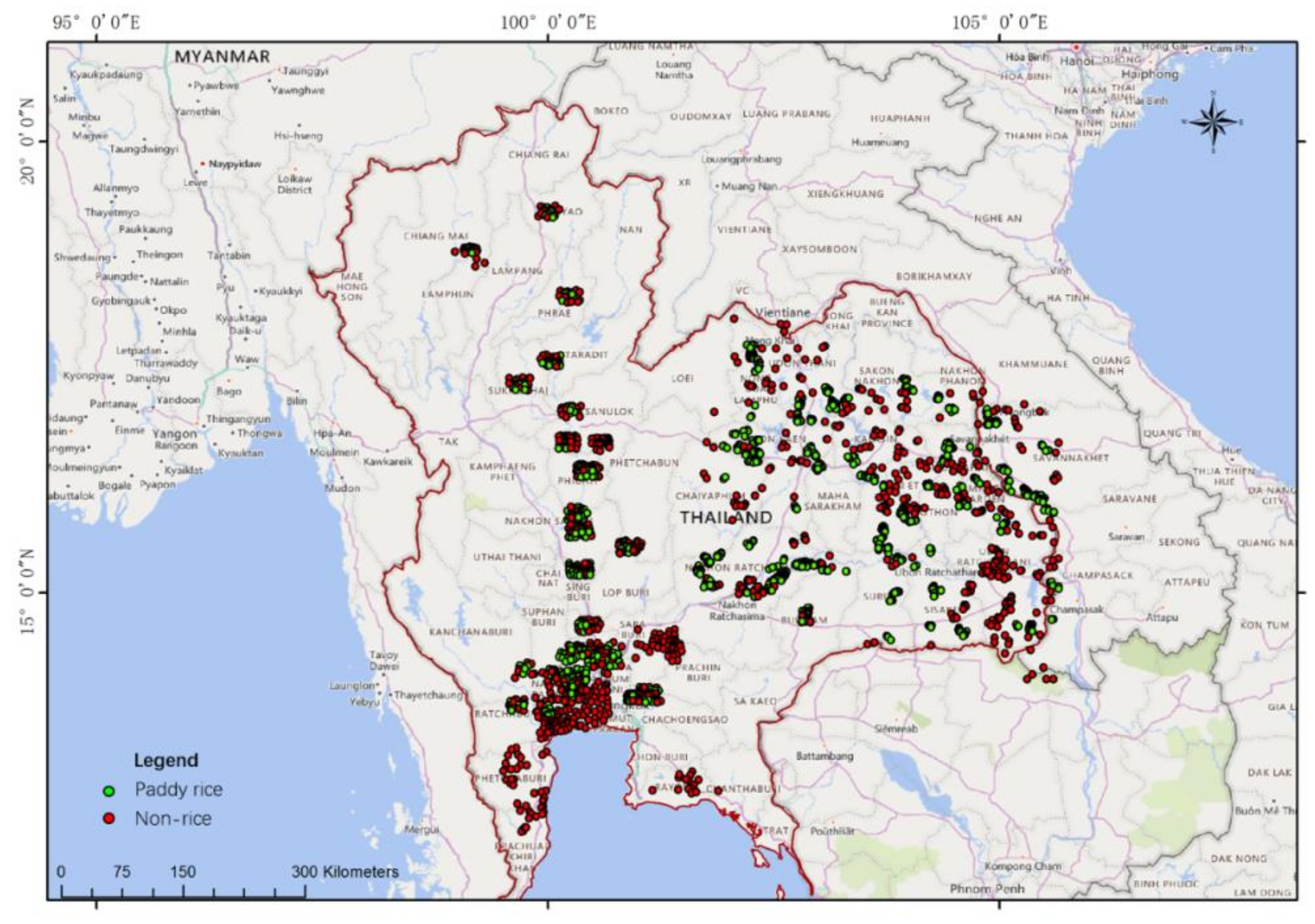
The difficulty of Thailand paddy rice mapping lies in two aspects. On one hand, the paddy rice in Thailand has various growth patterns. The σ 0 of the paddy rice fields may differ significantly from each other, so it is difficult to apply the classification methods that rely on the fixed relationship between phenology and time directly. On the other hand, the complicated distribution of croplands in Thailand caused by topography raise up with high requirement for the classification method. A reliable method that is able to identify small and scattered paddy rice fields and meanwhile be resistant to the sporadically distributed false alarms is demanded.
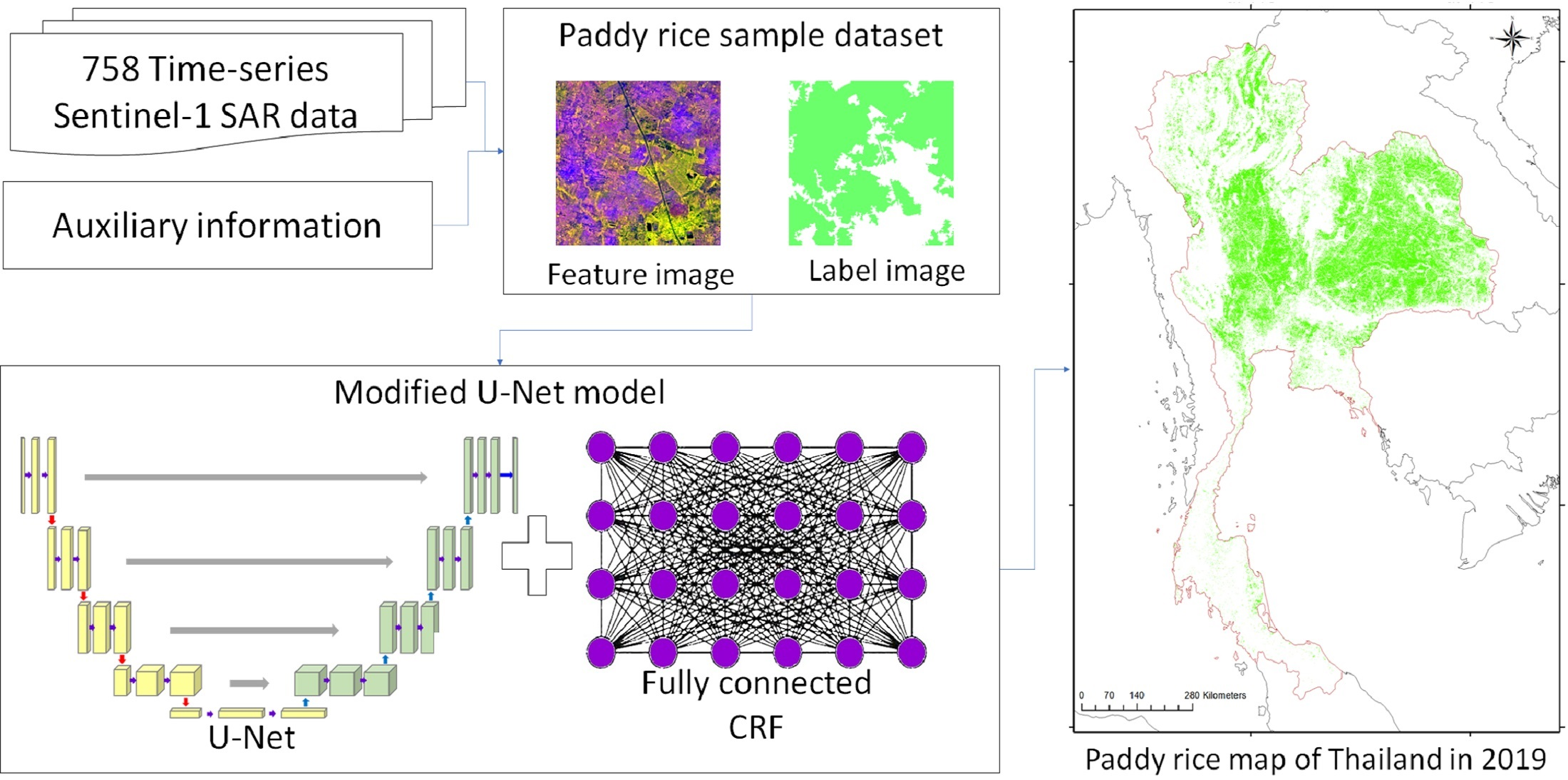
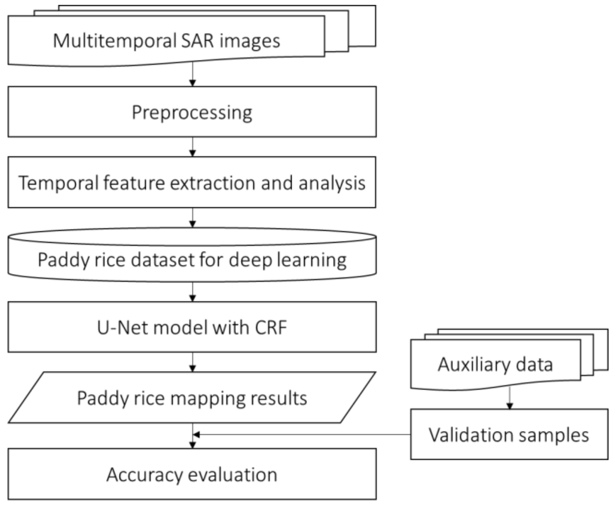
As a solution, this paper comes up with a paddy rice mapping scheme that is independent of the diverse cultivation patterns in Thailand and is capable of extracting small ground parcels despite the broken and irregular shapes. The flow chart of the proposed method is presented in Figure 5. First, the multitemporal Sentinel-1 images are preprocessed to get the calibrated σ 0 . The necessary preprocessing steps include coregistration, filtering, and geocoding. Then, features that capture the key information during growth are extracted from multitemporal SAR data. Considering the big data processing demands for the large area paddy rice mapping, the temporal statistic features of the time-series SAR data are computed and stacked as input to the deep learning network. To fully utilize the pixel-level semantics of the features, the U-Net model [51] is adopted to train the paddy rice prediction model, which uses the deconvolution layer instead of the pooling layer to construct the decoder structure and is capable to recover the spatial details of feature images. Finally, to improve the compactness and homogeneity of the classification result, the fully connected CRF is introduced to modify the U-Net model.

2.3.1. Preprocessing of Multitemporal SAR

The multitemporal Sentinel-1 images were preprocessed before the classification. The preprocessing was accomplished with ENVI Sarscape 5.2. First, the observations of the same frame were registered. Then, a multitemporal filter [56] was applied to each frame to suppress the speckle noise. Figure 6 compares the backscattering coefficient image of VH polarization ( σ V H 0 ) of a region of interest (ROI) area. It can be seen that the speckle noises are largely reduced after multitemporal filtering, and the boundaries between croplands and the other ground objects become clearer. After the filtering, the 30-m resolution Shuttle Radar Topography Mission (SRTM) DEM data were used for radiometric calibration and geocoding to extract σ V H 0 and σ V V 0 with a grid size of 20 m. Finally, the backscattering sequence models of σ V H 0 and σ V V 0 were generated, according to which the analysis of sowing and harvest patterns were carried out.

2.3.2. Extraction of Temporal Statistic Features

As illustrated above, the rice planting cycle in tropical countries such as Thailand can be very complex so that the general evolution models of σ 0 can hardly be summarized. Hence, three simple but effective temporal statistic features are defined from the dense time-series σ 0 images, which describe the most prominent SAR characteristics during paddy rice growth.
  • The temporal variance σ v a r 0
With the dramatic changes over leaves, stems, and fruits, the interactions between microwave radiation and crop canopy vary with time, leading to a large range of variations during plant growth and periodic changes in multiyear observations. By contrast, for non-agricultural objects, such as buildings, water, and forest, the change of σ 0 with time is less significant so that the temporal variance of σ 0 in annual SAR observations is the key to separate croplands from other land covers. The computation of σ v a r 0 can be expressed as follows, where n indicates the number of images, and σ m e a n 0 refers to the temporal average value of n images:
σ v a r 0 = 1 n i = 1 n σ t = i 0 σ m e a n 0 2
  • The temporal minimum σ m i n 0
Different from dryland crops, paddy rice has the transplanting stage when the plants are flooded underwater [57]. In this period, the σ 0 of paddy rice is only slightly higher than that of the water body, leading to distinct backscattering characteristic difference from other crops. Previous studies that targeted paddy rice mapping or crop classification methods have demonstrated the potential of the temporal behavior of σ 0 to distinguish paddy rice from other crops [54,55]. Therefore, in this study, the temporal minimum of σ 0 in each frame is computed with Equation (2) to determine whether the flooded period exists and to discriminates rice from other crops:
σ m i n 0 = min t = 1 , 2 n σ t 0
  • The temporal maximum σ m a x 0
Influenced by factors such as monsoons, floods, aquatic plants, and so on, some water bodies can also display seasonal backscattering changes. If the identification of paddy rice only relies on σ m i n 0 , false alarms might occur because of the misclassification of water bodies. Since σ 0 of paddy rice rises substantially in vegetative and reproductive stages, the temporal maximum of σ 0 in SAR sequences is useful to avoid the influence of water. The computation of σ m a x 0 can be expressed as:
σ m a x 0 = max t = 1 , 2 n σ t 0
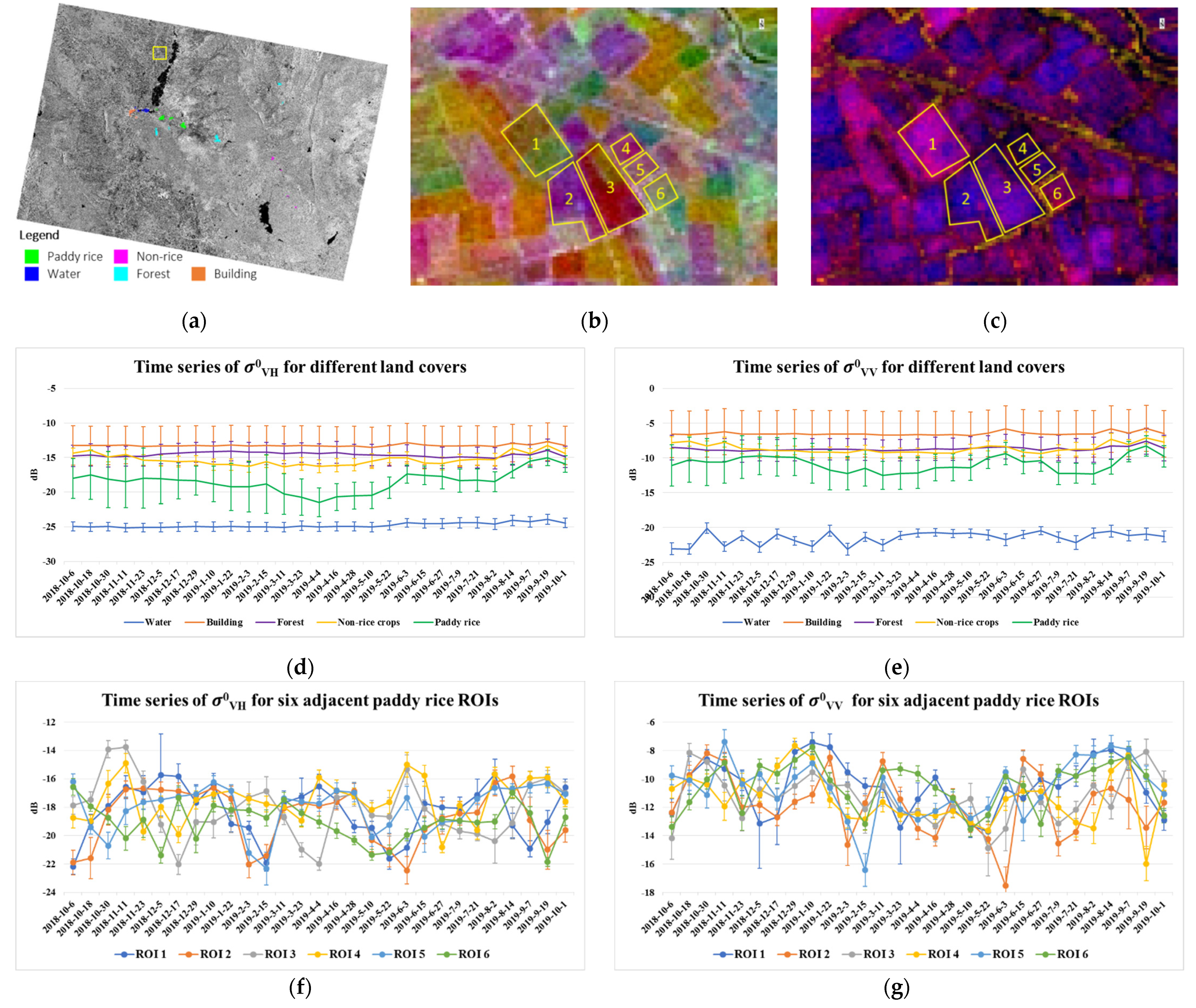
To illustrate the potential of the temporal features, Figure 7 depicts the mean σ V H 0 and σ V V 0 curves of several regions of interest (ROIs), whose locations are shown in Figure 7a. The error bars represent the standard deviations of each ROI. Firstly, the mean σ V H 0 and σ V V 0 curves of different land covers are compared in Figure 7d,e. Compared to other land covers, such as buildings, non-rice crop, and forest, σ V H 0 and σ V V 0 curves of paddy rice both show obvious fluctuations, especially from March to October 2019. Meanwhile, from 6 October 2018 to 4 April 2018, the standard deviations of paddy rice were no less than 2 dB and even reached to 4.32 dB (in VH polarization) on 23 November 2018. Other land covers, such as buildings and non-rice crops, also have higher standard deviations, especially in VV polarizations. As a result, in both VH and VV polarizations, the σ 0 values of paddy rice and other land covers overlap with each other, which are likely to cause misidentifications if using traditional thresholding methods.
To make further inspection on the diverse paddy rice cultivation patterns, six adjacent paddy rice parcels were selected, whose location is indicated by the yellow box of Figure 7a. Figure 7b shows the false-color image composited by σ V H 0 on 11 March, 22 May, and 14 August 2019, whereas Figure 7c displays the false-color image of σ m a x 0 , σ m i n 0 , and σ v a r 0 in VH polarization. In Figure 7b, these ROIs display different colors, indicating different backscattering intensities in VH polarization on 11 March, 22 May, and 14 August. In other words, even though spatially close to each other, these ROIs had different cultivation practices, which is also validated by the mean σ V H 0 and σ V V 0 curves shown in Figure 7e,f. For ROI 1 and ROI 2, triple-season paddy rice was cultivated during the observing period: the first-season lasted from October to February, the second-season lasted from February to May, and the final season lasted from May to September. For ROI 3, two complete paddy rice growing seasons can be observed: the first one was from December to April, and the second one was from April to August. As for ROI 4, only one complete paddy rice growing season is observed, which lasted from December to June. ROI 5 had a similar first two seasons as ROI 1 and ROI 2, but the third paddy rice season was much longer. ROI 6 also cultivated double-season paddy rice, but the growing cycle is different from ROI 3: the first-season lasted from December to May, and the second one was from May to September. As demonstrated by Figure 7b,f,g, the diverse paddy rice cultivation patterns in Thailand was exactly the most notable characteristic in tropical areas. In contrast, despite the various cultivation practices, these ROIs display similar hues in Figure 7c (purple, magenta, and red), which indicates that the temporal features are capable to capture the key information of paddy rice fields even under different growing patterns.
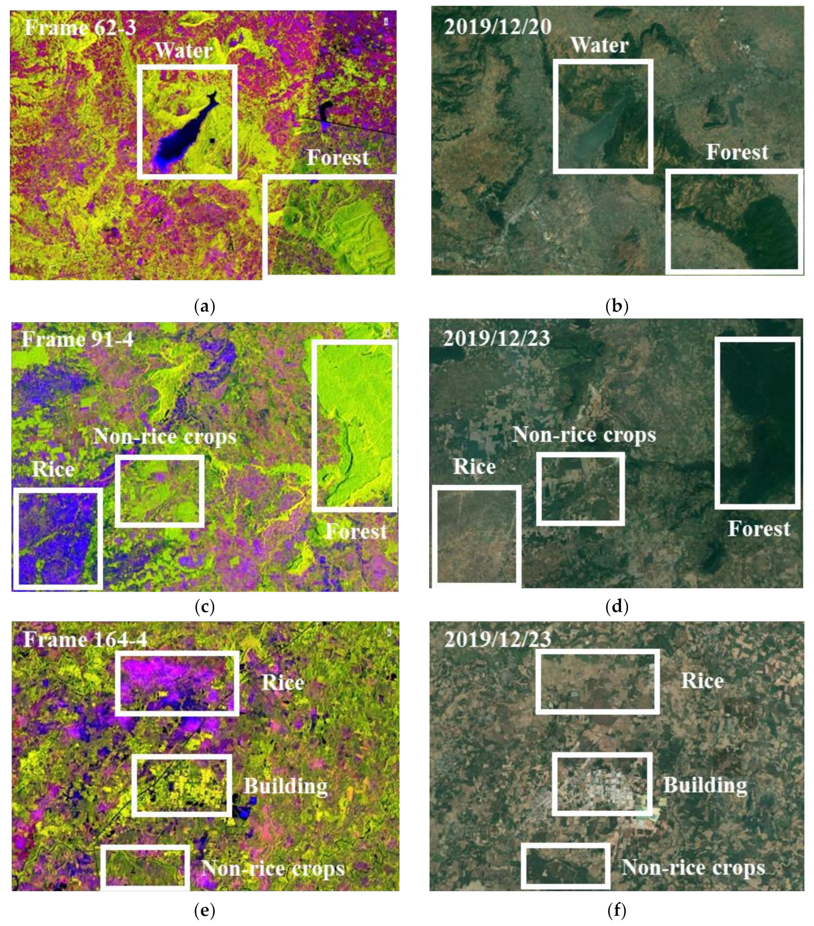
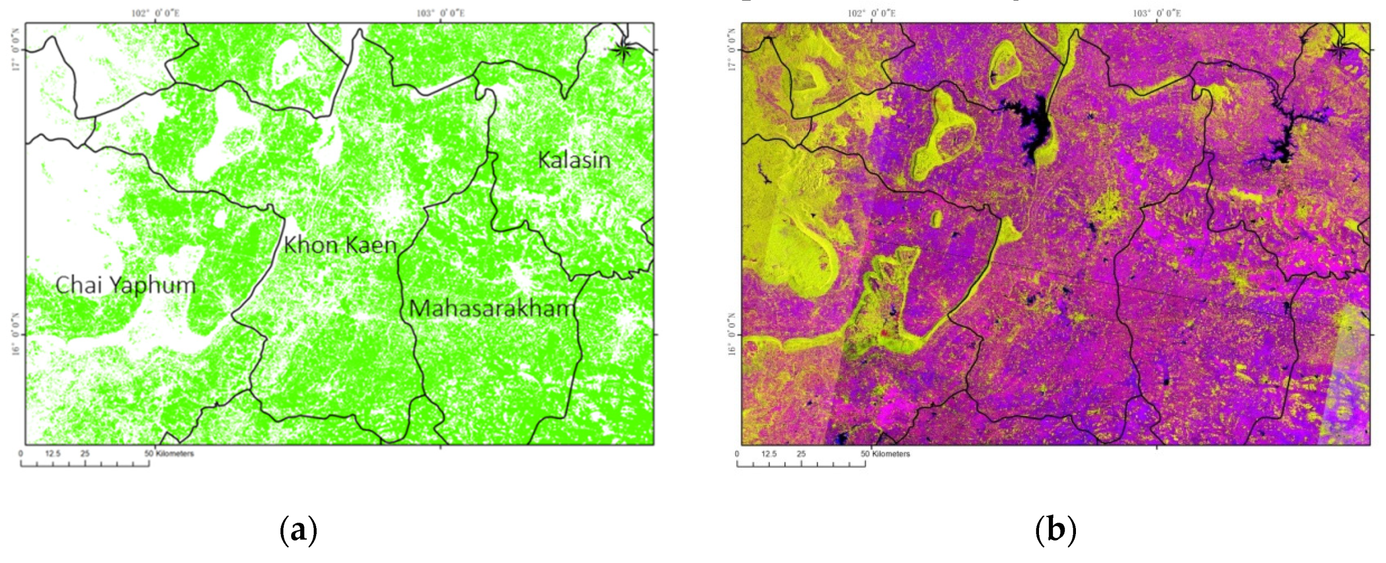
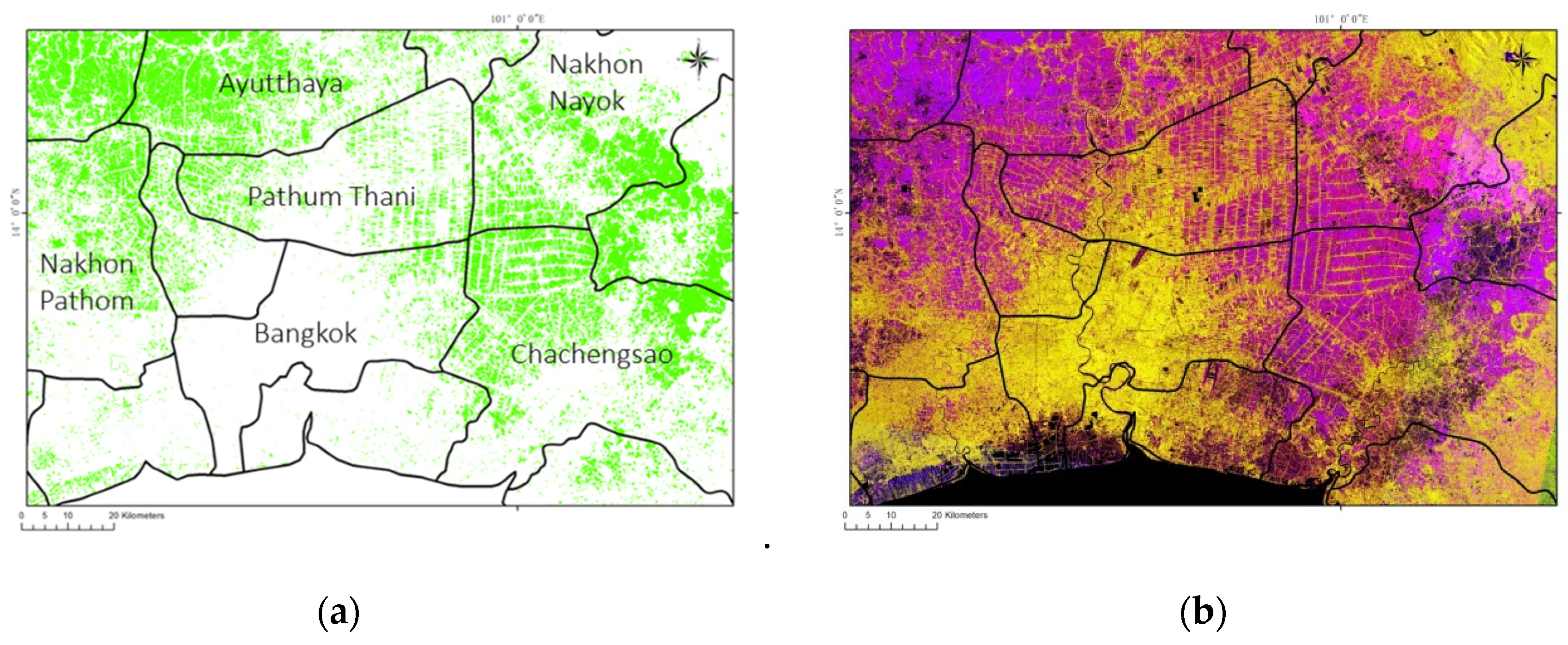
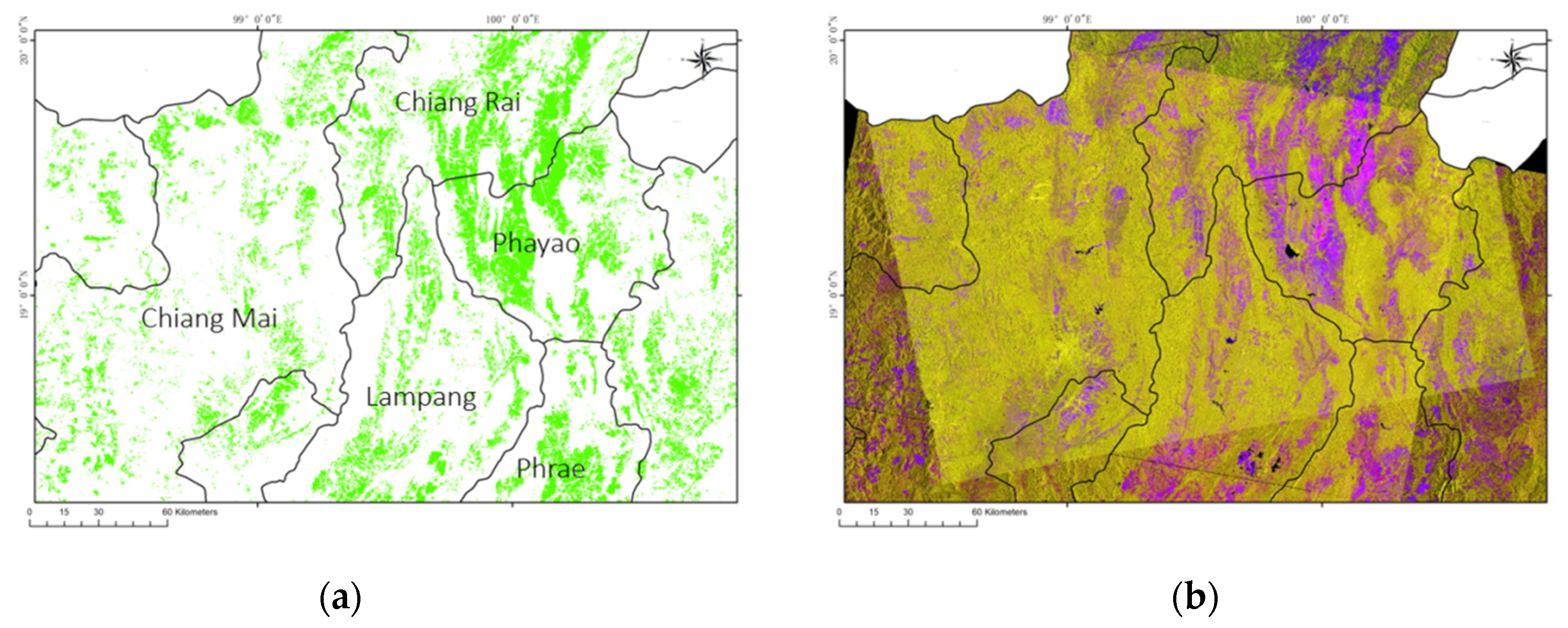
Furthermore, Figure 8 gives the false-color images and corresponding Google Earth optical images of typical land covers. The uniqueness of paddy rice lies in its high values of σ v a r 0 and σ m a x 0 and meanwhile with a low value of σ m i n 0 , which usually leads to magenta in the false-color image. Since the hue is affected by the relative intensity of σ v a r 0 and σ m a x 0 compared to the whole frame, sometimes paddy rice fields also appear as red or dark blue. Compared to paddy rice, the values of σ m i n 0 of other non-rice crops are much higher. In other words, the green component is higher, resulting in green, dark yellow, or brown in the RGB image. Water bodies appear as dark regions because of low σ m a x 0 , σ m i n 0 , and σ v a r 0 . Land covers with stable backscattering intensities, such as buildings and forest, generally have very low σ v a r 0 and high σ m i n 0 ; as a result, these land covers appear yellow or green in the false-color image.
Previous studies have demonstrated the correlation between paddy rice parameters and cross-polarizations (HV or VH) was slightly higher than that of VV polarization in C-band and performed better in paddy rice identification [52,55,58,59,60]. The VH polarization is mainly affected by the volume scattering mechanism of the canopy, whereas VV polarization is affected by the double-bounce and surface scattering mechanisms of the canopy and ground surface. The disappearance of standing water, the reflection changes between stems and ground surfaces, and the vertical structure variations of paddy rice during the vegetation stage contribute comprehensively to VV polarization. It is more difficult to summarize the growth pattern of paddy rice using VV polarization, which is also confirmed by the comparison of Figure 7f,g. Therefore, in this study, only VH polarization is used for paddy rice mapping. 
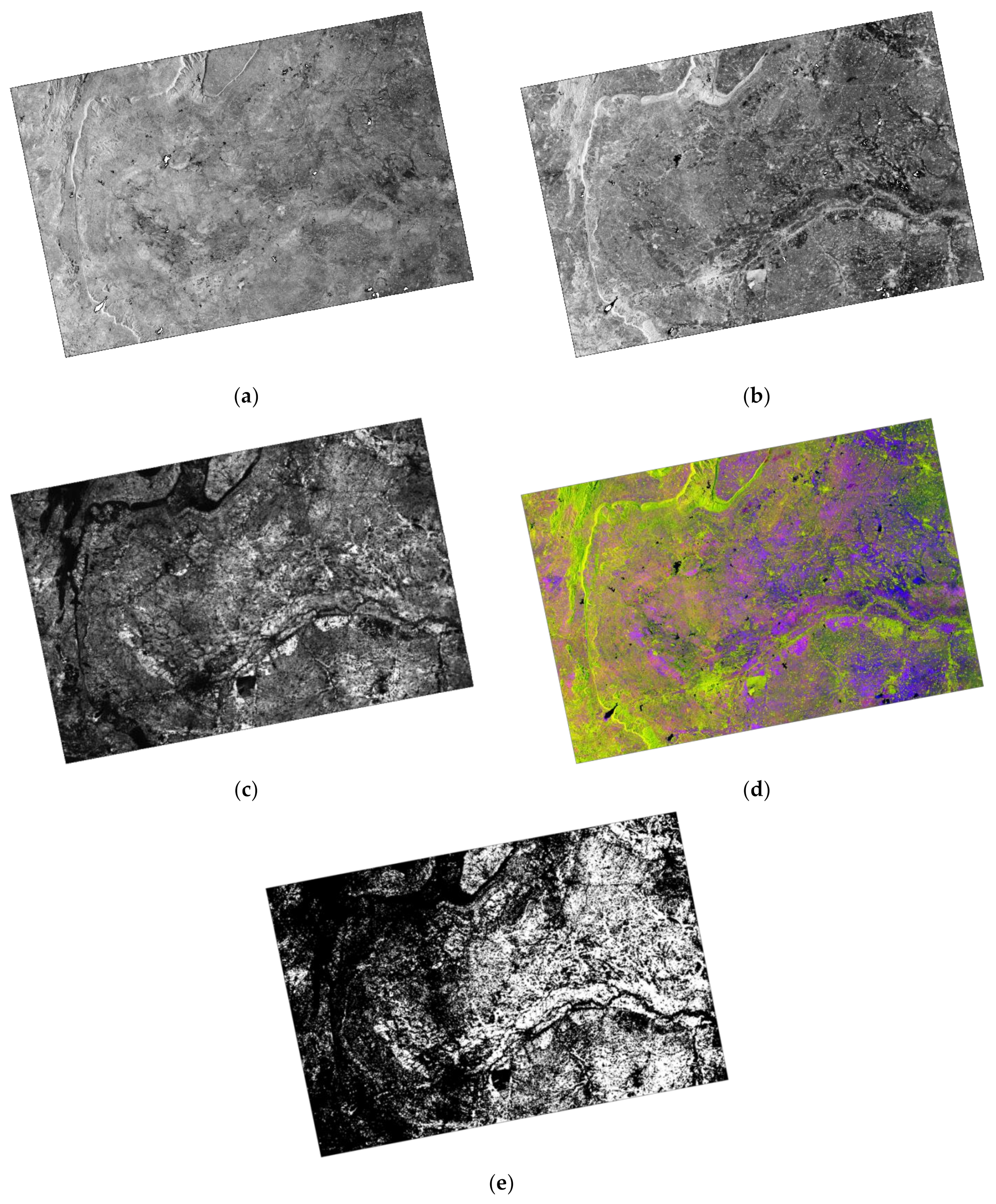
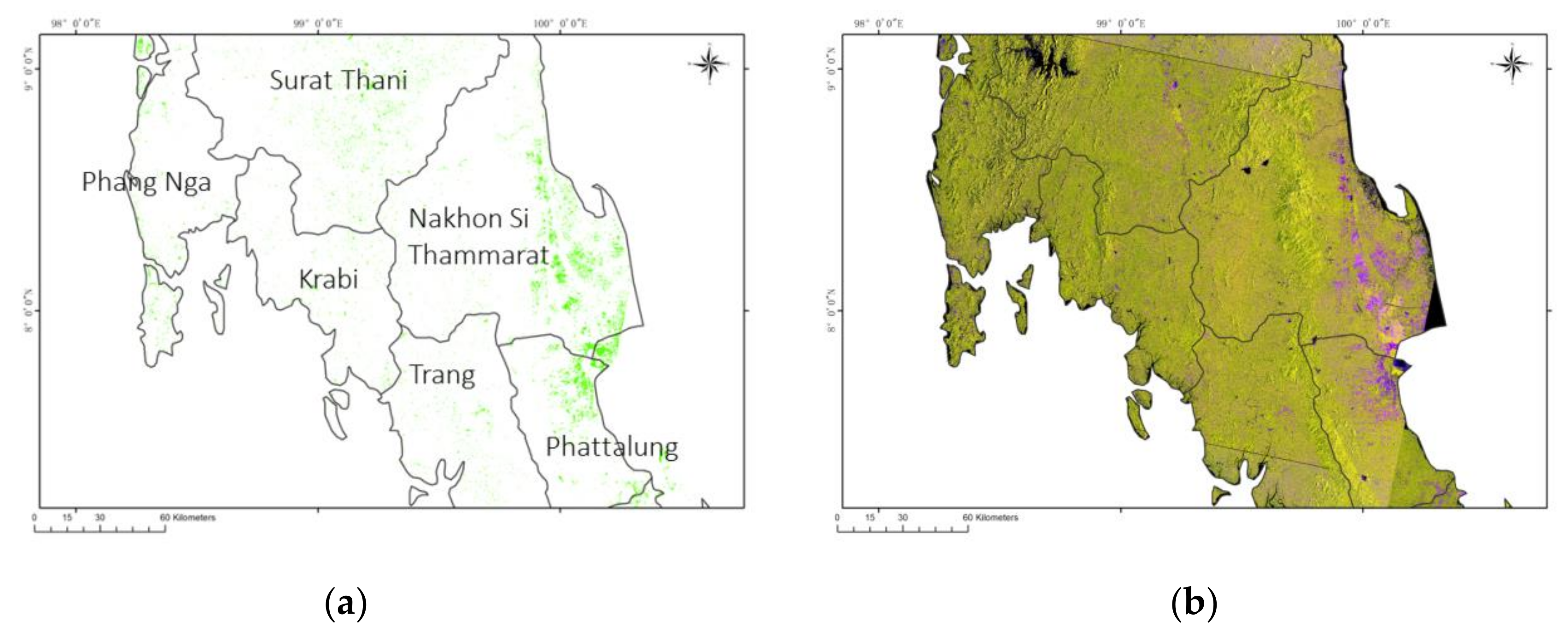
Figure 9 displays the temporal features of VH polarization extracted from frame 99-16. The false-color image shown in Figure 9d is taken as the training dataset, and the corresponding label image is displayed in Figure 9e. 
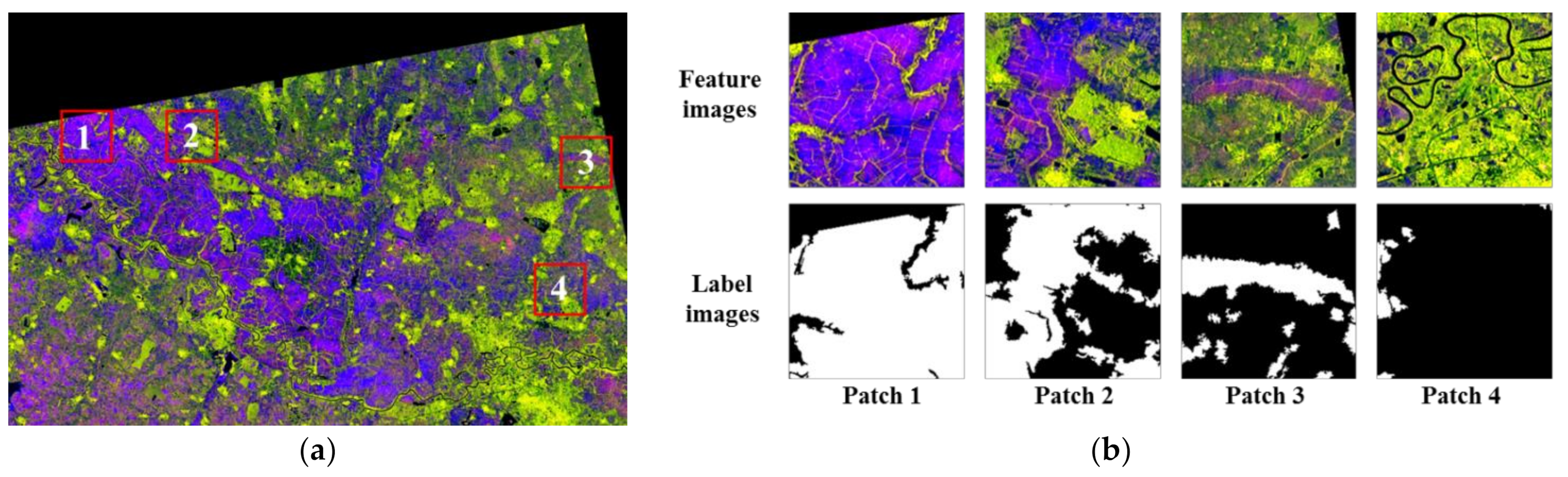
Figure 10 shows some examples of the training patches for the paddy rice mapping model, which were randomly selected from the training dataset. When the model is trained, the false-color images of all other frames were extracted and constitute the classification dataset that to be predicted. 
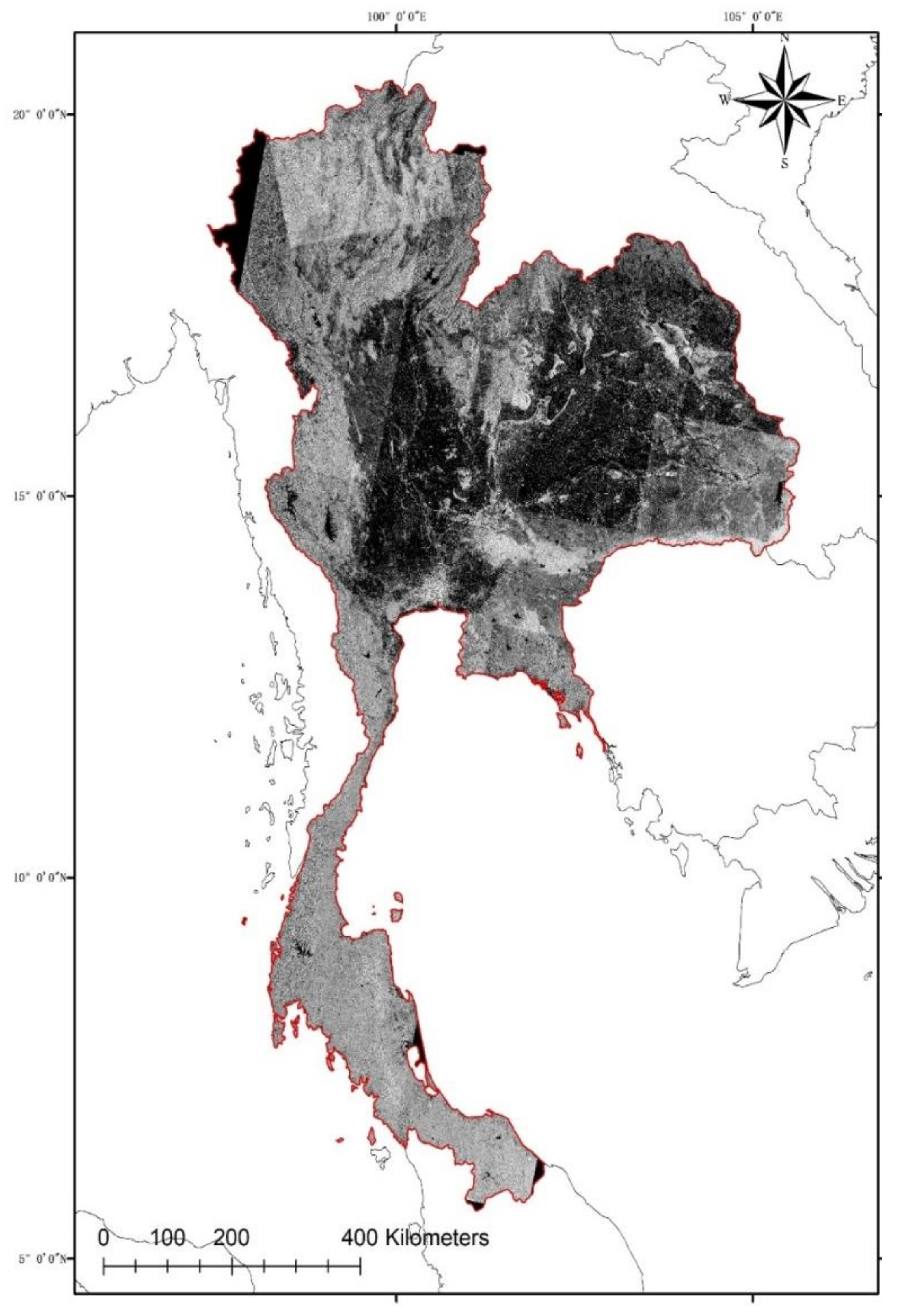
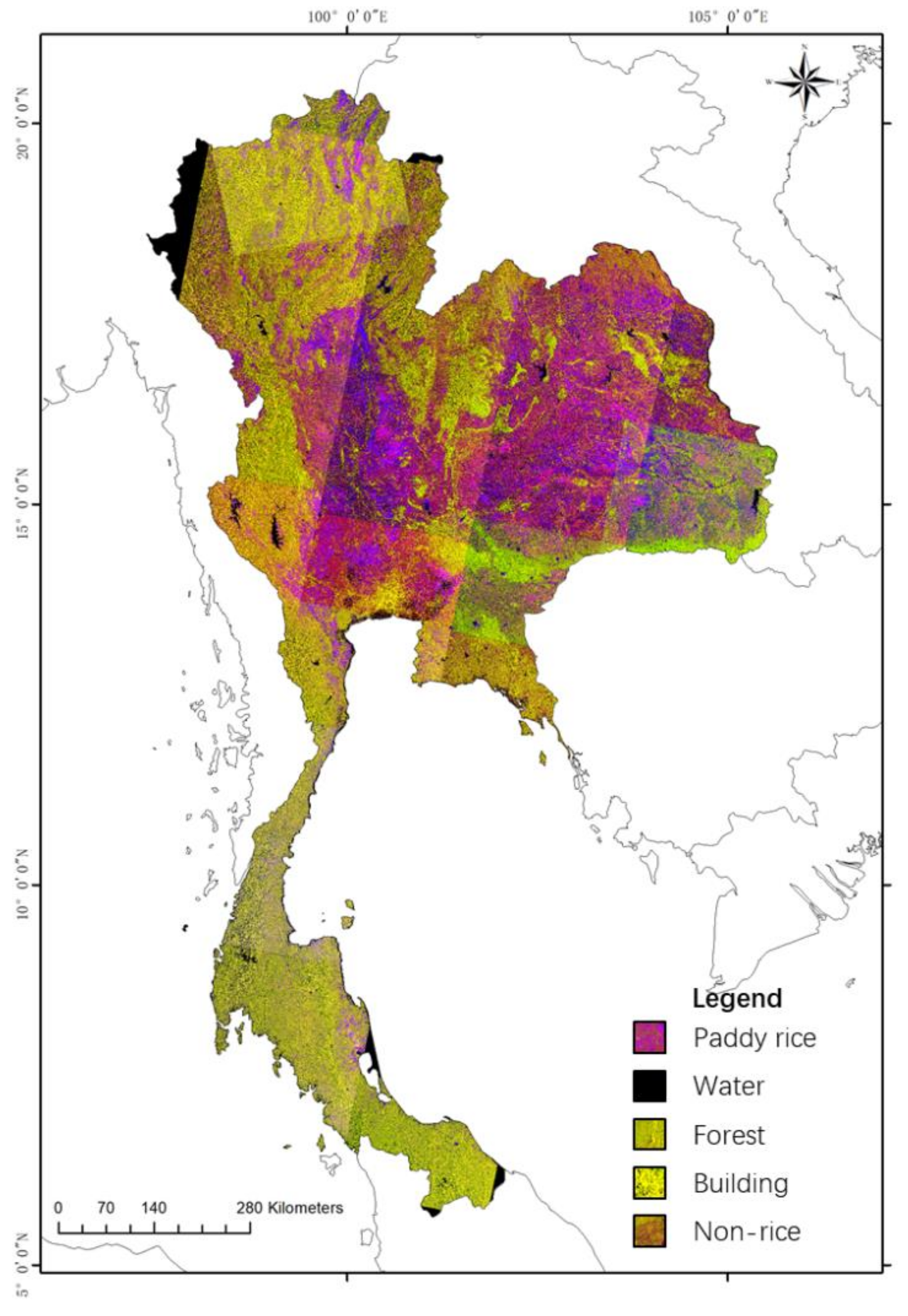
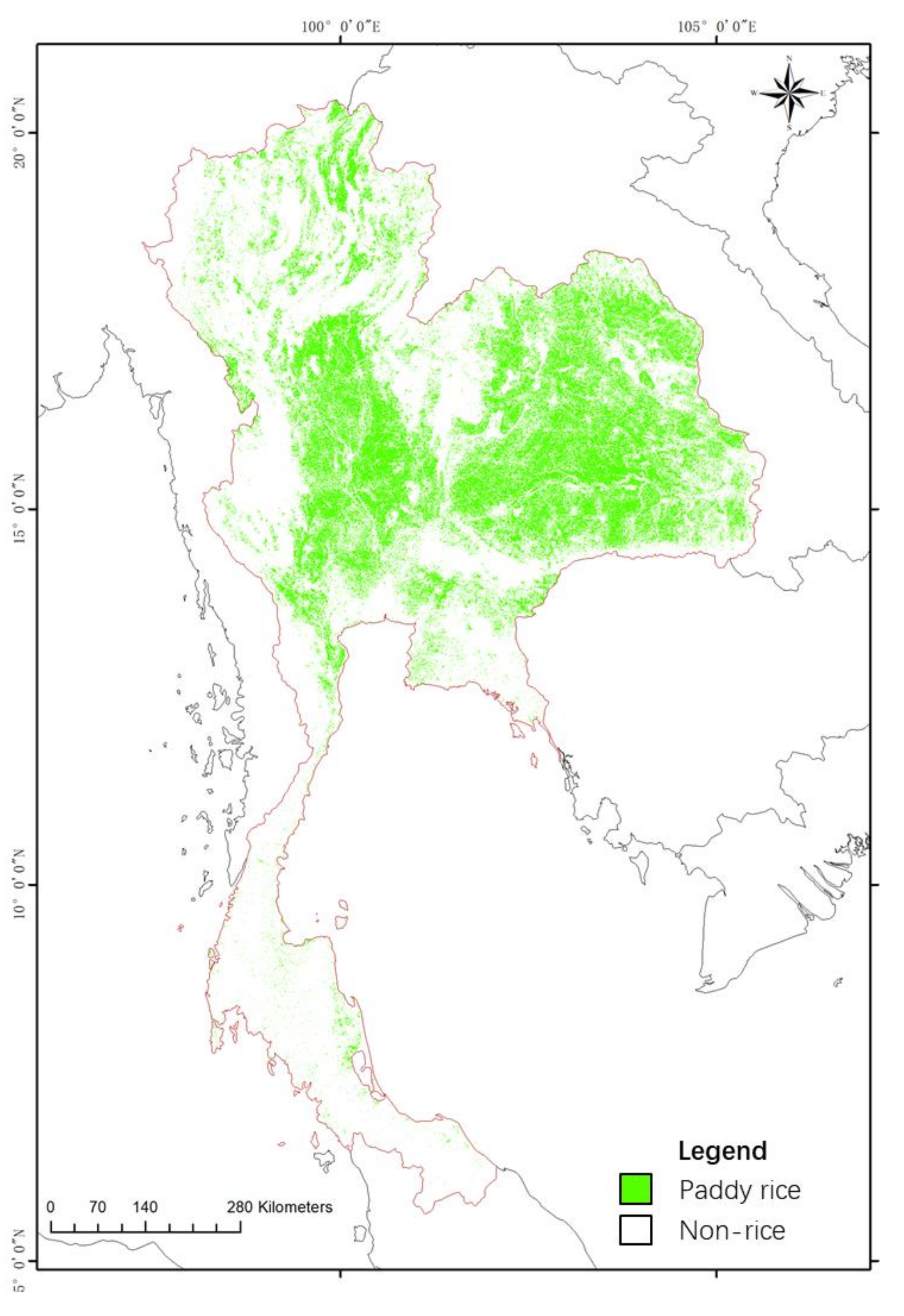
Figure 11 shows the false-color temporal feature images of whole Thailand, which is mosaicked and harmonized to get consistent hues. The automatic mosaicking was accomplished by ENVI 5.3. In overlapping regions, the frames on the west and north side was in front of the ones on the east and south side.

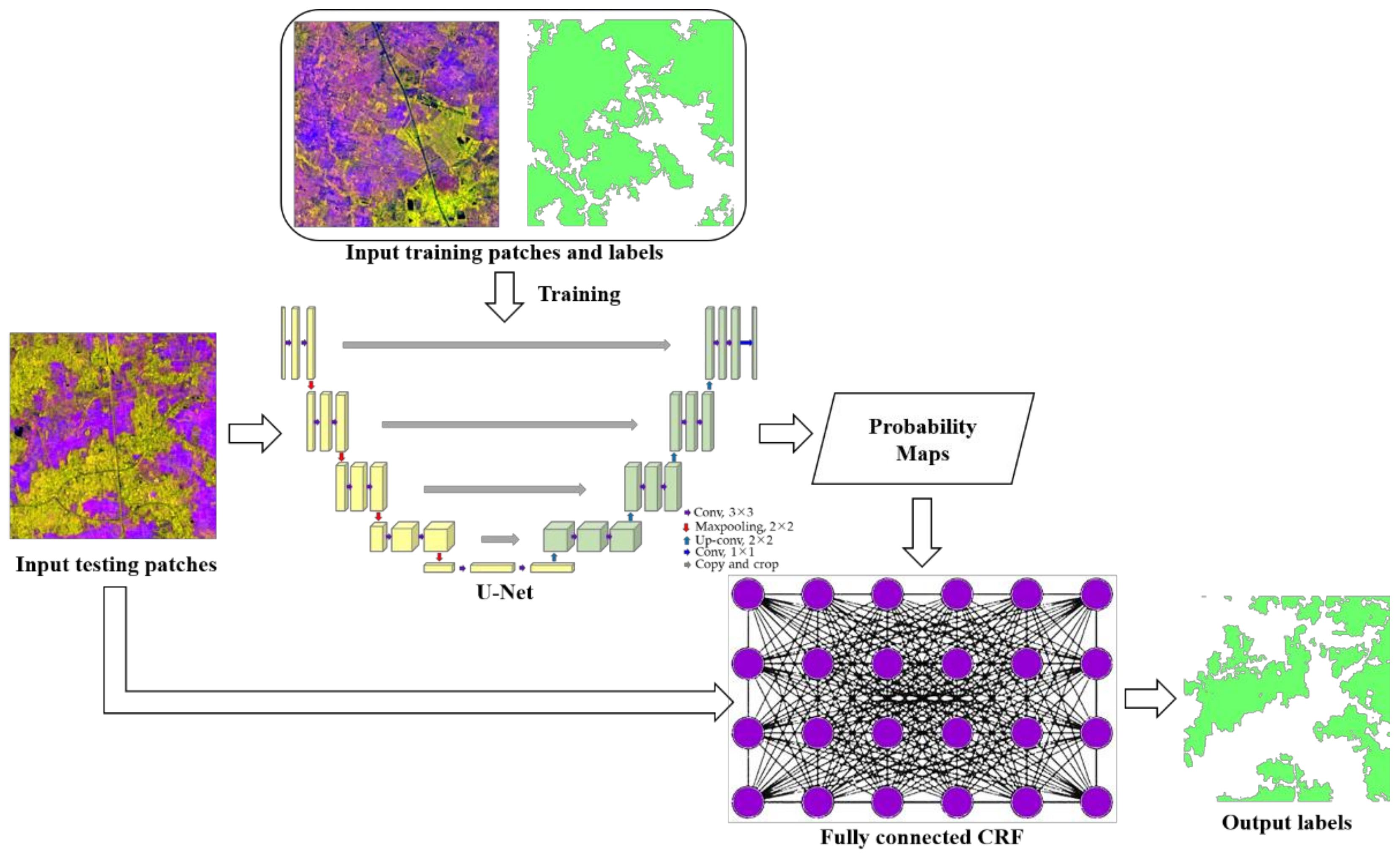
2.3.3. The Modified U-Net Model for Paddy Rice Mapping

In this study, the U-Net model was utilized to accomplish the paddy rice mapping task. The fully connected CRF module was introduced to modify the U-Net model to improve the performance of paddy rice extraction in Thailand. The flowchart of the proposed model is shown in Figure 12.
  • The basic structure of U-Net
The classical CNN structure can only tell whether a certain class exists in the input image but cannot predict the semantic information of each pixel. In contrast, FCN outputs a pixel-by-pixel semantic label image corresponding to the input image by replacing the fully connected layers of CNN with the convolution layers so that the output classification map maintains the same resolution as the input images [61]. In this study, we applied the U-Net model to extract a high-resolution paddy rice map of Thailand. As an improved FCN model, U-Net extracts high-level semantic features while maintaining the spatial details of the input image [
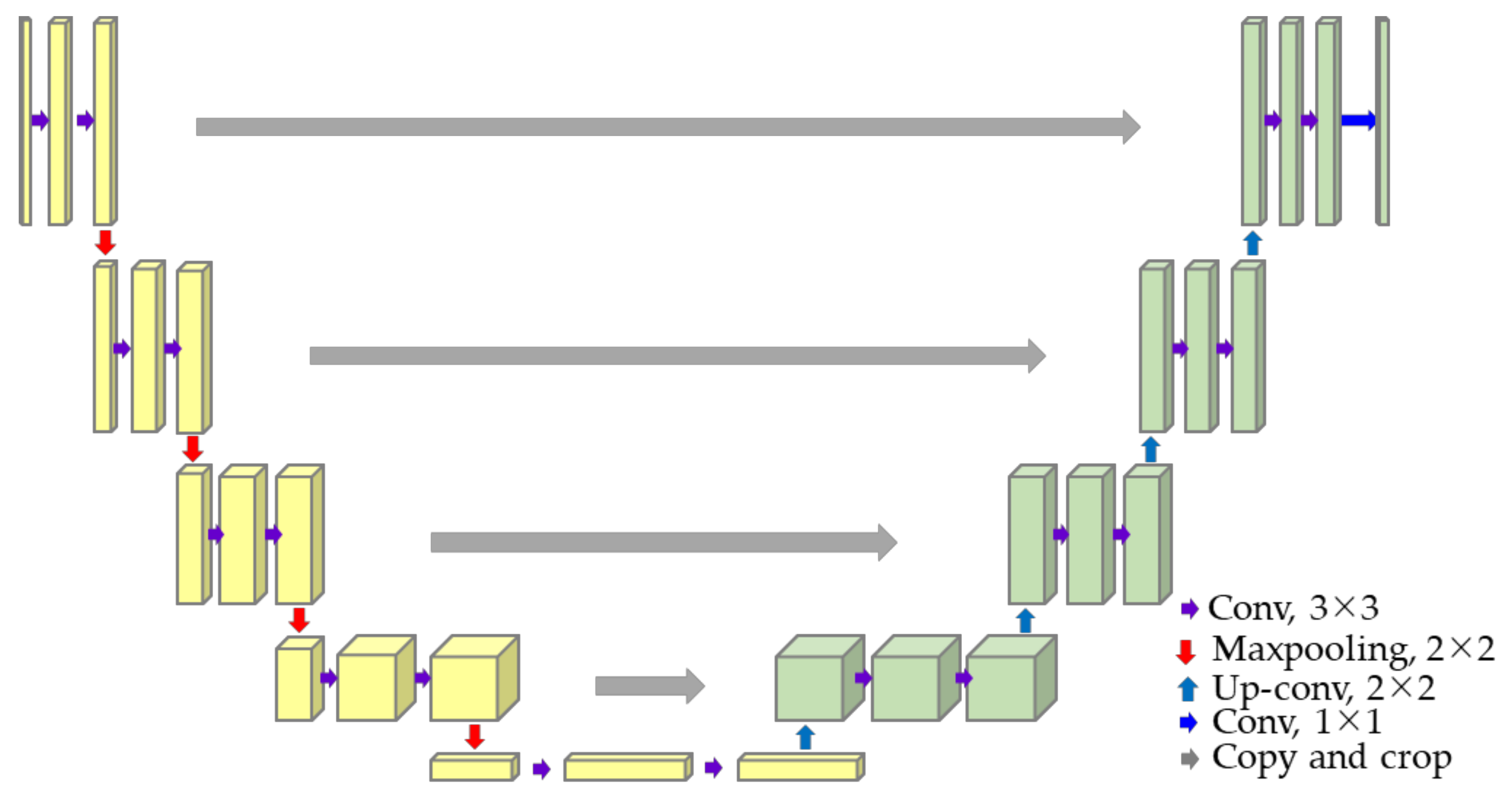
51]. The structure of U-Net is displayed in Figure 13. The model contains 23 convolution layers in total. The encoder part is consisted of five down-sampling units, where each unit is composed of two 3 × 3 convolution layers and a 2 × 2 max-pooling layer. The decoder contains four up-sampling units, where each unit is composed of two 3 × 3 convolution layers and a 2 × 2 deconvolution layer. Finally, the feature vector of the last up-sampling unit is converted to probability maps by a 1 × 1 convolution layer, where the dimension of probability maps equals the number of classes, and the pixel value of each map represents the probability that the pixel belongs to the corresponding class.
  • The Batch Normalization (BN) layer
To improve the training efficiency, in this paper, we introduce the Batch Normalization (BN) layer [62] into the original U-Net model. Before each convolution layer, a BN layer is applied to the input of the activation function (such as a sigmoid function or a ReLU function) to ensure that the input data follows the same distribution whose mean is 0 and variance is 1. The formula for BN can be expressed as:
BN x i = γ x i μ B σ B 2 + ϵ + β
where x i represents the input of mini-batch i , μ B and σ B 2 represent the mean and variance in the mini-batch, γ and β are scale and bias parameters that need to be trained, and ϵ is a smooth item to assure that the denominator will not be zero.
  • The fully connected CRF module
As mentioned above, the paddy rice plots in Thailand are small, fragmented, and with unclear edges, which may cause broken plots and rough boundaries in the classification results. To solve this problem, this study introduces fully connected CRF [53] to improve the output of the U-Net model.
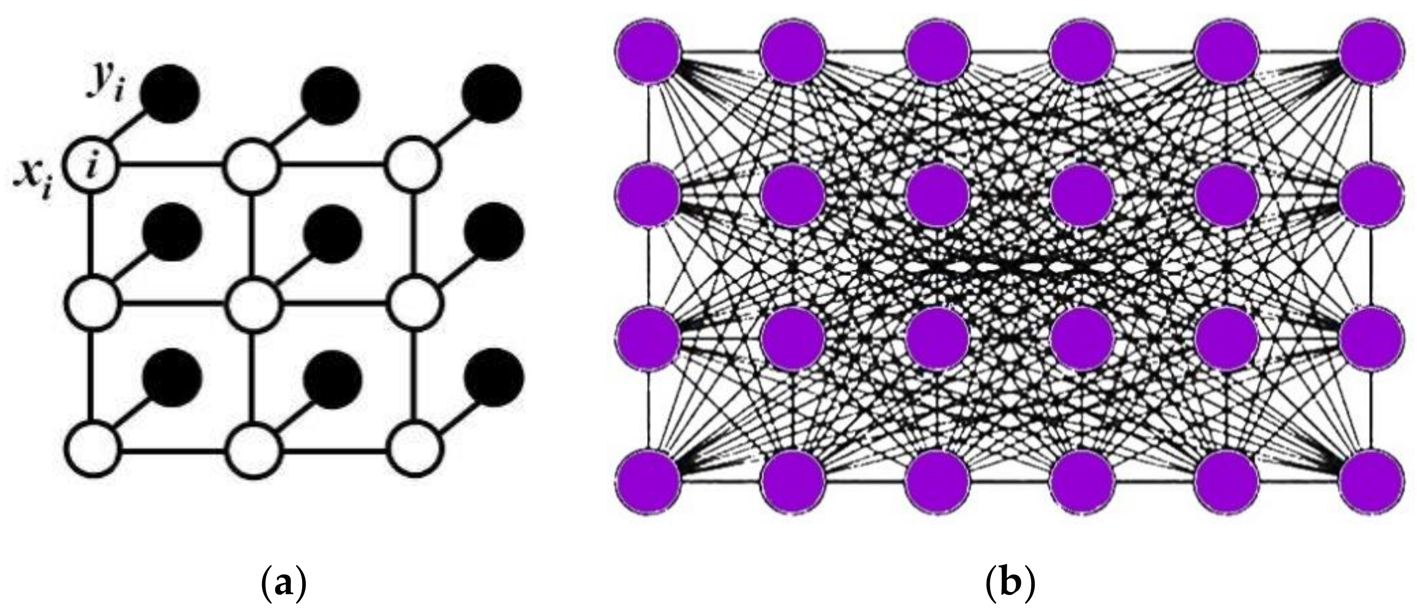
CRF is essentially an undirected graph model based on Markov Random Fields (MRF), which can describe the dependence or spatial correlation between pixels [63]. As shown in Figure 14a, each node in CRF is composed of the label x i and the value y i of pixel i , and the edge between two nodes denotes the relationship between two corresponding pixels. Through the spatial correlation between nearby pixels, misidentifications will be effectively eliminated, leading to consistent classification results. As a modification of CRF, fully connected CRF links all the pixels in the image to avoid over-smoothing caused by spatial modeling in a limited neighborhood, as shown in Figure 14b. The pixel value y i and the spatial distances between pixel i and others are both considered to modify the label x i . The energy function of fully connected CRF can be expressed by:
E x = i Ψ u x i + i < j Ψ p x i , x j
Ψ p x i , x j = u x i , x j m = 1 M ϖ m k G m f i , f j
where Ψ u x i is the unary potential energy provided by x i , which is the probability map generated by the softmax function of U-Net model; Ψ p x i , x j is the binary potential energy provided by adjacent pixels i and j ; u x i , x j is a label compatibility function; ϖ m is the linear combination weight; k G m is the Gaussian kernel function that considers the spatial similarity and pixel value similarity comprehensively and assigns the same semantic label to similar pixels; and f i and f j are feature vectors of pixels i and j in an arbitrary feature space. The detailed expressions of k G m were given in [53], which presented a fast inference algorithm of applying fully connected CRF. The probability maps acquired by U-Net as well as the original feature images are used to calculate the energy function of fully connected CRF, which is minimized iteratively to obtain the final paddy rice mapping results.

2.3.4. Accuracy Assessment and Validation Data

Auxiliary data, including Google Earth optical image and Sentinel-2 optical data, were also acquired to collect the validation samples of accuracy evaluation. The validation samples were divided into “paddy rice” and “non-rice” according to visual interpretation, which includes 925 paddy rice plots and 1096 non-rice plots (including non-rice crops, water, urban, and forest), as given in Table 2. The validation sample plots were randomly distributed across the main paddy rice production regions, as presented in Figure 15. These plots were utilized for the accuracy assessment of paddy rice mapping. Considering paddy rice as “positive” and non-rice as “negative,” four indexes can be calculated to evaluate the performance of the proposed model:
A c c u r a c y = T P + T N T P + T N + F P + F N
P r e c i s i o n = T P T P + F P
R e c a l l = T P T P + F N
K a p p a = A c c u r a c y p e 1 p e
  p e = T P + F N × T P + F P + T N + F P × T N + F N T P + T N + F P + F N 2
where T P , T N , F P , and F N refer to true-positive, true-negative, false-positive, and false-negative predictions; A c c u r a c y evaluates the overall prediction performance; P r e c i s i o n refers to the capability of extracting paddy rice correctly; R e c a l l describes to the omission level of paddy rice; and K a p p a refers to Kappa coefficient, which indicates the overall consistency of prediction and ground truth.

3. Results

3.1. Training Details of the Proposed Paddy Rice Mapping Method

The details of the U-Net model training are given in Table 3. The kernel function size, stride size, activation functions of the convolution layers, pooling layers, and deconvolution layers were the same as the original model in [51]. The padding strategy was applied to make sure that the output has the same size as the input. The padding value was set to 1. The model was trained using frame 99-16 as illustrated in Section 2.2.2 and Section 2.3.2. The temporal features of all other data frames were extracted, and the false-color image patches were generated for paddy rice recognition. After the predictions, all the patches were stitched together to generate the paddy rice map of Thailand. If the predictions of the overlapping areas in different frames were inconsistent, the result takes the union of the predictions to avoid misidentification.

3.2. Paddy Rice Mapping Results and Accuracy Assessment

Figure 16 displays the paddy rice mapping result of Thailand in 2019. As mentioned in Section 2.1, the distributions of paddy rice are influenced by the complex terrains as well as the production conditions. Affected by topographical factors, the paddy rice fields are usually small and scattered.
Figure 17, Figure 18, Figure 19 and Figure 20 display some detailed results and the false-color images of the representative paddy rice production regions. Figure 17 shows the partial paddy rice mapping result in northeast region. Located at the central part of the Khorat Plateau, Khon Kaen, Mahasarakham, and Kalasin all have distinct dry and rainy seasons. The rain-fed, single-season rice is the main production in these areas because rain is the main water source. As reflected by Figure 17, the total paddy rice cultivation area is very large, but the paddy rice plots are small and have irregular shapes. Figure 18 shows the paddy rice mapping results around Bangkok, the capital of the nation. In contrast to the Northeast region, the central plain has a higher urbanization level and more advanced irrigation facilities. Located near the most prosperous city in the country, the fields in the suburbs of Bangkok, Chachengsao, Pathum Thani, and Nakhon Nayok are well organized. The paddy rice fields in Figure 18b display clear boundaries, which indicate regular land-use allocation. Figure 19 shows the results of Chiang Mai and Chiang Rai, which are representative in northern region. The distribution of paddy rice is concentrated at the valleys, which is in good consistency with the false-color image of the temporal features. Besides, even small and discrete paddy rice plots were successfully extracted by the proposed method. Figure 20 depicts the results in southern Thailand, where paddy rice only accounts for a small portion and the paddy rice plots are relatively small compared to other regions.
With the validation samples given in Table 2 and Figure 15, the paddy rice mapping accuracy is evaluated as listed in Table 4. According to Equations (7) to (10), A c c u r a c y is the ratio of correctly discriminated pixel number to the total validation sample number, and R e c a l l is the ratio of the correctly discriminated paddy rice pixel number to the total paddy rice pixel number. The fact that these parameters surpass 90% and 95% indicates that most pixels in the validation dataset are successfully identified; meanwhile, the omission rate of paddy rice is low. P r e c i s i o n is the proportion of true paddy rice pixels in all detected paddy rice pixels. For the proposed method, P r e c i s i o n reaches 87%, which illustrates that the false alarms can be effectively eliminated by the proposed method. For the classification task, K a p p a evaluates whether the predicted result is consistent with the ground truth and is influenced by the degree of imbalance in the classification result. In this study, K a p p a is 0.8262, which indicates that no significant imbalance exists in the predicted paddy rice map. The paddy rice mapping result matches well with the validation samples, which demonstrates that the proposed method is capable of grabbing key information and portrays accurate paddy rice distribution in the large tropical areas under various topographies and cultivation conditions.

3.3. Comparisons to the Official Statistics

Figure 21 compares the predicted paddy rice area and the statistics of paddy rice cultivation area released by OAE [64]. According to the statistics of agricultural land utilization in 2019, the total area for agricultural use was about 238,803.92 km2 (149,252,451 Rai, where 1 Rai = 0.0016 thousand km2), among which paddy rice accounted for about 46.04% and was 109,955.82 km2, approximately. The total predicted paddy rice area of the proposed method was approximately 136,587.16 km2, which was overestimated by 24.22% compared to the statistics of OAE.
To investigate possible reasons for this overestimation, we further calculated the proportion of predicted paddy rice area to all croplands using another remote sensing LULC product. The FROM-GLC global LULC product (2017v1) [19] was chosen to make a direct comparison to our paddy rice map after resampling the 10-m resolution LULC product into 20-m resolution. The comparison was carried out under the assumption that the total cropland area had not changed significantly in two years, which was supported by the statistics of OAE (the agricultural land from 2017 to 2019 were almost the same [64,65,66]). The total cropland of Thailand extracted by FROM-GLC was 311,974.23 km2, and the ratio of predicted paddy rice area to all croplands in FROM-GLC LULC was 47.55%, which was close to the paddy rice proportion of OAE statistics.
Compared to the official statistics, the paddy rice areas have been overestimated in our paddy rice mapping result and the FROM-GLC LULC product. A possible reason was that the statistical cycle was not strictly consistent with data acquisition periods. In this study, no matter when the field was planted, all the fields that were cultivated with paddy rice were labeled by the proposed method. However, some paddy rice fields might have contributed to the last year by OAE because it computed the statistical data according to the planting seasons. Besides, the statistical data itself may also contain errors. OAE mainly considered well-organized, single-season and double-season paddy rice in all the statistics so that some casual and irregular planting practices by individual households were inevitably ignored. Considering the data acquisition conditions and statistical errors, the difference between the extracted paddy rice map and the official statistics was understandable.

3.4. Comparisons to Other Classification Methods

3.4.1. Experimental Area

To demonstrate the effectiveness of the proposed scheme and to evaluate how different methods perform in paddy rice discrimination, we used frame 62-4 as an example to make direct comparisons to other two methods. Frame 62-4 contains typical land covers, including paddy rice, non-rice crops, water, urban, and forest areas, whose location is shown in Figure 22a. It contains 173 paddy rice validation plots (575,307 pixels) and 285 non-rice validation plots (588,658 pixels), which make good support to a reliable accuracy assessment, as shown in Figure 22b.

3.4.2. Other Classification Methods for Comparison

  • Support Vector Machine (SVM)
To illustrate the performance of the modified U-Net model designed in this study, SVM was taken as the baseline. It is one of the most widely applied methods for the classification of remote sensing images [67], which projects the non-linear feature space into linear feature space in a higher dimension and acquires accurate classification model. The same input feature image (false-color image of σ m a x 0 , σ m i n 0 , and σ v a r 0 in VH polarization) is taken as the input to the SVM classifier to evaluate the performance of the proposed paddy rice mapping method.
The SVM experiments were carried out with LibSVM 3.2.4 [68]. The Gaussian Radial Basis Function (RBF) was chosen as the kernel function, and the penalty parameter C and Gaussian kernel parameter g were selected by hyperparameter optimization strategy in the range of [2,3,4,5,6,7,8,28]. To increase the search efficiency and avoid overfitting, several independent training groups and a validation group were randomly extracted from frame 99-16 for cross-validation, where each dataset contained 20,000 paddy rice and 20,000 non-paddy rice samples, and each sample was characterized with the RGB values and corresponding label. The hyperparameters that achieved the highest classification accuracy was selected and corresponding SVM classifier was used for the comparison.
  • The U-Net model based on feature selection (FS-U-Net)
The second comparison intends to illustrate the performance of the temporal statistic features in large-scale paddy rice mapping. In this study, the useful information is condensed from the time-series SAR observations with feature extraction strategy. Feature selection strategy, on the other hand, is another common operation to obtain useful information from high-dimension observations. In our previous research, a classification method based on feature selection strategy and U-Net model was proposed, whose potential was proved in large-scale crop classification [52]. It selects several optimal observations by the analysis of variance (ANOVA) and Jeffries–Matusita (JM) distance as the input of the U-Net model. In this paper, this method is denoted as “FS-U-Net” and is compared with the proposed method. With the same deep learning model, the comparison demonstrates the performance of the temporal statistic features for national-scale paddy rice discrimination task with time-series SAR.
The optimal observations of frame 99-16 selected by FS-U-Net [52] were the σ V H 0 of 12 January, 24 January, 5 June, 17 June, 11 July, 23 July, and 4 August, which indicated that the critical information for paddy rice discrimination occurred in January, June, July, and August. However, it is nearly impossible to get the same timestamps of different frames in large-scale classification because the data were acquired by different orbits. The acquisition times of frame 99-16 were 2 days or 10 days later than frame 62-4. Thus, for frame 62-4, the classification features were the σ V H 0 of 10 January, 22 January, 15 June, 27 June, 9 July, 21 July, and 2 August, which were observed at similar times as the training dataset. The input tensor of FS-U-Net had a size of 224 × 224 × 7, whereas other configurations of the network were the same as the proposed method.
The detailed training configurations of SVM and FS-U-Net are given in Table 5.

3.4.3. Qualitative and Quantitative Analysis of Different Methods

The paddy rice mapping results of frame 62-4 using different methods are compared in Figure 23, and the details of three ROIs are displayed in Figure 24. Figure 23b shows the prediction results of the proposed paddy rice mapping scheme, which is in good accordance with the false-color image of temporal features. As shown by Figure 24a2, b2, and c2, the boundaries of ploughlands are clear and accurate regardless of the various distributions, structures, shapes, and sizes of the paddy rice fields. Roads, water bodies, buildings, and other vegetation are well discriminated from paddy rice lands even under diverse cropping conditions.
As indicated by Figure 23c, SVM grossly overestimated the area of paddy rice, especially in the central and north areas. Some non-rice crops with high σ m a x 0 and low σ v a r 0 displayed as red color in the temporal feature image. As shown in Figure 24a3, b3, and c3, these fields were misidentified as paddy rice by SVM as well as some roads, banks between ponds, and ridges between paddy rice plots. One possible reason is that SVM takes each pixel independently and is unable to learn the spatial distribution from the training dataset. As a result, the objects with linear shapes can hardly be discriminated from the true ploughlands.
The classification results of FS-U-Net are displayed in Figure 23d and Figure 24a4, b4 and c4. Different from the proposed method that summarizes temporal statistic information, the FS-U-Net method selects several useful timestamps from the whole time-series. In our previous research, single-season crops were cultivated in the study area, and the feature selection procedure helped us to choose the most essential observations from the whole time-series. Good classification results demonstrated the effectiveness of the method on single frame of time-series SAR. However, in this experiment, the result of FS-U-Net showed serious underestimation of the paddy rice area. There are two possible reasons. First, the inconformity of training and predicting datasets is probably the main cause of the omission. Even though the features of training and predicting datasets were selected at similar times, the intrinsic discrepancies between two time-series (frame 99-16 and frame 62-4) brought uncertainties to the results. This kind of inconformity is inevitable in national-scale crop discrimination task because remote sensing data have to be stitched together to cover the entire country. SAR images collected in different strips always have different imaging configurations and timestamps. As a matter of fact, it is also why RNN models are unsuitable for large-scale land classification task. The classic RNN methods, such as LSTM or GRU, require independent models for each time sequence because the lengths and intervals of time-series SAR observations are incompatible. In this case, an independent training sample set for each data frame is demanded, which raises the labor of sample collection and decreases the efficiency of data processing dramatically. The second possible reason for the severe omission is the lack of information. The selected observations for paddy rice mapping were acquired in January, June, July, and August, but key information was also contained in other periods because of the complicated paddy rice cultivation patterns in Thailand. For instance, great amounts of early paddy rice fields were harvested from September to December, and most late rice was harvested from February to April. However, observations at these periods were not adopted by the feature selection procedure. As a result, the deep learning model only discriminates paddy rice based on characteristics of the vegetation stage. Lack of information in the reproduction stage and the harvest stage are likely to be the second reason of severe omissions.
With the validation samples shown in Figure 22b, Table 6 compares the paddy rice mapping accuracies of three methods, which is in good accordance with the visual interpretation of Figure 23 and Figure 24. For the proposed method, the accuracies in this frame were slightly higher compared to Table 4. All the accuracy parameters were higher than 0.9, indicating good consistency between the paddy rice mapping result and the validation data. For SVM, the A c c u r a c y was at a similar level as the proposed method. The R e c a l l reached 99% because the accuracy assessment was carried out with limited validation plots, and most of the paddy rice plots were correctly discriminated as paddy rice. However, P r e c i s i o n and K a p p a were much lower because of the severe overestimations. Cases for FS-U-Net method were just the opposite. Despite the fact that P r e c i s i o n reached 96%, serious omissions of paddy rice led to very low R e c a l l and K a p p a . Both overestimation and underestimation can lead to serious miscalculation of the real cultivation area and result in biased production estimation and wrong market strategy. Among these methods, only the proposed method accurately mapped paddy rice while effectively excluding the commission error coming from other land covers.

4. Discussion

This study proposes a novel solution to the accurate national- or regional-scale paddy rice mapping task in tropical area, with the time-series Sentinel-1 SAR images and a modified U-Net model. Using 758 Sentinel-1 images, we generated the annual paddy rice map of Thailand in 2019. The paddy rice mapping result and the accuracy assessment declared that the proposed temporal features can portrait the unique growth characteristics of paddy rice, and the modified U-Net model is able to maintain the shapes of irregular ground parcels and be resistant to the sporadically distributed false alarms caused by complex topography.
The novelty of the proposed method can be summarized in two aspects. First, the proposed method designed three time-dimensional statistical features based on the analysis of the scattering variations during paddy rice growth. Previous research has proved that single-polarization data can achieve compatible accuracy as dual or full polarization with the increase of observation number [69]. To achieve reliable paddy rice map in Thailand, features extracted from time-series SAR should be stable under different observing configurations and cultivation conditions while also being simple enough to implement on a national scale. The temporal features used in this study mainly rely on the flooding period of paddy rice transplanting and the scattering changes due to biomass accumulation. Compared to previous researches [38], σ v a r 0 was introduced to indicate the fluctuations of σ 0 in the growing cycle, which can effectively distinguish the vegetation area and the non-vegetation area. Moreover, the temporal minimum σ m i n 0 captures the signals of paddy rice transplanting so that it can distinguish paddy rice from other non-rice crops. The temporal maximum σ m a x 0 avoids false alarms caused by seasonal changes of lakes and rivers. The proposed features and corresponding false-color composite images highlight the key information of paddy rice discrimination, which avoid the difficulties of paddy rice growth modeling caused by diverse paddy rice planting cycles. With the reliable radiometric calibration of Sentinel-1 data, the backscattering coefficients and their statistics keep good consistency with each other despite different orbits and different timestamps. The classification model can be trained by a group of representative samples and then directly extended to the whole country. In this way, there is no need to utilize RNN model (such as LSTM or GRU), which requires independent classification model for each data frame because the lengths and intervals of time-series SAR observations are incompatible. Moreover, the dimension of temporal features is much smaller compared to the original time-series SAR observations. This greatly improves the classification efficiency, which is important for the national-scale paddy rice mapping, especially under limited hardware conditions.
Second, the proposed method adopts a modified U-Net model for paddy rice identification. As an effective FCN method, the U-Net model has been proven to be potential in large-scale agriculture classification in our previous researches [52]. In this study, the fully connected CRF module was introduced to correct the misidentification of small plots and improve the consistency and completeness of the paddy rice fields. Figure 25 compares the paddy rice mapping results with and without fully connected CRF. In general, the performance of the original U-Net model without fully connected CRF was very similar to the proposed method. However, with fully connected CRF, the proposed method resulted in more accurate field edges, and the compactness inside each ploughland was higher compared to the cases without fully connected CRF, as denoted by the red rectangles. With the spatial correlated information of surrounding pixels, the fully connected CRF corrected misclassified pixels inside the paddy rice plots and achieved smooth outlines and intact shapes of the paddy rice fields.
According to the accuracies given in Table 4 and Table 6, the proposed method worked very well under different natural conditions and production strategies: the A c c u r a c y and R e c a l l both surpassed 90%, and the P r e c i s i o n was as high as 87.76%. The estimated paddy rice area was slightly overestimated compared to the statistics because the time window for data collection was not strictly coincident with the statistics. Some paddy rice fields in the final map were attributed to 2018 by official statistics data. However, the distribution of the paddy rice map was in good consistency with the overall tillage situation of paddy rice in Thailand. Besides, compared to the croplands extracted by the FROM-GLC LULC product, the proportion of paddy rice fields to all available croplands was in good consistency with the report of OAE.
The proposed method is suitable for large-scale paddy rice mapping in tropical or subtropical areas where the paddy rice cultivation cycles are too complicated to establish a reliable growth-pattern model. The effectiveness of the method relies on the detection of the flooding stage and the contrast of backscattering intensity between exuberant growing and harvest. Because of the diverse cultivation time schedules, the proposed method requires as much time-series SAR data as possible to cover the large area and capture the complete paddy rice growing cycle to avoid possible omissions. However, we believe that the proposed method can be easier to execute in temperate regions because paddy rice in temperate regions usually has a stable growing window. SAR data obtained in certain time windows will be sufficient to extract reliable backscattering features for paddy rice discrimination. In future studies, we will expand the experimental area to verify the conjecture.

5. Conclusions

As one of the most important grains in the world, the precise estimation of paddy rice planting area is essential for the eradication of hunger. Targeting the demand for large-scale paddy rice mapping, in this study, we propose an annual paddy rice mapping scheme based on temporal statistical features of time-series SAR data and a deep learning model to solve the difficulties caused by complex paddy rice growing cycles in tropical climate zones. Based on the analysis of time-series backscattering responses of typical paddy rice fields, the temporal variance σ v a r 0 , temporal minimum σ m i n 0 , and temporal maximum σ m a x 0 are extracted to provide distinguishing information, and the U-Net model with fully connected CRF is proposed to learn the contextual patterns of paddy rice accurately. Using 758 Sentinel-1 images acquired in 2019, we generated an annual paddy rice map of Thailand. To verify the effectiveness of the method, we carried out the accuracy assessments with the validation dataset and made comparisons to official statistics and the FROM-GLC global cover dataset. The accuracies based on validation samples show good reliability of the proposed method. The comparisons with other methods demonstrated the great potential of the proposed temporal features in discriminating paddy rice and the effectiveness of the modified U-Net model in maintaining compact shapes and field edges. These results showed that the proposed scheme can obtain precise paddy rice distribution and get accurate field areas, which provides a useful solution for paddy rice monitoring and crop management in tropical regions and is conducive to maintaining the balance of global food supply and demand.

Author Contributions

Conceptualization, H.Z. and C.W.; methodology, S.W.; software, L.X., S.W., and B.Z; validation, L.X. and S.W; formal analysis, F.W; investigation, F.W. and B.Z.; resources, B.Z. and Y.T.; data curation, L.X. and S.W.; writing—original draft preparation, L.X. and H.Z.; writing—review and editing, L.X. and H.Z.; visualization, L.X. and H.Z.; supervision, H.Z.; project administration, H.Z.; funding acquisition, H.Z. and C.W. All authors have read and agreed to the published version of the manuscript.

Funding

This research was funded by the National Natural Science Foundation of China under Grants number 41971395, 42001278, and 41930110.

Data Availability Statement

Sentinel-1 data are provided by the European Space Agency (ESA) and available from the Alaska Satellite Facility (ASF) (https://vertex.daac.asf.alaska.edu). SRTM DEM data are available at https://srtm.csi.cgiar.org/srtmdata/. The FROM-GLC product is provided by Tsinghua University (http://data.ess.tsinghua.edu.cn/fromglc10_2017v01.html).

Acknowledgments

The authors would like to thank EU Copernicus Program for providing the Sentinel-1A SAR data; NASA, CGIAR-CSI for providing SRTM DEM data; and Tsinghua University for providing FROM-GLC product. The authors also acknowledge the free access to the statistical data provided by FAO and OAE.

Conflicts of Interest

The authors declare no conflict of interest.

References

  1. Whitcraft, A.K.; Becker-Reshef, I.; Justice, C.O.; Gifford, L.; Kavvada, A.; Jarvis, I. No pixel left behind: Toward integrating Earth Observations for agriculture into the United Nations Sustainable Development Goals framework. Remote Sens. Environ. 2019, 235, 14. [Google Scholar] [CrossRef]
  2. World Food and Agriculture—Statistical Yearbook 2020; FAO: Rome, Italy, 2020. [CrossRef]
  3. Mohammadi, A.; Costelloe, J.F.; Ryu, D. Application of time series of remotely sensed normalized difference water, vegetation and moisture indices in characterizing flood dynamics of large-scale arid zone floodplains. Remote Sens. Environ. 2017, 190, 70–82. [Google Scholar] [CrossRef]
  4. Cao, X.C.; Wu, M.Y.; Shu, R.; Zhuo, L.; Chen, D.; Shao, G.C.; Guo, X.P.; Wang, W.G.; Tang, S.H. Water footprint assessment for crop production based on field measurements: A case study of irrigated paddy rice in East China. Sci. Total Environ. 2018, 610, 84–93. [Google Scholar]
  5. Oo, A.Z.; Sudo, S.; Inubushi, K.; Mano, M.; Yamamoto, A.; Ono, K.; Osawa, T.; Hayashida, S.; Patra, P.K.; Terao, Y.; et al. Methane and nitrous oxide emissions from conventional and modified rice cultivation systems in South India. Agric. Ecosyst. Environ. 2018, 252, 148–158. [Google Scholar] [CrossRef]
  6. Yan, F.Q.; Yu, L.X.; Yang, C.B.; Zhang, S.W. Paddy field expansion and aggregation since the mid-1950s in a Cold Region and its possible causes. Remote Sens. 2018, 10, 384. [Google Scholar] [CrossRef] [Green Version]
  7. Yang, L.B.; Wang, L.M.; Huang, J.F.; Mansaray, L.R.; Mijiti, R. Monitoring policy-driven crop area adjustments in northeast China using Landsat-8 imagery. Int. J. Appl. Earth Obs. Geoinf. 2019, 82, 18. [Google Scholar] [CrossRef]
  8. Wang, H.F.; Ghosh, A.; Linquist, B.A.; Hijmans, R.J. Satellite-based observations reveal effects of weather variation on rice phenology. Remote Sens. 2020, 12, 1522. [Google Scholar] [CrossRef]
  9. Wang, X.Y.; Tian, Z.; Fan, D.L.; Hou, M.; Niu, Y.; Xu, H.; Hu, B.; Shi, R.; Chen, M. Simulation of methane emissions from double-rice cropping system in Southern China during the past 50 years by DNDC model. In Remote Sensing and Modeling of Ecosystems for Sustainability Xv; Gao, W., Chang, N.B., Wang, J., Eds.; SPIE—International Society for Optics and Photonics: Bellingham, WA, USA, 2018. [Google Scholar]
  10. Minh, H.V.T.; Avtar, R.; Mohan, G.; Misra, P.; Kurasaki, M. Monitoring and mapping of rice cropping pattern in flooding area in the Vietnamese Mekong Delta using sentinel-1A Data: A case of an Giang Province. ISPRS Int. J. Geo Inf. 2019, 8, 211. [Google Scholar] [CrossRef] [Green Version]
  11. Dou, Y.J.; Huang, R.; Mansaray, L.R.; Huang, J.F. Mapping high temperature damaged area of paddy rice along the Yangtze River using Moderate Resolution Imaging Spectroradiometer data. Int. J. Remote Sens. 2020, 41, 471–486. [Google Scholar] [CrossRef] [Green Version]
  12. Ryu, J.H.; Jeong, H.; Cho, J. Performances of vegetation indices on paddy rice at elevated air temperature, heat stress, and herbicide damage. Remote Sens. 2020, 12, 2654. [Google Scholar] [CrossRef]
  13. FAOSTAT Data. 2018. Available online: http://www.fao.org/faostat (accessed on 1 September 2020).
  14. Gheewala, S.H.; Silalertruksa, T.; Nilsalab, P.; Mungkung, R.; Perret, S.R.; Chaiyawannakarn, N. water footprint and impact of water consumption for food, feed, fuel crops production in Thailand. Water 2014, 6, 1698–1718. [Google Scholar] [CrossRef] [Green Version]
  15. Maraseni, T.N.; Deo, R.C.; Qu, J.S.; Gentle, P.; Neupane, P.R. An international comparison of rice consumption behaviours and greenhouse gas emissions from rice production. J. Clean. Prod. 2018, 172, 2288–2300. [Google Scholar] [CrossRef]
  16. Bartholome, E.; Belward, A.S. GLC2000: A new approach to global land cover mapping from Earth observation data. Int. J. Remote Sens. 2005, 26, 1959–1977. [Google Scholar] [CrossRef]
  17. Arino, O.; Ramos, J.; Kalogirou, V.; Defourny, P.; Achard, F. GlobCover 2009. In Proceedings of the ESA Living Planet Symposium, Bergen, Norway, 28 June–2 July 2010. [Google Scholar]
  18. Friedl, M.; Sulla-Menashe, D. MCD12Q1 MODIS/Terra+Aqua Land Cover Type Yearly L3 Global 500m SIN Grid V006. Available online: https://lpdaac.usgs.gov/products/mcd12q1v006/ (accessed on 1 September 2020).
  19. Yu, L.; Wang, J.; Clinton, N.; Xin, Q.C.; Zhong, L.H.; Chen, Y.L.; Gong, P. FROM-GC: 30 m global cropland extent derived through multisource data integration. Int. J. Digit. Earth 2013, 6, 521–533. [Google Scholar] [CrossRef]
  20. Chen, J.; Chen, J.; Liao, A.P.; Cao, X.; Chen, L.J.; Chen, X.H.; He, C.Y.; Han, G.; Peng, S.; Lu, M.; et al. Global land cover mapping at 30 m resolution: A POK-based operational approach. ISPRS J. Photogramm. Remote Sens. 2015, 103, 7–27. [Google Scholar] [CrossRef] [Green Version]
  21. Leff, B.; Ramankutty, N.; Foley, J.A. Geographic distribution of major crops across the world. Glob. Biogeochem. Cycles 2004, 18, 1–27. [Google Scholar] [CrossRef]
  22. Monfreda, C.; Ramankutty, N.; Foley, J.A. Farming the planet: 2. Geographic distribution of crop areas, yields, physiological types, and net primary production in the year 2000. Glob. Biogeochem. Cycles 2008, 22, GB1022. [Google Scholar] [CrossRef]
  23. Frolking, S.; Qiu, J.; Boles, S.; Xiao, X.; Liu, J.; Zhuang, Y.; Li, C.; Qin, X. Combining remote sensing and ground census data to develop new maps of the distribution of rice agriculture in China. Glob. Biogeochem. Cycles 2002, 16, 1091. [Google Scholar] [CrossRef] [Green Version]
  24. Xiao, X.; Boles, S.; Liu, J.; Zhuang, D.; Frolking, S.; Li, C.; Salas, W.; Moore, B. Mapping paddy rice agriculture in southern China using multi-temporal MODIS images. Remote Sens. Environ. 2005, 95, 480–492. [Google Scholar] [CrossRef]
  25. Xiao, X.; Boles, S.; Frolking, S.; Li, C.; Babu, J.Y.; Salas, W.; Moore, B. Mapping paddy rice agriculture in South and Southeast Asia using multi-temporal MODIS images. Remote Sens. Environ. 2006, 100, 95–113. [Google Scholar] [CrossRef]
  26. Gumma, M.K.; Nelson, A.; Thenkabail, P.S.; Singh, A.N. Mapping rice areas of South Asia using MODIS multitemporal data. J. Appl. Remote Sens. 2011, 5, 053547. [Google Scholar] [CrossRef] [Green Version]
  27. Bridhikitti, A.; Overcamp, T.J. Estimation of Southeast Asian rice paddy areas with different ecosystems from moderate-resolution satellite imagery. Agric. Ecosyst. Environ. 2012, 146, 113–120. [Google Scholar] [CrossRef]
  28. Tennakoon, S.B.; Murty, V.V.N.; Eiumnoh, A. Estimation of cropped area and grain yield of rice using remote sensing data. Int. J. Remote Sens. 1992, 13, 427–439. [Google Scholar] [CrossRef]
  29. Panigrahy, S.; Parihar, J.S. Role of middle infrared bands of Landsat thematic mapper in determining the classification accuracy of rice. Int. J. Remote Sens. 1992, 13, 2943–2949. [Google Scholar] [CrossRef]
  30. Kamthonkiat, D.; Honda, K.; Turral, H.; Tripathi, N.K.; Wuwongse, V. Discrimination of irrigated and rainfed rice in a tropical agricultural system using SPOT VEGETATION NDVI and rainfall data. Int. J. Remote Sens. 2005, 26, 2527–2547. [Google Scholar] [CrossRef]
  31. Pan, X.Z.; Uchida, S.; Liang, Y.; Hirano, A.; Sun, B. Discriminating different landuse types by using multitemporal NDXI in a rice planting area. Int. J. Remote Sens. 2010, 31, 585–596. [Google Scholar] [CrossRef]
  32. Nuarsa, I.W.; Nishio, F.; Hongo, C.; Mahardika, I.G. Using variance analysis of multitemporal MODIS images for rice field mapping in Bali Province, Indonesia. Int. J. Remote Sens. 2012, 33, 5402–5417. [Google Scholar] [CrossRef]
  33. Son, N.T.; Chen, C.F.; Chen, C.R.; Duc, H.N.; Chang, L.Y. A phenology-based classification of time-series MODIS data for rice crop monitoring in Mekong Delta, Vietnam. Remote Sens. 2014, 6, 135–156. [Google Scholar] [CrossRef] [Green Version]
  34. Tornos, L.; Huesca, M.; Dominguez, J.A.; Moyano, M.C.; Cicuendez, V.; Recuero, L.; Palacios-Orueta, A. Assessment of MODIS spectral indices for determining rice paddy agricultural practices and hydroperiod. ISPRS J. Photogramm. Remote Sens. 2015, 101, 110–124. [Google Scholar] [CrossRef] [Green Version]
  35. Chen, J.S.; Lin, H.; Pei, Z.Y. Application of ENVISAT ASAR data in mapping rice crop growth in Southern China. IEEE Geosci. Remote Sens. Lett. 2007, 4, 431–435. [Google Scholar] [CrossRef]
  36. Wu, F.; Wang, C.; Zhang, H.; Zhang, B.; Tang, Y. Rice crop monitoring in South China with RADARSAT-2 quad-polarization SAR data. Geosci. Remote Sens. Lett. 2011, 8, 196–200. [Google Scholar] [CrossRef]
  37. Bazzi, H.; Baghdadi, N.; El Hajj, M.; Zribi, M.; Minh, D.H.T.; Ndikumana, E.; Courault, D.; Belhouchette, H. mapping paddy rice using sentinel-1 SAR time series in Camargue, France. Remote Sens. 2019, 11, 887. [Google Scholar] [CrossRef] [Green Version]
  38. Chang, L.; Chen, Y.-T.; Wang, J.-H.; Chang, Y.-L. Rice-field mapping with sentinel-1A SAR time-series data. Remote Sens. 2021, 13, 103. [Google Scholar] [CrossRef]
  39. Nguyen, D.B.; Clauss, K.; Cao, S.; Naeimi, V.; Kuenzer, C.; Wagner, W. Mapping rice seasonality in the Mekong Delta with multi-year envisat ASAR WSM data. Remote Sens. 2015, 7, 15868–15893. [Google Scholar] [CrossRef] [Green Version]
  40. Asilo, S.; de Bie, K.; Skidmore, A.; Nelson, A.; Barbieri, M.; Maunahan, A. Complementarity of two rice mapping approaches: Characterizing strata mapped by hypertemporal MODIS And rice paddy identification using multitemporal SAR. Remote Sens. 2014, 6, 12789–12814. [Google Scholar] [CrossRef] [Green Version]
  41. Rossi, C.; Erten, E. Paddy-Rice Monitoring Using TanDEM-X. IEEE Trans. Geosci. Remote Sens. 2015, 53, 900–910. [Google Scholar] [CrossRef] [Green Version]
  42. Fikriyah, V.N.; Darvishzadeh, R.; Laborte, A.; Khan, N.I.; Nelson, A. Discriminating transplanted and direct seeded rice using Sentinel-1 intensity data. Int. J. Appl. Earth Obs. Geoinf. 2019, 76, 143–153. [Google Scholar] [CrossRef] [Green Version]
  43. Waisurasingha, C.; Aniya, M.; Hirano, A.; Sommut, W. Use of RADARSAT-1 data and a digital elevation model to assess flood damage and improve rice production in the lower part of the Chi River Basin, Thailand. Int. J. Remote Sens. 2008, 29, 5837–5850. [Google Scholar] [CrossRef]
  44. Hoshikawa, K.; Nagano, T.; Kotera, A.; Watanabe, K.; Fujihara, Y.; Kozan, O. Classification of crop fields in northeast Thailand based on hydrological characteristics detected by L-band SAR backscatter data. Remote Sens. Lett. 2014, 5, 323–331. [Google Scholar] [CrossRef]
  45. Nelson, A.; Setiyono, T.; Rala, A.B.; Quicho, E.D.; Raviz, J.; Abonete, P.J.; Maunahan, A.A.; Garcia, C.A.; Bhatti, H.Z.M.; Villano, L.S.; et al. Towards an operational SAR-based rice monitoring system in Asia: Examples from 13 demonstration sites across Asia in the RIICE Project. Remote Sens. 2014, 6, 10773–10812. [Google Scholar] [CrossRef] [Green Version]
  46. Zhong, L.H.; Hu, L.N.; Zhou, H. Deep learning based multi-temporal crop classification. Remote Sens. Environ. 2019, 221, 430–443. [Google Scholar] [CrossRef]
  47. Hirose, A. Complex-Valued Neural Networks; Springer Science & Business Media: Berlin/Heidelberg, Germany, 2012. [Google Scholar]
  48. Kussul, N.; Lavreniuk, M.; Skakun, S.; Shelestov, A. Deep learning classification of land cover and crop types using remote sensing data. IEEE Geosci. Remote Sens. Lett. 2017, 14, 778–782. [Google Scholar] [CrossRef]
  49. Ndikumana, E.; Ho Tong Minh, D.; Baghdadi, N.; Courault, D.; Hossard, L. Deep recurrent neural network for agricultural classification using multitemporal SAR Sentinel-1 for Camargue, France. Remote Sens. 2018, 10, 1217. [Google Scholar] [CrossRef] [Green Version]
  50. Cué La Rosa, L.E.; Queiroz Feitosa, R.; Nigri Happ, P.; Del’Arco Sanches, I.; Ostwald Pedro da Costa, G.A. Combining deep learning and prior knowledge for crop mapping in tropical regions from multitemporal SAR image sequences. Remote Sens. 2019, 11, 2029. [Google Scholar] [CrossRef] [Green Version]
  51. Ronneberger, O.; Fischer, P.; Brox, T. U-Net: Convolutional networks for biomedical image segmentation. In Proceedings of the Medical Image Computing and Computer-Assisted Intervention (MICCAI 2015), Munich, Germany, 5–9 October 2015; pp. 234–241. [Google Scholar]
  52. Wei, S.; Zhang, H.; Wang, C.; Wang, Y.; Xu, L. Multi-temporal SAR data large-scale crop mapping based on U-Net model. Remote Sens. 2019, 11, 68. [Google Scholar] [CrossRef] [Green Version]
  53. Krähenbühl, P.; Koltun, V. Efficient inference in fully connected CRFs with Gaussian edge potentials. In Proceedings of the Neural Information Processing Systems (NIPS 2011), Granada, Spain, 12–17 December 2011; pp. 109–117. [Google Scholar]
  54. Dong, J.W.; Xiao, X.M. Evolution of regional to global paddy rice mapping methods: A review. ISPRS J. Photogramm. Remote Sens. 2016, 119, 214–227. [Google Scholar] [CrossRef] [Green Version]
  55. Xu, L.; Zhang, H.; Wang, C.; Zhang, B.; Liu, M. Crop classification based on temporal information using sentinel-1 SAR time-series data. Remote Sens. 2019, 11, 53. [Google Scholar] [CrossRef] [Green Version]
  56. Grandi, G.F.D.; Leysen, M.; Lee, J.S.; Schuler, D. Radar reflectivity estimation using multiple SAR scenes of the same target: Technique and applications. In Proceedings of the IEEE International Geoscience and Remote Sensing Symposium, Singapore, 3–8 August 1997; pp. 1047–1050. [Google Scholar]
  57. Zhan, P.; Zhu, W.Q.; Li, N. An automated rice mapping method based on flooding signals in synthetic aperture radar time series. Remote Sens. Environ. 2021, 252, 112112. [Google Scholar] [CrossRef]
  58. Nguyen, D.B.; Gruber, A.; Wagner, W. Mapping rice extent and cropping scheme in the Mekong delta using sentinel-1A data. Remote Sens. Lett. 2016, 7, 1209–1218. [Google Scholar] [CrossRef]
  59. Nguyen, D.B.; Wagner, W. European rice cropland mapping with sentinel-1 data: The Mediterranean Region case study. Water 2017, 9, 392. [Google Scholar] [CrossRef]
  60. Yang, S.B.; Shen, S.H.; Zhao, X.Y.; Gao, W.; Jackson, T.J.; Wang, J.; Chang, N.B. Assessment of RADARSAT-2 quad-polarization SAR data in rice crop mapping and yield estimation. Remote Sens. Model. Ecosyst. Sustain. IX 2012, 8513, 851306. [Google Scholar]
  61. Long, J.; Shelhamer, E.; Darrell, T. Fully convolutional networks for semantic segmentation. In Proceedings of the IEEE Conference on Computer Vision and Pattern Recognition (CVPR), Boston, MA, USA, 7–12 June 2015; pp. 3431–3440. [Google Scholar]
  62. Ioffe, S.; Szegedy, C. Batch normalization: Accelerating deep network training by reducing internal covariate shift. In Proceedings of the International Conference on Machine Learning (ICML), Lille, France, 6–11 July 2015; pp. 448–456. [Google Scholar]
  63. Lafferty, J.D.; McCallum, A.; Pereira, F.C. Conditional Random Fields: Probabilistic Models for Segmenting and Labeling Sequence Data; University of Pennsylvania: Philadelphia, PA, USA, 2001. [Google Scholar]
  64. OAE, Land Utilization in 2019. 2019. Available online: http://www.oae.go.th/assets/portals/1/files/socio/LandUtilization2562.pdf (accessed on 1 September 2020).
  65. OAE, Land Utilization in 2018. 2018. Available online: http://www.oae.go.th/assets/portals/1/files/socio/LandUtilization2561.pdf (accessed on 1 September 2020).
  66. OAE, Land Utilization in 2017. 2017. Available online: http://www.oae.go.th/assets/portals/1/files/Land%20Utilization2560.pdf (accessed on 1 September 2020).
  67. Li, L.; Dong, J.; Njeudeng Tenku, S.; Xiao, X. Mapping oil palm plantations in Cameroon using PALSAR 50-m orthorectified mosaic images. Remote Sens. 2015, 7, 1206–1224. [Google Scholar] [CrossRef] [Green Version]
  68. Chang, C.-C.; Lin, C.-J. LIBSVM: A library for support vector machines. ACM Trans. Intell. Syst. 2011, 2, 27. [Google Scholar] [CrossRef]
  69. Skriver, H.; Mattia, F.; Satalino, G.; Balenzaro, A.; Pauwels, V.; Verhoest, N.E.C.; Davidson, M. Crop Classification Using Short-Revisit Multitemporal SAR Data. IEEE J. Sel. Top. Appl. Earth Obs. Remote Sens. 2011, 4, 423–431. [Google Scholar] [CrossRef]
Figure 1. The percentage of monthly cultivated areas and monthly harvest productivities, where (N) refers to next year.
Remotesensing 13 03994 g001
Figure 2. The location of the collected frames.
Remotesensing 13 03994 g002
Figure 3. The mosaic image of σ mean 0 in Thailand.
Remotesensing 13 03994 g003
Figure 4. Information of the training image: (a) location of frame 99-16; (b) the VH polarization of frame 99-16 on 12 January 2018; (c) label image of frame 99-16, where bright and dark pixels indicate paddy rice and non-rice, respectively.
Remotesensing 13 03994 g004
Figure 5. Flow chart of the proposed paddy rice mapping method.
Remotesensing 13 03994 g005
Figure 6. The σ V H 0 image of an ROI before (a) and after (b) multitemporal filtering.
Remotesensing 13 03994 g006
Figure 7. Backscattering coefficient sequences from October 2018 to October 2019 of typical ROIs in frame 62-3: (a) location of typical land cover ROIs and six adjacent paddy rice ROIs (yellow box); (b) the false-color image composited by σ V H 0 on 11 March, 22 May, 14 and August 2019; (c) false-color image of three temporal features in VH polarization (R: σ m a x 0 , G: σ m i n 0 , B: σ v a r 0 ); (d) σ V H 0 sequence curves of different land covers; (e) σ V V 0 sequence curves of different land covers; (f) σ V H 0 sequence curves of six adjacent paddy rice ROIs; (g) σ V V 0 sequence curves six adjacent paddy rice ROIs.
Remotesensing 13 03994 g007
Figure 8. Typical performance of different land covers (water, rice, non-rice crops, building, forest) of VH polarization: (a),c,e) the false-color images of three temporal features in three ROIs (R: σ m a x 0 , G: σ m i n 0 , B: σ v a r 0 ); (b,d,f) the Google Earth optical images of ROIs (a,c,e).
Remotesensing 13 03994 g008
Figure 9. Temporal features of time-series VH polarization of frame 99-16: (a) σ m a x 0 ; (b) σ m i n 0 ; (c) σ v a r 0 ; (d) false-color image (R: σ m a x 0 , G: σ m i n 0 , B: σ v a r 0 ); (e) label image of frame 99-16, where bright pixels indicate paddy rice.
Remotesensing 13 03994 g009
Figure 10. Examples of the training dataset, where the first row shows the input false-color images, and the second row shows the corresponding label images.
Remotesensing 13 03994 g010
Figure 11. The mosaicked false-color image of temporal features in Thailand.
Remotesensing 13 03994 g011
Figure 12. The flowchart of the proposed paddy rice mapping model in this study.
Remotesensing 13 03994 g012
Figure 13. The structure of the U-Net model applied in this study.
Remotesensing 13 03994 g013
Figure 14. Schematic diagram of (a) CRF and (b) fully connected CRF.
Remotesensing 13 03994 g014
Figure 15. Distribution of the validation samples.
Remotesensing 13 03994 g015
Figure 16. Paddy rice mapping result of Thailand.
Remotesensing 13 03994 g016
Figure 17. Paddy rice mapping result of Khon Kaen (northeast Thailand): (a) paddy rice mapping result and (b) false-color image of the temporal features.
Remotesensing 13 03994 g017
Figure 18. Paddy rice mapping result of Bangkok (central Thailand): (a) paddy rice mapping result and (b) false-color image of the temporal features.
Remotesensing 13 03994 g018
Figure 19. Paddy rice mapping result of Chiang Mai (northern Thailand): (a) paddy rice mapping result and (b) false-color image of the temporal features.
Remotesensing 13 03994 g019
Figure 20. Paddy rice mapping result of Nakhon Si Thammarat (southern Thailand): (a) paddy rice mapping result and (b) false-color image of the temporal features.
Remotesensing 13 03994 g020
Figure 21. The total area of paddy rice in 2019.
Remotesensing 13 03994 g021
Figure 22. The experimental area used for the comparisons of different paddy rice mapping methods: (a) location of frame 62-4 and (b) false-color image of the temporal features and the distribution of validation samples.
Remotesensing 13 03994 g022
Figure 23. The paddy rice mapping results of different methods: (a) false-color image of the temporal features of frame 62-4; (b) paddy rice mapping result of the proposed method; (c) paddy rice mapping result of the SVM classifier; (d) paddy rice mapping result of the FS-U-Net method.
Remotesensing 13 03994 g023
Figure 24. Details of the paddy rice mapping results of different methods: (a1c1) false-color image of the temporal features of frame 62-4; (a2c2) paddy rice mapping result of the proposed method; (a3c3) paddy rice mapping result of the SVM classifier; (a4c4) paddy rice mapping result of the FS-U-Net method.
Remotesensing 13 03994 g024
Figure 25. Comparisons between the paddy rice mapping results with and without fully connected CRF: row(a) temporal feature image; row(b) labels of row(a); row(c) paddy rice mapping results without fully connected CRF; row(d) paddy rice mapping results of the proposed method.
Remotesensing 13 03994 g025
Table 1. Information of time series Sentinel-1 data.
Frame (Satellite)Time*No.*Size*Frame (Satellite)Time*No.*Size*
62-1(S1B)2018/10/6~2019/10/12919,488 × 25,150164-1(S1B)2018/9/7~2019/9/263219,492 × 25,149
62-2(S1B)2018/10/6~2019/10/12916,790 × 25,147164-2(S1B)2018/9/7~2019/9/263216,792 × 25,146
62-3(S1B)2018/10/6~2019/10/12916,790 × 25,145164-3(S1B)2018/9/7~2019/9/263216,791 × 25,144
62-4(S1B)2018/10/6~2019/10/12916,790 × 25,143164-4(S1B)2018/9/7~2019/9/263216,792 × 25,142
62-5(S1B)2018/10/6~2019/10/1299438 × 25,143164-5(S1B)2018/9/7~2019/9/263220,564 × 25,141
62-20(S1A)2018/12/11~2019/12/62716,776 × 25,563164-20(S1A)2018/12/6~2019/10/141316,786 × 25,421
62-21(S1A)2018/12/11~2019/12/62716,777 × 25,56391-1(S1B)2018/9/2~2019/9/213219,495 × 25,153
62-22(S1A)2018/12/11~2019/12/62616,776 × 25,56391-2(S1B)2018/9/2~2019/9/213216,793 × 25,150
62-23(S1A)2018/12/11~2019/12/62416,777 × 25,56891-3(S1B)2018/9/2~2019/9/213216,793 × 25,148
62-24(S1A)2018/12/11~2019/12/62516,776 × 25,57091-4(S1B)2018/9/2~2019/9/213216,793 × 25,146
172-17(S1A)2018/12/7~2019/12/143116,780 × 25,705135-16(S1A)2018/9/11~2019/9/182316,772 × 25,571
172-18(S1A)2018/12/7~2019/12/143116,781 × 25,701135-17(S1A)2018/9/11~2019/9/182316,772 × 25,568
99-16(S1A)2018/1/12~2018/12/262916,784 × 25,637135-18(S1A)2018/9/11~2019/9/182316,772 × 25,565
135-19(S1A)2018/9/11~2019/9/182316,772 × 25,564
Time*: Data acquisition period of each frame, with 12-day revisiting cycle. No.*: Number of observations in each frame Size*: Original image size of each frame (row × column).
Table 2. Information of the validation data set.
ClassNumber of PlotsNumber of Pixels
Rice9251,572,940
Non-rice10961,321,614
Table 3. Details of model training.
Training Environment
CPUCore i7
GPUGTX 1080Ti 16G
PlatformTensorFlow
Training Parameters
Input patch size224 × 224 × 3
Batch size5
Learning rate0.001
Total number of training samples15,660 (7931 rice, 7728 non-rice)
Epoch10
Table 4. The accuracies of Thailand paddy rice mapping result.
Class A c c u r a c y P r e c i s i o n R e c a l l K a p p a
Paddy rice91.31%87.76%95.89%0.8262
Table 5. The accuracies of Thailand paddy rice mapping result.
MethodInput featuresHyperparametersSelected values
SVMFalse-color image of σ m a x 0 , σ m i n 0 , and σ v a r 0 in VH polarizationpenalty parameter C C = 16
kernel parameter g g = 4
FS-U-Net σ V H 0 acquired on 12 January, 24 January, 5 June, 17 June, 11 July, 23 July, and 4 August (optimal observations selected by the method in [52])Input patch size224 × 224 × 7
Batch sizeSame as the proposed method
Learning rate
Epoch
Table 6. Paddy rice mapping accuracies of frame 62-4.
MethodProposed MethodSVMFS-U-Net
P r e c i s i o n (%)97.354486.431796.81204
R e c a l l (%)92.761599.626941.5065
A c c u r a c y (%)95.918293.302674.9632
K a p p a 0.91560.86530.4406
Publisher’s Note: MDPI stays neutral with regard to jurisdictional claims in published maps and institutional affiliations.

