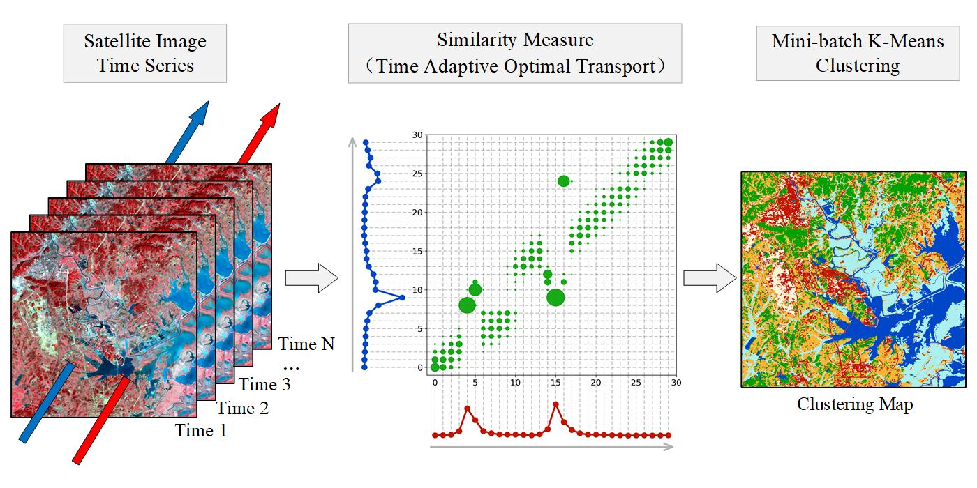
Satellite Image Time Series Clustering via Time Adaptive Optimal Transport

Abstract

Satellite Image Time Series (SITS) have become more accessible in recent years and SITS analysis has attracted increasing research interest. Given that labeled SITS training samples are time and effort consuming to acquire, clustering or unsupervised analysis methods need to be developed. Similarity measure is critical for clustering, however, currently established methods represented by Dynamic Time Warping (DTW) still exhibit several issues when coping with SITS, such as pathological alignment, sensitivity to spike noise, and limitation on capacity. In this paper, we introduce a new time series similarity measure method named time adaptive optimal transport (TAOT) to the application of SITS clustering. TAOT inherits several promising properties of optimal transport for the comparing of time series. Statistical and visual results on two real SITS datasets with two different settings demonstrate that TAOT can effectively alleviate the issues of DTW and further improve the clustering accuracy. Thus, TAOT can serve as a usable tool to explore the potential of precious SITS data.

1. Introduction

Recent years have witnessed a rapid growth of satellite imagery data sources [1,2], thanks to the launch of various new satellite sensors such as the GaoFen series [3], ZiYuan series [4], Sentinel-2 [5], etc. Historical data, for instance, MODIS imagery [6] and Landsat imagery [7], have also been accumulated over decades, making satellite image time series (SITS) data more accessible nowadays. Compared with a single-scene image, SITS records the evolution of land cover types over time and this kind of temporal information is sometimes critical to make land cover types more distinguishable [8,9,10]. In addition, image preprocessing methods required by SITS analytics, such as geometric correction [11,12] and cloud removal [13,14], become more mature than before. Due to the above reasons, SITS analytics has attracted much attention in recent years and many applications have been developed to explore the rich information contained in SITS, for example, classification [15,16], clustering [1,17], class noise reduction [18], trend detection [19], disturbance detection [20], etc.

Among different data mining tasks, clustering [21], or unsupervised classification, seems to gain more importance because the acquisition or update of labeled SITS training samples is difficult [1]. The difficulty comes from multiple aspects:

• All images contained in a SITS have to be considered simultaneously and a comprehensive judgement depending heavily on an expert’s knowledge has to be made.
• The land cover type of a SITS may change, especially when the time series is long and, thus, the class label itself is hard to decide in some cases.
• SITS data now have a higher temporal resolution so that labeled training samples can merely keep pace with the high data acquisition frequency.

Given the lack of labeled data, research on the clustering of SITS has gradually increased [10,17,22,23] with the focus on the similarity measure of time series [24,25]. Literature and applications show that Dynamic Time Warping (DTW) [26,27] based methods are probably the most relevant and successful time series similarity measures for SITS clustering tasks [1,28]. DTW was proposed in the field of speech recognition [26] and it soon became a significant tool to compare time series due to its capability to cope with time distortions. Time distortion is ubiquitous in time series and it is the main barrier for measuring similarities. DTW works by warping time series to find their optimal alignment that achieves the minimum global cost, and the cost is defined as the DTW distance. The paper by [1] analyzes the features and some unsolved issues of SITS, including irregular sampling, inconsistent temporal distortions, and cloud-contaminated pixels. Irregular sampling and inconsistent temporal distortions could be caused by satellite sensors or the irregular behaviors of observed objects, while cloud and cloud shadow cover is a common situation for optical satellite images. The paper then demonstrates that DTW could be a potential similarity measure to overcome these issues for the clustering of SITS. The essential reason is that DTW can warp and re-align those irregularities and distortions to recover a more “correct” similarity. In addition, the re-aligning mechanism enables DTW to compare time series with different lengths and thus make it possible to remove cloud-contaminated pixels first and then calculate similarities.

The versatility of DTW makes it a popular similarity measure framework for SITS under which various methods and applications emerge [23,29,30,31,32]. The paper by [33] uses DTW to define the difference measurement index for diagnosing vegetation recovery after a major earthquake. TWDTW [34], a time-weighted version of DTW, has been proposed for land cover mapping. The paper by [28] employs TWDTW to serve as the distance measure for cropland mapping with Sentinel-2 time series. TWDTW is also used for forest-type classification with both Landsat-8 and Sentinel-2 time series data by [35]. The CD-DTW [36] utilizes Canberra distance as the base cost of DTW and achieves accurate clustering of Landsat time series. The paper by [17] applies DTW to constrained clustering approaches and further improves the accuracy of SITS clustering. The paper by [37] introduces a weighted derivative modification of DTW for crops mapping with normalized difference vegetation index (NDVI) time series. Object-based DTW classifications are used for crop mapping by [16]. The paper by [38] proposes a phenology–time weighted version of DTW for winter wheat mapping over a large area based on the normalized difference phenology index (NDPI) curves derived from Sentinel-2 data.

However, despite many applications and modifications, DTW still exhibits several issues, especially when coping with SITS:

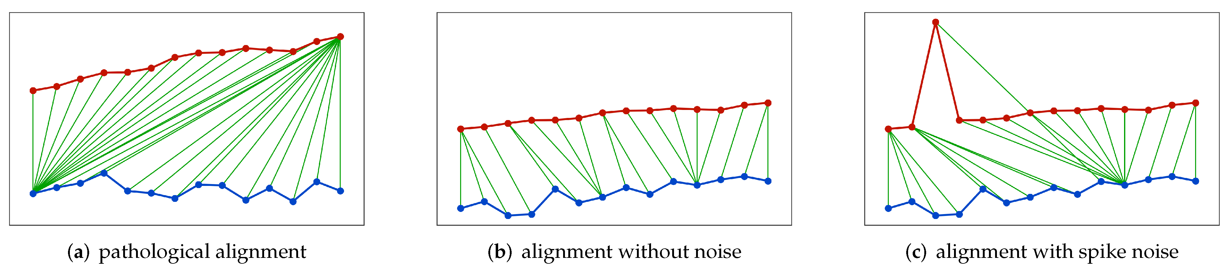
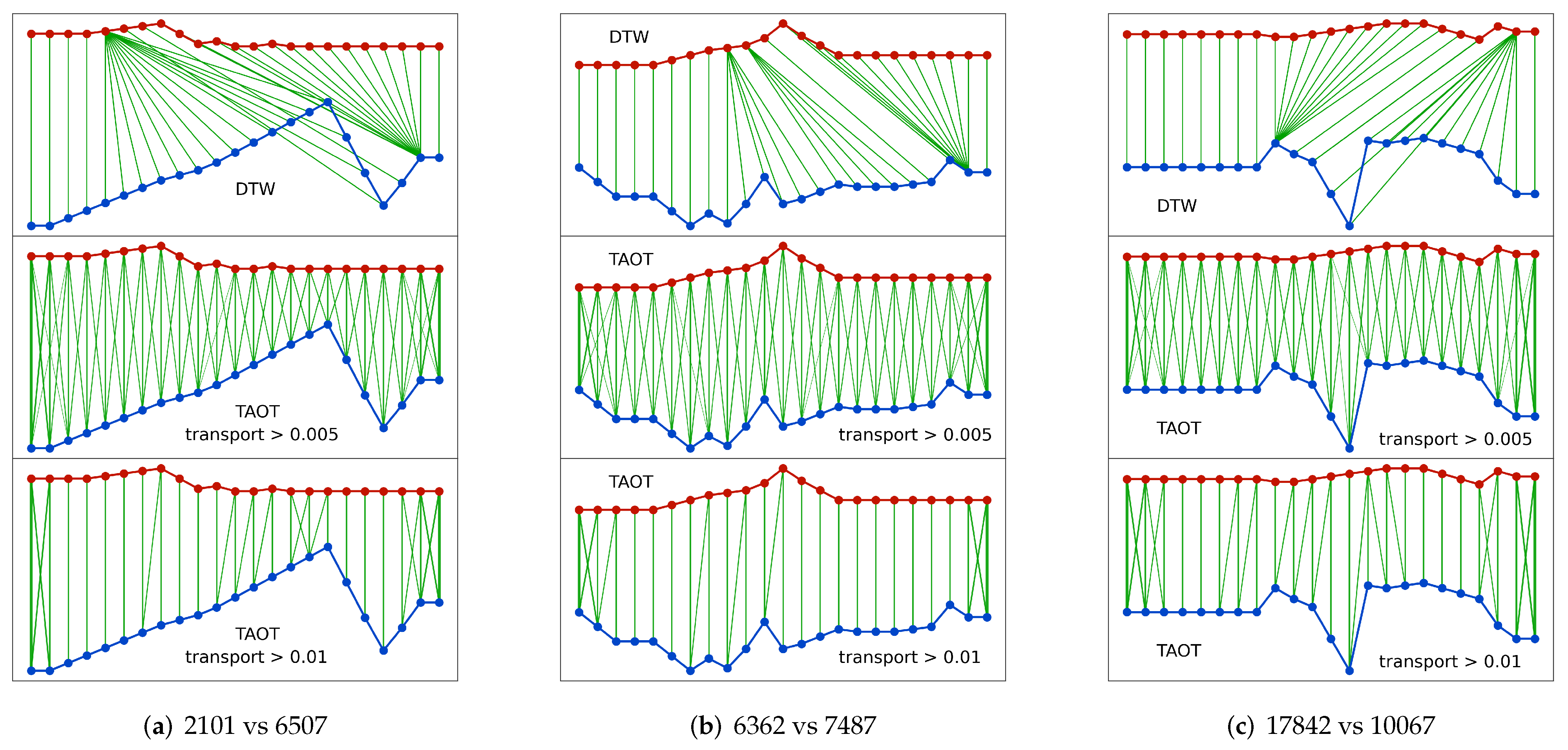
• Pathological alignment: A rational alignment between time series should be feature-to-feature and uniformly balanced, but DTW sometimes can lead to pathological alignment as shown by Figure 1a, where one point in a time series is mapped to nearly all points in the other time series, and this type of extreme alignment always ends with undesirable results.
• Spike noise: DTW is sensitive to spike noise as shown by Figure 1b,c, where a spike noise point easily disarranges the original alignment. Unluckily for SITS, spike noises such as cloud or cloud shadow pixels are ubiquitous and we cannot assume cloud-contaminated pixels will always be detected and removed completely.
• Limited capacity: The search space of optimal alignment is limited by DTW due to its rules of continuity, monotonicity, and boundary conditions. In theory, a fully-connected alignment can have a larger capacity and a higher flexibility for a more precise similarity.

These issues of DTW have long been noticed [39,40,41] but have not been effectively solved because they are directly related to the core definition of DTW [42]. Looking outside the context of DTW based methods, we find Optimal Transport (OT) [43,44,45] has theoretically promising properties to overcome the aforementioned issues of DTW. OT is a classic method to compare probability distributions or histograms [46,47,48] in that OT measures similarities by finding the minimum cost to transform one probability distribution to another. From the perspective of finding optimal cost OT is similar to DTW, but OT has a fuller search space than DTW because it is not constrained by temporal orders of data points or other rules of DTW. For a long time, the utility of OT had been limited by its high computational overhead [49] but recently a series of modifications have been proposed to significantly accelerate its computation. For instance, Sinkhorn distance [50] makes OT dozens of times faster while keeping approximately the same result.

Time series is different from probability distributions so that adaptation is required for OT to cope with time series data. In this paper, we introduce Time Adaptive Optimal Transport (TAOT) [42] as the similarity measure for the clustering of SITS. On the basis of Sinkhorn distance [50], TAOT enables OT to consider both observed values and their corresponding time coordinates simultaneously. In addition, TAOT assumes each data point in a time series to have the same probability and thus further simplifies the calculation. To demonstrate the performance of TAOT, we conduct SITS clustering experiments on two real SITS datasets in two different settings. The results are visually and statistically compared with multiple well-established similarity measures including Euclidean distance and DTW-based methods. To have an intuitive understanding of the mechanism of TAOT, we illustrate the alignments generated by TAOT and analyze their difference from DTW in detail. Other closely related topics such as parameter extracting and limitations of TAOT will also be discussed.

The rest of this article is structured as follows. Section 2 systematically describes time series similarity measures mainly from the perspective of alignment, and introduces OT and TAOT in detail. Section 3 presents the datasets, settings, and statistical and visual results of the SITS clustering experiments. Section 4 compares the alignments generated by TAOT and DTW, and discusses the limitations of TAOT. Finally, Section 5 concludes this paper.

2. Materials and Methods

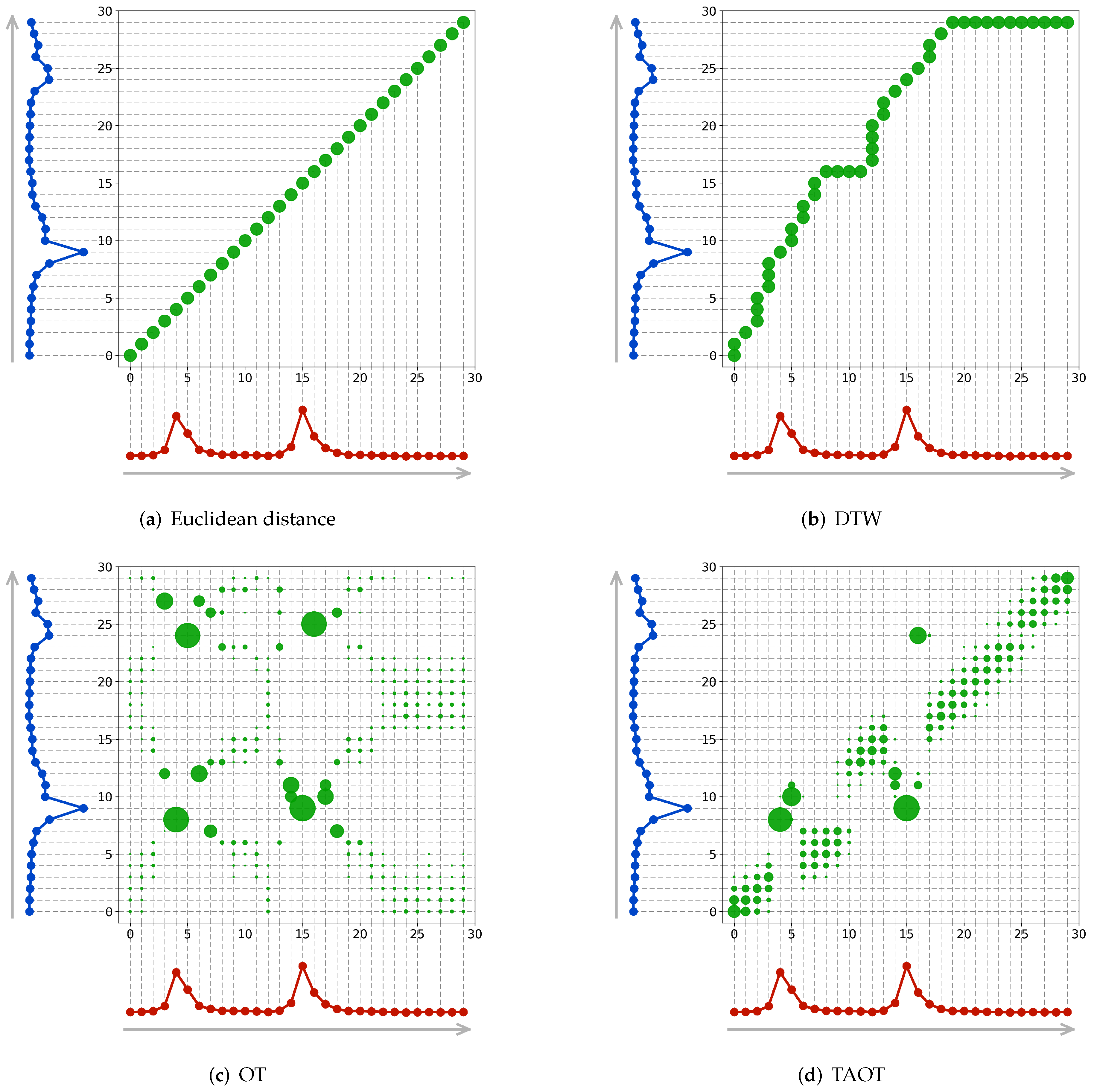
2.1. Alignment-Based Similarity Measures

A time series consists of a sequence of chronologically ordered data points. When two time series are compared, the real question can be described as how to align data points from different time series and how to measure the cost of each pair of points. From this perspective, many time series similarity measures can be classified as alignment-based methods, including the widely used Euclidean distance and Dynamic Time Warping (DTW) [26].

Euclidean distance is the most straightforward but still effective method. It enforces a strict one-to-one alignment in terms of time. Euclidean distance is usually viewed as the baseline method in the context of time series similarity measures.

Let $A=\{a_1,a_2,\dots ,a_i,\dots ,a_I\}$ and $B=\{b_1,b_2,\dots ,b_j,\dots ,b_J\}$ be two time series of length I and J, respectively. The lowercase $a_i$ and $b_j$ with subscript i and j denotes the i-th and j-th data points of A and B. Let $d(i,j)$ denote the cost between a pair of data points $a_i$ and $b_j$. Then the Euclidean distance (ED) between A and B can be defined as:

$$\begin{array}{cc}\hfill ED(A,B)& =\sum _{k=1}^{I}d(k,k)\hfill \\ \hfill I& =J\hfill \end{array}$$

(1)

where $d(i,j)={(a_i-b_j)}^2$. Note that the difference between $a_i$ and $b_j$ is squared because, in practice, squared Euclidean distance is more frequently used to save the square-root operation.

In contrast with Euclidean distance, DTW employs a more flexible one-to-many alignment that enables DTW to cope with time distortions effectively. There is only one case of one-to-one alignment, but many cases of one-to-many alignments. DTW attempts to find the optimal alignment with minimum accumulation cost. We use a warping path $W=w_1,w_2,\dots ,w_k,\dots ,w_K$ to represent the alignment between two time series A and B, where a time warp $w_k=(i,j)$ denotes a link between point $a_i$ and point $b_j$, and the total number of links or point pairs that compose the entire alignment is K. Pairwise cost between each pair of linked data points is added up to the final distance score. In this setting, DTW can be defined as:

$$\begin{array}{cc}\hfill DTW(A,B)& =\underset{W}{min}\sum _{k=1}^{K}d\left(w_k\right)\hfill \\ \hfill w_1& =(1,1)\hfill \\ \hfill w_K& =(I,J)\hfill \\ \hfill 0\le & i^{\prime }-i\le 1\hfill \\ \hfill 0\le & j^{\prime }-j\le 1\hfill \end{array}$$

(2)

where $w_k=(i,j)$, $w_{k+1}=(i^{\prime },j^{\prime })$, and $d\left(w_k\right)=d(i,j)={(a_i-b_j)}^2$.

The DTW problem defined by Equation (2) is essentially a dynamic programming problem and it can be solved by the following recursive formula:

$$DTW(A_i,B_j)=d(i,j)+min\left\{\begin{array}{c}DTW(A_i,B_{j-1})\hfill \\ DTW(A_{i-1},B_j)\hfill \\ DTW(A_{i-1},B_{j-1})\hfill \end{array}\right.$$

(3)

where $DTW(A_i,B_j)$ is the DTW distance between sub-sequences made up of the first i data points of A and the first j data points of B. $DTW(A_I,B_J)=DTW(A,B)$ is the final DTW distance between two entire time series.

Figure 2 illustrates the alignments generated by different methods. For each alignment, the x-axis and y-axis indicate the time coordinates of the two time series. An intersection point colored in green, for instance, $(i,j)$, indicates the i-th point in the first time series (colored in red) is aligned to the j-th point in the second time series (colored in blue), and all these green points together forms the warping path W. Figure 2a shows the alignment generated by Euclidean distance and we can observe that links happen only between points with the same time coordinate. Figure 2b shows the alignment generated by DTW where one point can link to multiple temporally adjacent points as long as the rules of DTW defined by Equation (2) are kept.

DTW is a well-established time series similarity measure framework under which many variants have been proposed. Variants of DTW can be classified into two major categories. The first category imposes constraints on DTW, for example, window constraint [51,52], weight constraint [34,53], slope constraint [54], warping path length constraint [41], etc. The second category replaces the feature DTW considers, for example, derivative DTW [39], piecewise DTW [55,56], shape context-based DTW [40], etc. In this paper, we employ the Sakoe–Chiba band [57,58] constrained DTW, piecewise DTW, and time-weighted DTW [34] to represent variants of DTW, and their performance will be compared with our proposed method. The Sakoe–Chiba band narrows the warping window of DTW using a constant radius r, which means for any $w_k=(i,j)$ in the warping path, $|i-j|\le r$. Piecewise DTW employs piecewise averages to replace the raw time series when calculating DTW. Time-weighted DTW adds a temporal cost to the cost between data points based on the date of each point when calculating DTW. Equation (4) formulates the cost between data points in time-weighted DTW.

$$\begin{array}{cc}\hfill d(i,j)& ={(a_i-b_j)}^2+\theta \ast \varphi (i,j)\hfill \\ \hfill \varphi (i,j)& =\frac{1}{1+e^{-\alpha \left(g\right(i,j)-\beta )}}\hfill \\ \hfill g(i,j)& =\left|doy\right(i)-doy(j\left)\right|\hfill \end{array}$$

(4)

where $d(i,j)$ denotes the cost between data points $a_i$ and $b_j$. $\theta$ is a weight coefficient for the temporal cost. $\varphi (i,j)$ is a logistic model with steepness $\alpha$ and midpoint $\beta$. $g(i,j)$ is the absolute difference between the day of year or Julian day of $a_i$ and $b_j$.

2.2. Time Adaptive Optimal Transport

Optimal Transport (OT) [43,59], also known as Earth Mover’s Distance [46,47] or Wasserstein Distance [60,61], has long been a theoretically ideal tool to compare probability distributions or histograms [48,62]. OT is modeled as the optimal solution to the supply–demand balanced transportation problem. Informally, suppose a series of mines providing iron ores and a series of factories consuming iron ores. The supply of each single mine or the demand of each single factory can be different but the total supply and the total demand are the same. Given the transport cost between each mine to each factory, OT can find the optimal transport allocation plan that leads to the minimum total cost while satisfying global supply-demand balance.

Given two probability distributions denoted as:

$$\begin{array}{cc}\hfill \left(A\right|P_A)& =\{\left(a_1\right|p_{a_1}),\left(a_2\right|p_{a_2}),\dots ,\left(a_i\right|p_{a_i}),\dots ,\left(a_d\right|p_{a_d})\}\hfill \\ \hfill \left(B\right|P_B)& =\{\left(b_1\right|p_{b_1}),\left(b_2\right|p_{b_2}),\dots ,\left(b_j\right|p_{b_j}),\dots ,\left(b_d\right|p_{b_d})\}\hfill \end{array}$$

(5)

where $a_i$ or $b_j$ is the i-th or j-th observed value in its respective distribution, and $p_{a_i}$ or $p_{b_j}$ is the corresponding probability of $a_i$ or $b_j$. Let $M=\left\{m_{ij}\right\}$ be the cost matrix between observed values of A and B, and typically $m_{ij}={(a_i-b_j)}^2$, then the OT distance can be defined as:

$$d_M(A,B):=\underset{P\in U(A,B)}{min}\sum _{i,j=1}^d{p}_{ij}{m}_{ij}$$

(6)

$$U(A,B):=\{P\in {\mathbb{R}}_{+}^{d\times d}|P{\mathbf{1}}_d=P_A,P^T{\mathbf{1}}_d=P_B\}$$

(7)

where ${\mathbf{1}}_d$ is a d-dimensional vector whose elements are all equal to 1, and $U(A,B)$ is the set containing all possible joint probabilities between A and B, whose row and column sums to $P_A$ and $P_B$, respectively.

The corresponding optimal transport plan $P^{★}$, is thus defined as:

$$P^{★}:=\underset{P\in U(A,B)}{argmin}\sum _{i,j=1}^d{p}_{ij}{m}_{ij}$$

(8)

From the definition of OT we can observe that OT has appealing mathematical properties to find the global optimal solution. However, the power comes with a large computational burden. OT has a worst case time complexity of $O\left(d^{3}logd\right)$ [49] that scales too fast even for a moderate-sized problem. After many attempts, a variant of OT named Sinkhorn distance [50] successfully makes OT dozens of times faster and reactivates the utility of OT. Sinkhorn distance adds an entropic regularization term to the classic OT equation to enforce a simple structure that has a fast solution. Sinkhorn distance is defined by the following equation:

$$d_M^{\lambda }(A,B):=\underset{P\in U(A,B)}{min}\left[\sum _{i,j=1}^d{p}_{ij}{m}_{ij}+\frac{1}{\lambda }\sum _{i,j=1}^d{p}_{ij}log{p}_{ij}\right]$$

(9)

where $\lambda$ is the regularization coefficient. A larger $\lambda$ leads to a weaker regularization and as $\lambda$ increases Sinkhorn distance converges to the raw OT distance. As the name implies, the regularized Equation (9) can be solved efficiently by Sinkhorn’s fixed point iteration.

From the perspective of finding minimum cost, OT is similar to DTW but OT considers a more general problem and, thus, OT has a larger capacity to find a more correct result. However, the downside is that OT is not originally designed for time series data and to some extent it neglects the nature of time series, namely the temporal order or the time coordinates of data points in a time series. To make OT capable of handling time series data, Time Adaptive Optimal Transport (TAOT) [42] has been proposed. TAOT simultaneously considers the observed values and their corresponding time coordinates when calculating the cost between each pair of data points. Concretely, the cost matrix in Equation (9) is now redefined as $M(i,j)={(a_i-b_j)}^2+w\ast {(t_i-t_j)}^2$, where $t_i$ and $t_j$ are z-scores of the time coordinates of $a_i$ and $b_j$, respectively, and w is a weight parameter for the tradeoff between the two parts. In addition, given the observation that data points in a time series are acquired at different times, TAOT assumes each data point is independent and thus has the same probability of $1/d$, where d is the total number of points in a time series as defined in Equation (5). In this setting, the Sinkhorn iteration can be further simplified and the detailed TAOT algorithm can be referred to in [42].

To have an intuitive impression of how OT and TAOT measure the similarity between time series, Figure 2c,d illustrates the alignments generated by OT and TAOT, respectively, where the radius of intersection points indicate the weights of connections. We can observe that both OT and TAOT lead to full connections among all points, although only some connections are strong while others are too weak to notice. Strong connections happen between corresponding peaks in the two time series and this characterizes an accurate alignment. Specifically, OT imposes no penalty on temporal distances and thus in Figure 2c connections (green circles) scatter around the whole area. In contrast, in Figure 2d most connections happen near the diagonal, the place where the temporal distance (difference between x and y coordinates) is small. This observation demonstrates that TAOT considers the temporal gap between points and penalizes connections with long temporal distances. In this setting, we can still find several strong connections (bigger green circles) a bit far from the diagonal, and this is because their numerical similarity dominates the temporal dissimilarity. In Figure 2c we can observe several strong connections (bigger green circles) in the upper left corner, however, due to their long temporal distances they are dismissed in Figure 2d.

A good alignment is expected to be feature-to-feature, where a local peak should be aligned to another temporally adjacent local peak in the other time series, and vice versa for local valleys. If a point is allowed to link with multiple points with different weights, then the weights of connections should consider the trade-off between numerical distance and temporal distance. In this standard, TAOT is better than DTW because TAOT generates more feature-to-feature connections and achieves the balance between numerical distance and temporal distance.

2.3. SITS Clustering with TAOT

A SITS clustering method usually requires two components: a similarity measure and a clustering algorithm. We introduce TAOT in this paper to serve as the similarity measure for SITS. As for the clustering algorithm, we choose mini-batch K-Means [63,64,65] for two main reasons. Firstly, mini-batch K-Means is a memory-saving algorithm. Compared with other categories of clustering algorithms such as density-based clustering, spectral clustering, or affinity propagation, mini-batch K-Means does not have to maintain a large distance matrix that scales quadratically with the number of samples. In contrast, mini-batch K-Means only has to maintain the distances to a limited number of cluster centers and the amount of memory scales linearly. Since satellite images always have millions of pixels, the memory-saving property becomes critical for the utility of a clustering algorithm. Secondly, given the same initial condition, the performance of mini-batch K-Means depends solely on the similarity measure and thus it ensures a fair comparison among different similarity measures.

The mini-batch K-Means [65] is a variant of K-Means that employs randomly sampled subsets instead of the entire sample set to update cluster centers during iterations. It drastically reduces the memory cost and the computation required to converge to the final solution, while still attempting to optimize the same global objective function as the raw K-Means. Generally, mini-batch K-Means produces results that are only slightly different than the raw K-Means. In this paper, we use the scikit-learn Python library to implement the mini-batch K-Means algorithm.

3. Results

To demonstrate the utility of TAOT for the clustering of SITS, in this section we evaluate the clustering accuracy of TAOT on two different datasets: the Reunion Island dataset and the Poyang Lake dataset. TAOT is compared with five well-established methods: Euclidean distance, DTW, Sakoe–Chiba band constrained DTW (SC-DTW), piecewise DTW (PDTW), and time-weighted DTW (TWDTW). To ensure a fair competition, we use the same initial cluster centers and the same random number generator such that the results depend only on the similarity measure.

Since the K-Means clustering algorithm is sensitive to initial cluster centers, and in order to demonstrate the utility of TAOT with different initial conditions, we conduct two groups of experiments for each dataset. The first experiment aims to estimate the best case capacity of these methods by using good initial cluster centers. Concretely, the first experiment employs the average time series of each class to be the initial cluster centers. The first experiment is technically semi-supervised because labeled samples are used for initialization. This scenario happens in real clustering tasks when we still have a few labeled samples. The second experiment uses 100 sets of random initial cluster centers and repeats the clustering procedure 100 times. The second experiment aims to evaluate the robustness under different conditions and is a traditional setting for clustering studies. Detailed results are shown, respectively, by the following Section 3.2 and Section 3.3.

3.1. Performance Metrics

The performance of each method is evaluated with four most widely used criteria: Adjusted Rand score, Cohen Kappa score, Overall Accuracy, and Weighted F1 score.

The Rand score [66,67] measures the similarity between two data clusterings from the perspective of sample pairs. For a total of n samples, the number of sample pairs is $n\ast (n-1)/2$. For two clusterings $C_1$ and $C_2$, let a be the number of pairs that are in the same clustering in $C1$ and in the same clustering in $C2$, and let b be the number of pairs that are in different clusterings in $C1$ and in different clusterings in $C2$. In this setting, $a+b$ expresses the number of agreements between $C1$ and $C2$. Then the Rand score is defined as the following Equation (10):

$$RS=\frac{a+b}{n\ast (n-1)/2}$$

(10)

The adjusted Rand score [68] is an adjusted-for-chance version of the Rand score that ensures a value close to 0 for two random clusterings and exactly $1.0$ for two identical clusterings. It is defined as the following Equation (11):

$$ARS=(RS-Expected(RS\left)\right)/\left(Max\right(RS)-Expected(RS\left)\right)$$

(11)

The Cohen Kappa score [69,70,71] is a statistic that measures the agreement between two classification results. It is defined as the following Equation (12):

$$\kappa =(p_o-p_e)/(1-p_e)$$

(12)

where $p_o$ is the observed agreement ratio and $p_e$ is the expected agreement ratio.

The overall accuracy is a straightforward performance metric, which is defined as the fraction of correct predictions. For a total of n samples, if $y_i$ is the real class label of the i-th sample and ${\widehat{y}}_i$ is the predicted class label, then the overall accuracy can be formulated as the following Equation (13):

$$accuracy=\frac{1}{n}\sum _{i=1}^{n}1\ast ({\widehat{y}}_i==y_i)$$

(13)

The F1 score [72,73] is the harmonic mean of precision and recall of a classifier. It is defined as the following Equation (14):

$$F_1=\frac{2}{precisio{n}^{-1}+recal{l}^{-1}}=2\ast \frac{precision\ast recall}{precision+recall}$$

(14)

where the precision is the number of true positive predictions divided by the number of all positive predictions, including those false positive predictions. In the context of classification, a true positive prediction means we predict a sample should belong to a certain class and it is true. A false positive prediction means we predict a sample should belong to a certain class but it is false. Precision reflects the ability of a classifier not to label as positive a sample that is negative. The recall is the number of true positive predictions divided by the number of all samples that should have been identified as positive. Recall reflects the ability of a classifier to find all the positive samples. In multi-class cases, the F1 score of each class is averaged and the weighted F1 score finds their average weighted by the number of samples of each class.

All of the four criteria described above range in $[0,1]$ and a higher value indicates a better result.

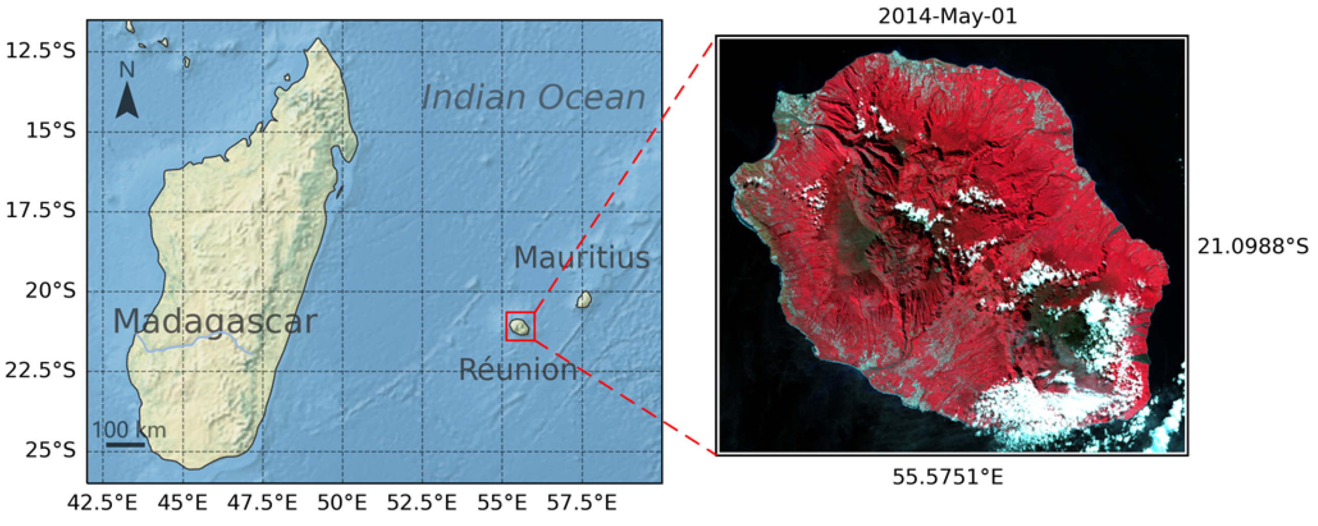
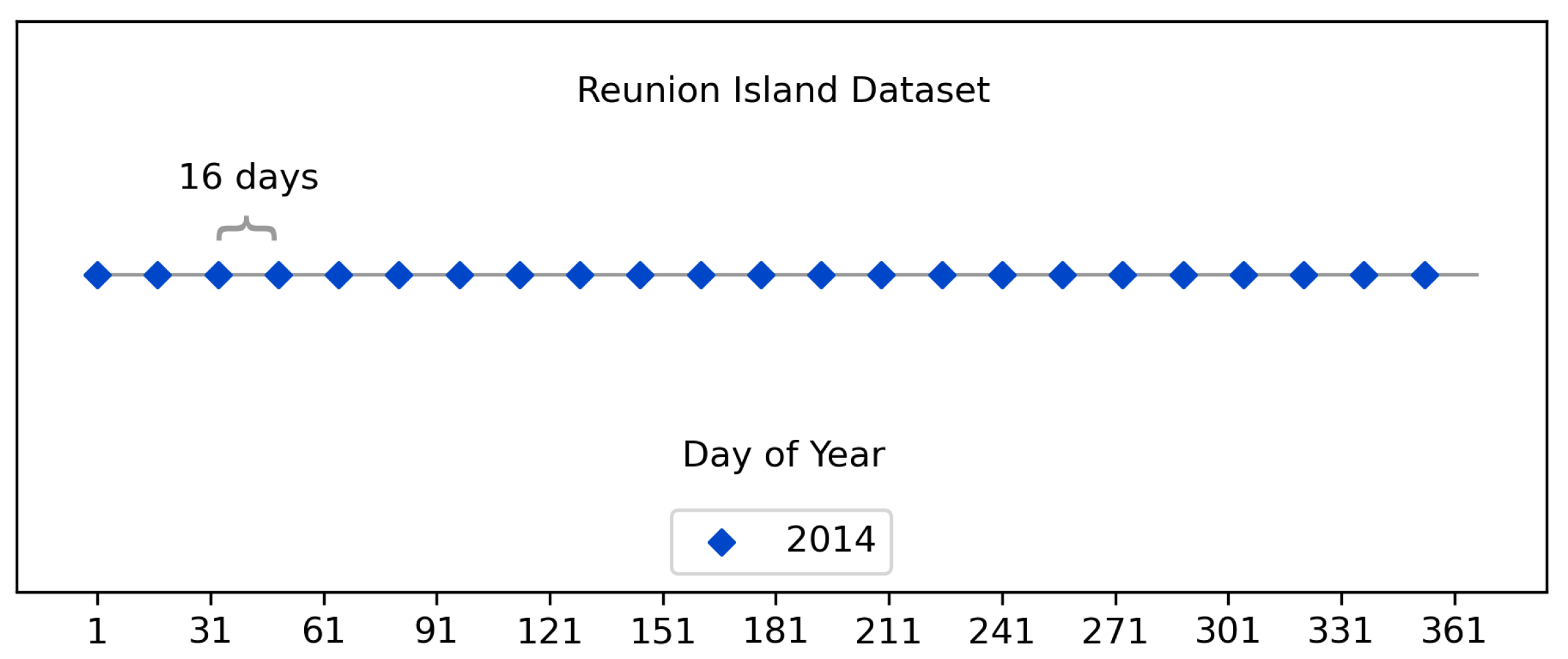
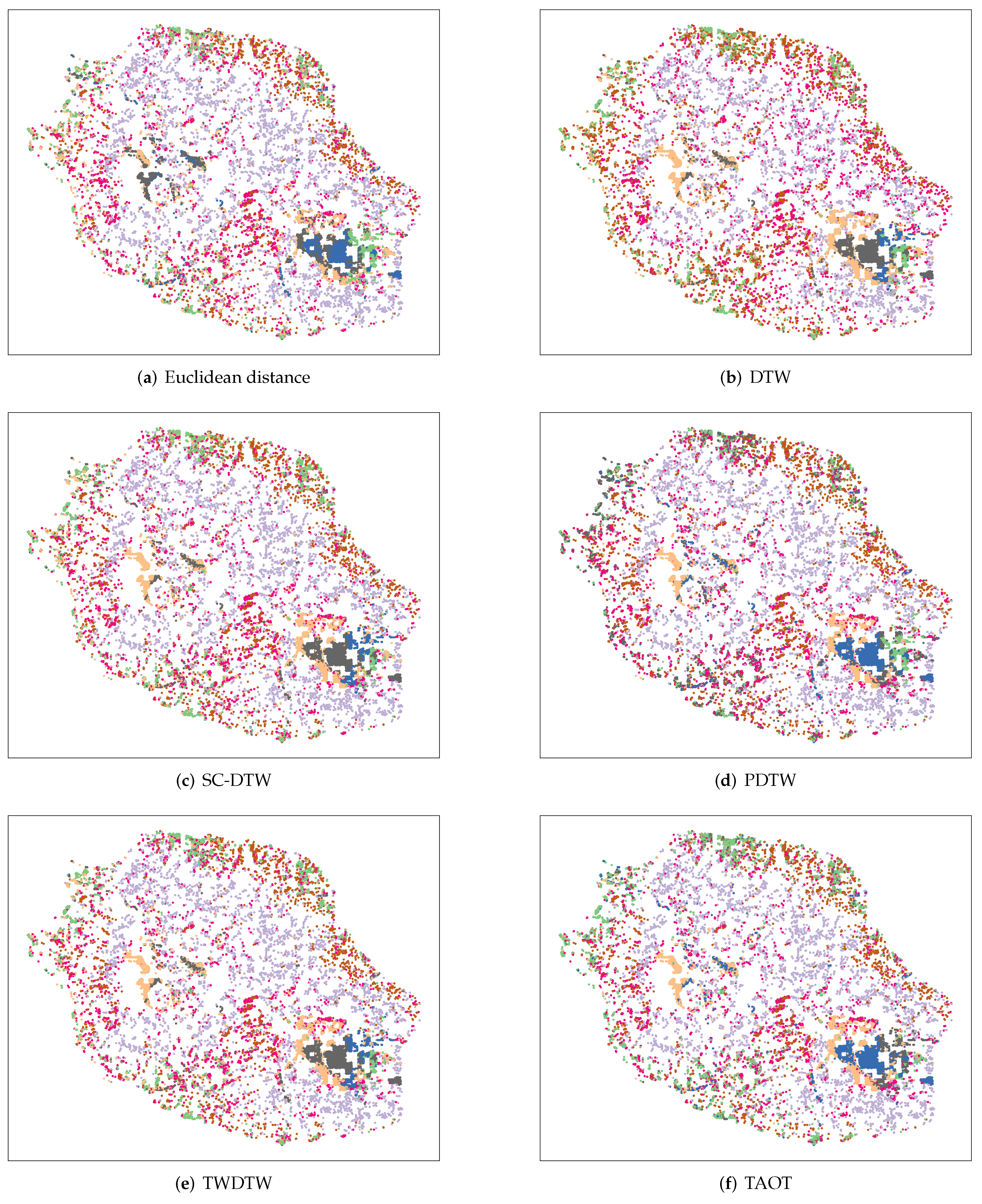
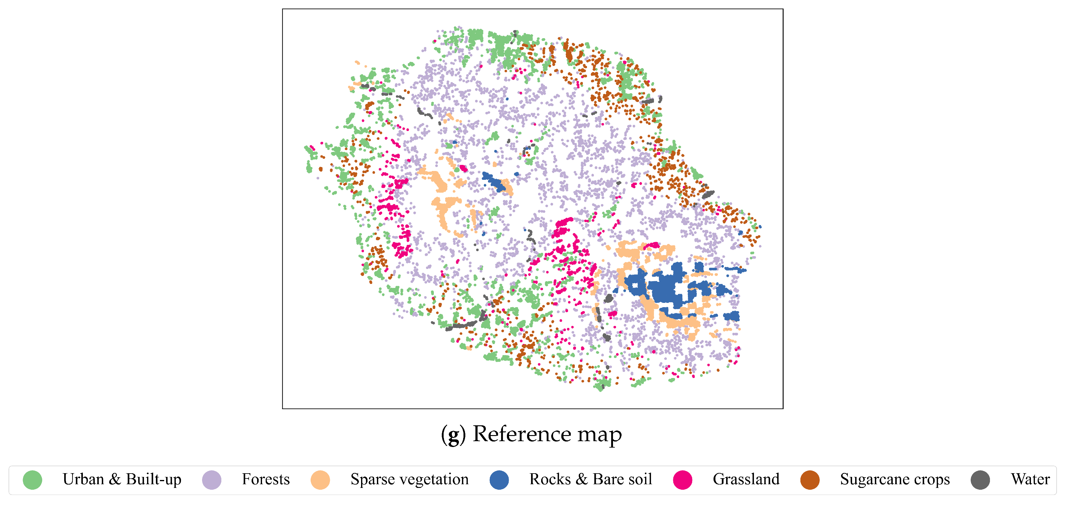
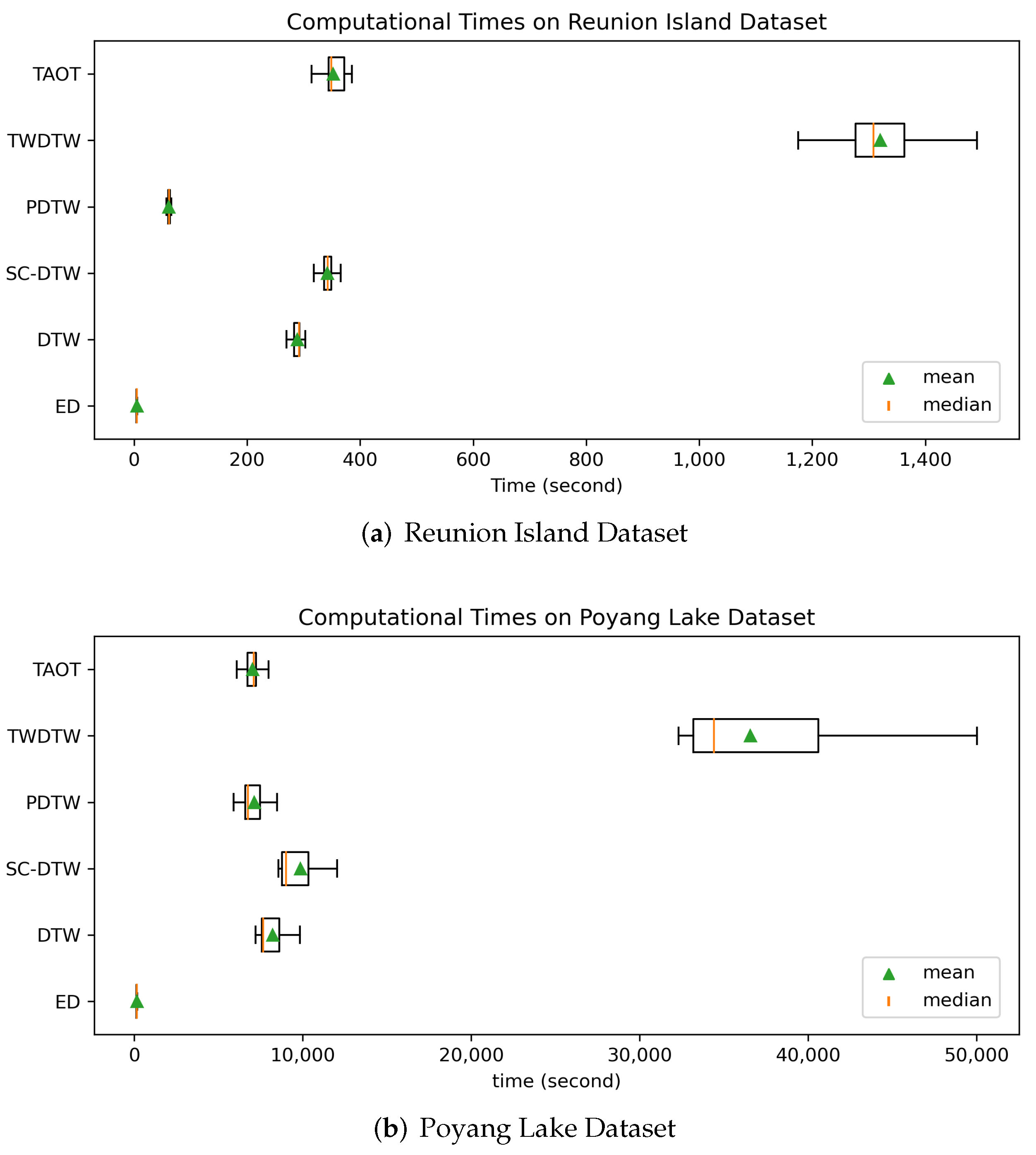
3.2. Reunion Island Dataset

The Reunion Island dataset was released by the Time Series Land Cover Classification Challenge (TiSeLaC) in the 2017 European Conference on Machine Learning & Principles and Practice of Knowledge Discovery in Databases (ECML/PKDD 2017). The study area covers the entire Reunion Island, a France overseas territory in the southwest Indian Ocean. Figure 3 illustrates the location and overview of the study area. The dataset is generated from an annual time series of 23 Landsat 8 images (30 m spatial resolution and 16 day temporal resolution) acquired in 2014. Figure 4 shows the temporal coverage of these images. Cloudy observations have been filled via pixel-wise multi-temporal linear interpolation on each multi-spectral band (OLI) independently. Each data point in a time series contains a total of 10 features, seven surface reflectance bands (Ultra Blue, Blue, Green, Red, NIR, SWIR1, and SWIR2) plus three complementary radiometric indices (NDVI, NDWI, and BI).

In the experiment we operate in an unsupervised manner and we conduct time series clustering on the testing set, which consists of 17,973 samples with ground truth class labels. To avoid the impact of imbalanced class distribution on the K-Means clustering algorithm and to focus on the comparison of similarity measures, two tiny classes whose sizes are not proportional to the other classes are respectively merged into their most similar classes. Concretely, the built-up class (647 samples) is merged into the urban class (4000 samples), and the other crops class (154 samples) is merged into the grassland class (1136 samples). The dataset is thus distributed over seven classes and

Table 1. Class distribution of the Reunion Island dataset.

Class ID	Class Name	Number of Samples	Percentage
1	Urban and built-up	4647	25.86%
2	Forests	4000	22.26%
3	Sparse vegetation	3398	18.91%
4	Rocks and bare soil	2588	14.40%
5	Grassland	1290	7.18%
6	Sugarcane crops	1531	8.52%
7	Water	519	2.89%
	Total	17,973	100.00%

reports the detailed class distribution.

Recall that two groups of experiments with different initial cluster centers are conducted.

Table 2. Comparison of clustering performance on Reunion Island dataset with averaged initial cluster centers. The best results are shown in bold.

Similarity Measure	ED	DTW	SC-DTW	PDTW	TWDTW	TAOT
Adjusted Rand Score	0.339	0.340	0.382	0.363	0.385	0.422
Cohen Kappa Score	0.433	0.409	0.458	0.458	0.453	0.554
Overall Accuracy	0.520	0.494	0.540	0.537	0.535	0.627
Weighted F1 Score	0.544	0.512	0.555	0.562	0.551	0.652

shows the clustering performance where the average time series of each class in the training set is used for initialization. The training set was released along with the testing set by TiSeLaC and it is used only in the first experiment for setting initial cluster centers. The performance is evaluated with four criteria described in the above Section 3.1. We can observe from Table 2 that TAOT consistently achieves the best results in terms of the four criteria, and TAOT wins by a relatively large margin of $3.7\%$, $9.6\%$, $8.7\%$, and $9.0\%$ compared to the second best result for each respective criterion.

Visually, Figure 5 shows the clustering maps generated by different similarity measures and the ground truth reference map. We can observe that the forest class (purple) is well recognized by all the five methods. However, Euclidean distance leads to significant confusion between sparse vegetation (orange) and water (gray). DTW, SC-DTW, and TWDTW lead to significant confusion between rocks and bare soil (blue) and water (gray). PDTW causes an obvious decrease of urban and built-up (green). Some of these issues also exist in the clustering map generated by TAOT, but they are alleviated in varying degrees.

Table 3. Comparison of clustering performance on Reunion Island dataset with random initial cluster centers. The best results are shown in bold.

Similarity Measure	ED	DTW	SC-DTW	PDTW	TWDTW	TAOT
Adjusted Rand Score	0.337 ± 0.043	0.335 ± 0.043	0.339 ± 0.043	0.332 ± 0.042	0.339 ± 0.042	0.352 ± 0.043
Cohen Kappa Score	0.306 ± 0.113	0.312 ± 0.118	0.311 ± 0.118	0.312 ± 0.113	0.309 ± 0.116	0.326 ± 0.117
Overall Accuracy	0.406 ± 0.101	0.410 ± 0.106	0.409 ± 0.106	0.411 ± 0.102	0.408 ± 0.105	0.424 ± 0.104
Weighted F1 Score	0.421 ± 0.108	0.428 ± 0.114	0.427 ± 0.114	0.428 ± 0.109	0.425 ± 0.112	0.446 ± 0.111

shows the clustering performance with 100 sets of random initial cluster centers on the Reunion Island dataset. The clustering is repeated 100 times and the average performance with standard deviation is reported. We can observe that in terms of all the four criteria, TAOT once again achieves the best results by margins of $1.3\%$, $1.4\%$, $1.3\%$, and $1.8\%$ compared to the second best result, respectively.

Figure 6 shows the distribution of each performance metric over the 100 repetitions performed on the Reunion Island dataset. We can observe that TAOT achieves the highest median, mean, maximum, and minimum in all the four box-plots.

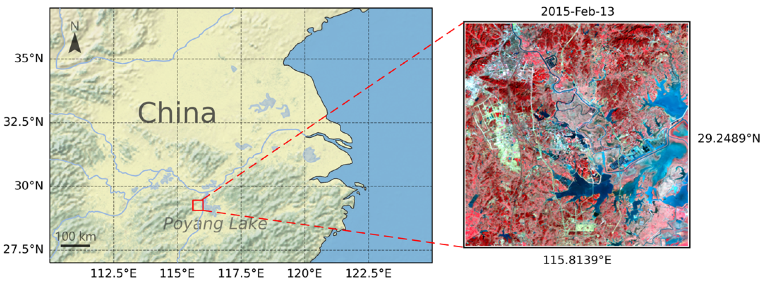
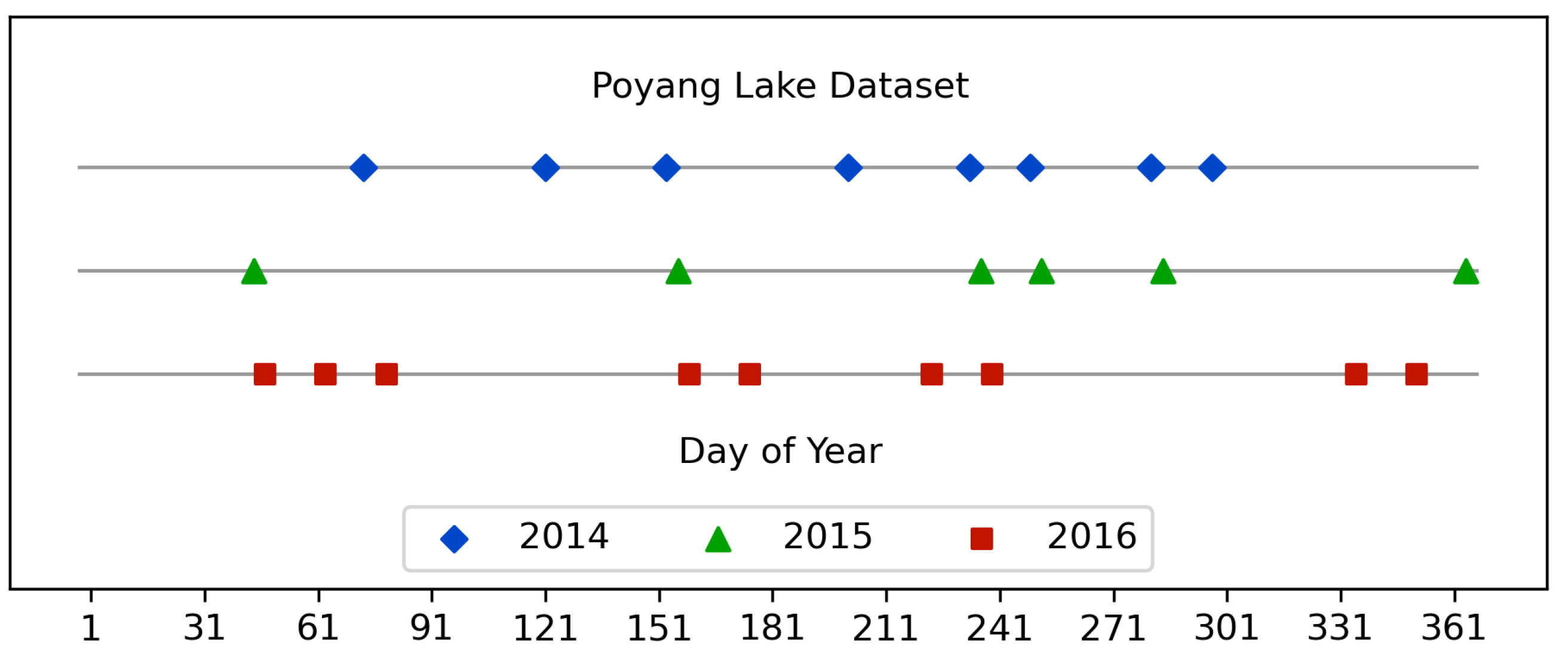
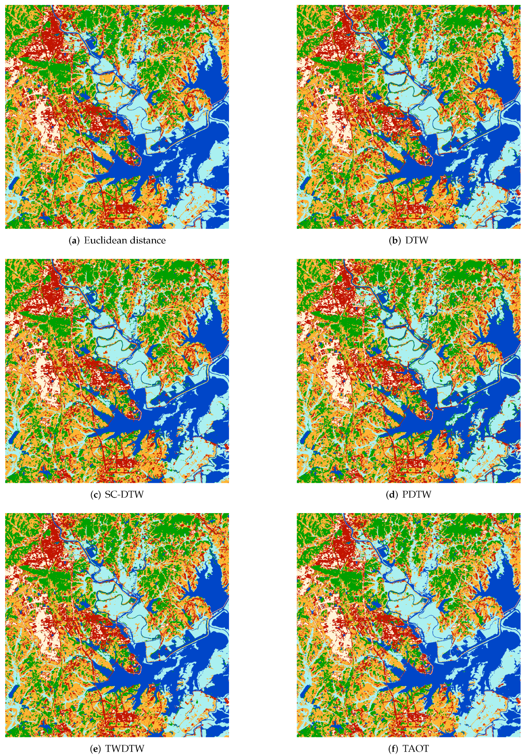
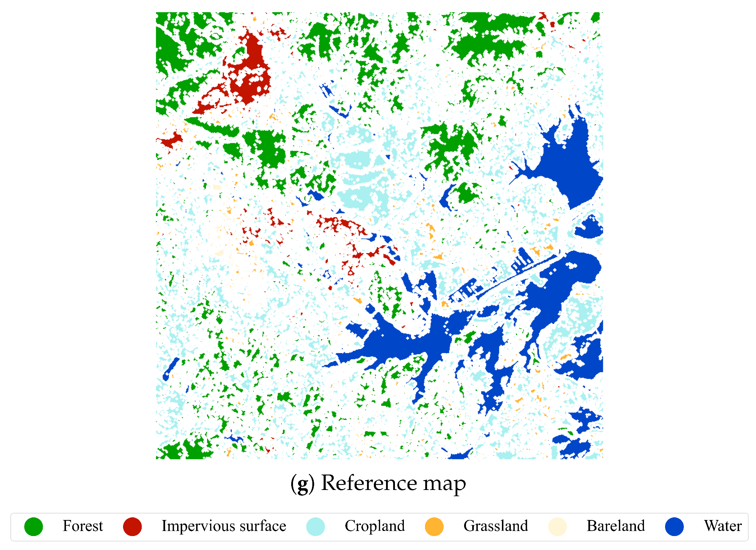
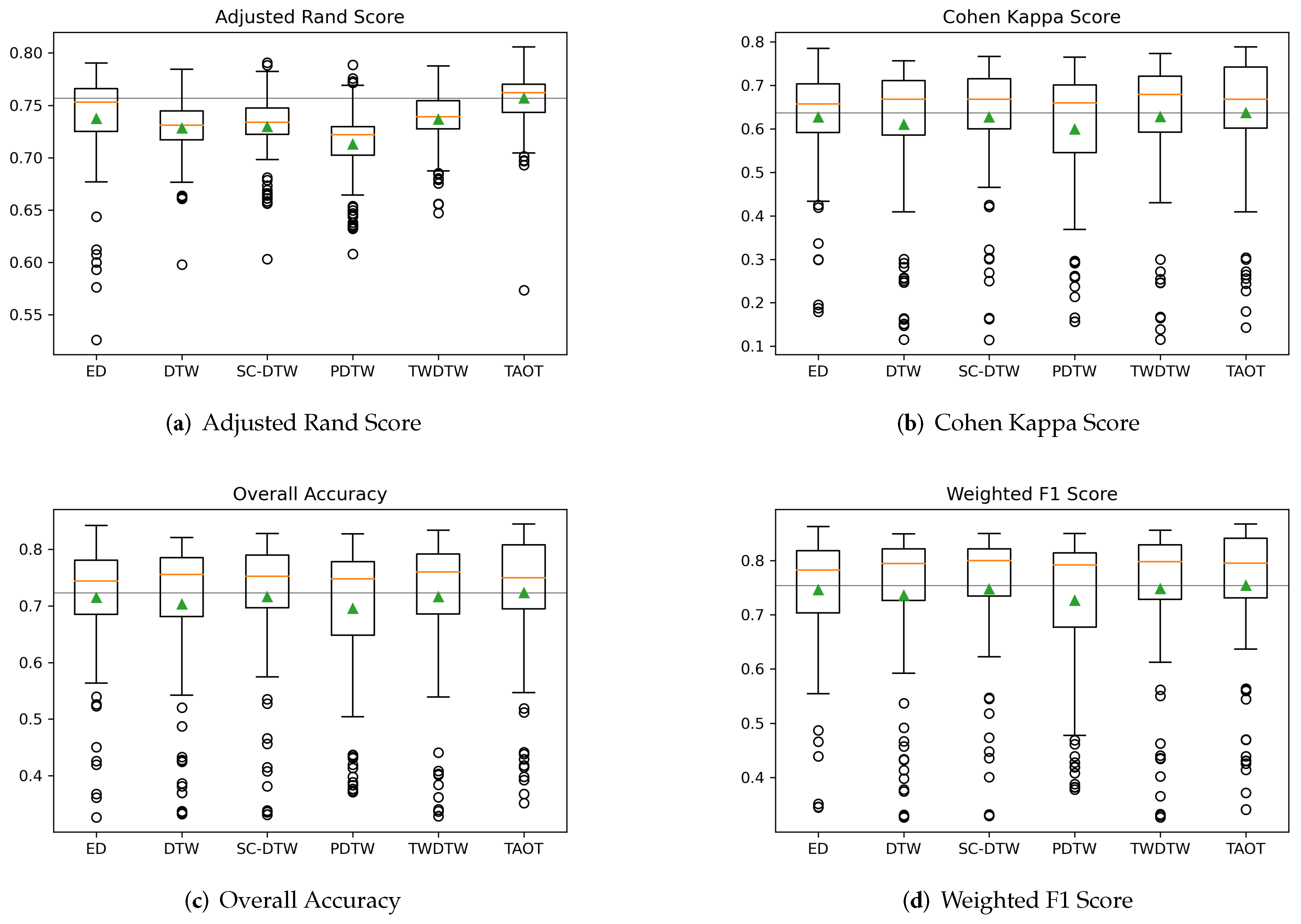
3.3. Poyang Lake Dataset

The Poyang Lake dataset consists of 23 cloud-free Landsat 8 land surface reflectance images acquired between 2014 and 2016. The study area is located in Poyang Lake, in the Jiangxi Province of China. Figure 7 illustrates the location and overview of the study area. We first mended cloud and cloud shadow pixels in each raw Landsat 8 image by the method proposed in [14] and then selected 23 clean images to construct the dataset. Figure 8 shows the temporal coverage of the selected images. We use the FROM-GLC 2015 (Finer Resolution Observation and Monitoring of Global Land Cover) classification product [74] (http://data.ess.tsinghua.edu.cn/ (accessed on 20 January 2021)) as ground truth reference. To further ensure the reliability of the reference set, we morphologically eroded the class labels with two iterations to keep only the central pixels of each land patch, because the central pixels are more likely to be correctly classified when generating the classification product. As the FROM-GLC 2015 product adopts different map projections, we reprojected Landsat images to the 0.00025 degrees per pixel geographic lat/lon projection used by FROM-GLC 2015. Each data point in a time series contains seven features, namely the seven surface reflectance bands (Ultra Blue, Blue, Green, Red, NIR, SWIR1, and SWIR2) of Landsat 8 imagery. The size of these images is $800\times 800$, where the coordinate of the upper-left corner of the first image (path: 121, row: 40, date: 2014-March-14) is $(1300,2050)$ in the entire scene.

The dataset contains six land cover classes: forest, impervious surface, cropland, grassland, bareland, and water.

Table 4. Class Ddistribution of the reference set of Poyang Lake dataset.

Class ID	Class Name	Number of Samples	Percentage
1	Cropland	47,181	27.68%
2	Forest	56,115	32.92%
3	Grassland	2937	1.72%
4	Water	54,262	31.83%
5	Impervious surface	9192	5.39%
6	Bareland	766	0.45%
	Total	170,453	100.00%

reports the detailed class distribution.

Table 5. Comparison of clustering performance on Poyang Lake dataset with averaged initial cluster centers. The best results are shown in bold.

Similarity Measure	ED	DTW	SC-DTW	PDTW	TWDTW	TAOT
Adjusted Rand Score	0.725	0.723	0.724	0.711	0.732	0.750
Cohen Kappa Score	0.714	0.723	0.728	0.716	0.731	0.749
Overall Accuracy	0.785	0.792	0.796	0.786	0.798	0.813
Weighted F1 Score	0.831	0.839	0.842	0.833	0.844	0.857

shows the clustering performance where average time series of each class in the reference set is used for initialization. The performance is also evaluated with the four criteria. We can observe that TAOT outperforms the other methods by margins of $1.8\%$, $1.8\%$, $1.5\%$, and $1.3\%$ compared to the second best result on each respective criterion. Visually, Figure 9 shows the clustering maps generated by different similarity measures and the morphologically eroded reference map. TAOT generates more precise contours for the majority of land cover patches.

Table 6. Comparison of clustering performance on Poyang Lake dataset with random initial cluster centers. The best results are shown in bold.

Similarity Measure	ED	DTW	SC-DTW	PDTW	TWDTW	TAOT
Adjusted Rand Score	0.737 ± 0.046	0.728 ± 0.032	0.730 ± 0.035	0.713 ± 0.039	0.737 ± 0.031	0.757 ± 0.030
Cohen Kappa Score	0.627 ± 0.124	0.610 ± 0.161	0.627 ± 0.138	0.599 ± 0.159	0.628 ± 0.154	0.637 ± 0.150
Overall Accuracy	0.715 ± 0.105	0.703 ± 0.129	0.716 ± 0.114	0.695 ± 0.127	0.716 ± 0.126	0.723 ± 0.123
Weighted F1 Score	0.746 ± 0.111	0.736 ± 0.138	0.747 ± 0.120	0.726 ± 0.133	0.748 ± 0.131	0.754 ± 0.128

shows the clustering performance with 100 sets of random initial cluster centers on the Poyang Lake dataset. The clustering is also repeated 100 times with the average performance and the standard deviation reported. We can observe that TAOT outperforms the other methods by margins of $2.0\%$, $0.9\%$, $0.7\%$, and $0.6\%$ compared to the second best result on each criterion.

Figure 10 shows the distribution of each performance metric over the 100 repetitions performed on the Poyang Lake dataset. For the adjusted Rand score, TAOT achieves the highest median, mean, maximum, and minimum by a relatively large margin. For the Cohen Kappa score, TAOT has the highest mean, maximum, and minimum, while TWDTW has a higher median (TAOT: 0.668, TWDTW: 0.679). For overall accuracy, TAOT has the highest mean and maximum. SC-DTW has a slightly larger minimum (TAOT: 0.695, SC-DTW: 0.696) and TWDTW has a larger median (TAOT: 0.750, TWDTW: 0.760). For the weighted F1 score, TAOT has the highest mean and maximum, while SC-DTW has the highest minimum (TAOT: 0.731, SC-DTW: 0.734) and median (TAOT: 0.795, SC-DTW: 0.800). The outliers illustrated by circles below the boxes are mainly caused by poor random initializations of cluster centers.

3.4. Extraction of Parameters

When parameters are involved in any similarity measure in the experiment, we search for the optimal values.

Table 7. Optimal parameters for each method on the two datasets.

Similarity Measure	ED	DTW	SC-DTW	PDTW	TWDTW	TAOT
Reunion Island Dataset	n/a	n/a	r = 3	n = 5	$\theta$ = 800,000, $\alpha$ = 0.1, $\beta$ = 100	$\lambda$ = 15, w = 400,000
Poyang Lake Dataset	n/a	n/a	r = 3	n = 21	$\theta$ = 600,000, $\alpha$ = 0.2, $\beta$ = 100	$\lambda$ = 12.5, w = 3,500,000

lists the optimal parameter values used in this paper. Euclidean distance and DTW are both parameter-free. SC-DTW has one parameter r, which is the radius of the Sakoe–Chiba band. PDTW also has one parameter n, which is the number of pieces. TWDTW has three parameters: the temporal weight coefficient $\theta$, the steepness $\alpha$, and the midpoint $\beta$ of the logistic weight model. TAOT involves two parameters: the regularization coefficient $\lambda$ and the temporal weight w. For SC-DTW and PDTW, as they are reference methods, we use the global optimal parameters found by linear search on the testing sets to show their best possible performance. For TWDTW, a linear search of $\theta$ with different combinations of $\alpha$ ($\alpha$ = 0.1 or 0.2) and $\beta$ ($\beta$ = 50, 100, 150, or 200) is conducted on the testing sets to find the optimal parameters. For TAOT, we find the optimal $\lambda$ and w by grid search on the training sets. If a full grid search is too time-consuming, we can search for w first with a coarse interval of $\lambda$, and then search for an optimal $\lambda$ with a dense interval given fixed w. Figure 11 illustrates the extraction process of $\lambda$ when the optimal w is decided.

4. Discussion

4.1. Alignments Generated by TAOT

A major motivation of using TAOT instead of DTW-based methods is to avoid the issues of pathological alignment and spike noise when coping with SITS data. Throughout this paper, similarity measure methods of time series are introduced from the perspective of alignments, and thus an intuitive way to see whether TAOT can solve these issues is to compare the alignments generated by different methods on real SITS datasets. Figure 12 illustrates three sets of alignments generated by DTW and TAOT on the TiSeLaC Reunion Island dataset. Recall that TAOT produces a fully-connected alignment represented by a transport matrix, but a large portion of the matrix cells have small values that are close to zero. To extract the essential part of the alignment and make it comparable with DTW, we filter the alignment of TAOT by weights of connections and only significant connections are kept. Two filter thresholds are adopted, where the smaller one (0.005) gives an overall impression of the alignment generated by TAOT, and the larger one (0.01) enables a comparison with DTW. In addition, we use the widths of lines to reflect the weights of connections.

In pathological alignments a point can be mapped onto an excessively large subsection of other points and distort the results. From all three sets of alignments shown in Figure 12 we find that DTW leads to pathological alignments locally in varying degrees, while TAOT leads to more balanced alignments. In Figure 12a,c we observe the appearance of spike noise and how it causes distortions to DTW. In contrast, TAOT is not obviously affected by the spike noise. These observations demonstrate our hypothesis that TAOT can alleviate the pathological alignment issue of DTW and it is not sensitive to spike noise. In addition, we observe that TAOT connections of points only happen in moderate temporal neighborhoods, which proves that TAOT achieves a trade-off between numerical and temporal similarities.

4.2. Capacity of TAOT

Another motivation of using TAOT is that TAOT derives a fully-connected alignment and thus theoretically has a larger capacity for a more precise result. The second row of Figure 12 shows that although weak connections are not drawn, each point still involves multiple connections with different weights. Rather than the many-to-many alignment generated by TAOT, DTW generates either one-to-many or many-to-one alignment. As a consequence, TAOT has a larger search space and more flexibility. Statistically, we have tested the capacity of TAOT in the previous experiments by giving each method an ideal initial condition and observing how well they could perform. On the Reunion Island dataset, TAOT outperforms the second best method by a large margin of $9.6\%$ in terms of the Cohen Kappa score, and on the Poyang Lake dataset the margin is $2.1\%$. This observation proves that TAOT can reach an obviously higher limit than the other well-established methods.

4.3. Limitations of TAOT

While TAOT has advantages on accuracy, its computational efficiency still has significant room for improvement. In theory, given two time series of length N, the time complexity of TAOT is approximately $O(N^{2}logN)$ [75], which is slower than DTW-based methods ($O\left(N^2\right)$) and Euclidean distance ($O\left(N\right)$). Note that the time complexity of naive optimal transport is $O(N^{3}logN)$ [49] and TAOT is already a faster variant of optimal transport.

In practice, Figure 13a,b shows the distribution of computational times for each method over the 100 repetitions performed on the two datasets, respectively. The times are measured on a configuration with 8 CPU cores of 2.5 GHz and 16-GB memory. We observe that Euclidean distance is the fastest due to its simplicity. Among DTW-based methods, PDTW is relatively rapid because it reduces the length of time series by piecewise averaging. TWDTW is the slowest on both the two datasets. TAOT runs moderately slower than DTW and SC-DTW on the Reunion Island dataset, which coincides with the theoretical analysis above. However, TAOT runs faster than DTW and SC-DTW on the Poyang Lake dataset. This might be because TAOT involves many matrix operations whose efficiency is better optimized when the size of matrices scale. Further acceleration of TAOT might be achieved through decomposing a multi-dimensional OT problem into one-dimensional ones and using one-dimensional results to compose the high-dimensional result [76].

Another issue of TAOT is that sometimes it will encounter the machine precision limit when $\lambda$ increases beyond a problem-dependent value ${\lambda }_{max}$, beyond which some elements of $e^{-\lambda M}$ are represented as zeroes. In this case we have to use a smaller $\lambda$ that may lead to a stricter regularization than desired.

5. Conclusions

In this paper, we have introduced time adaptive optimal transport (TAOT) as a similarity measure tool for satellite image time series (SITS), with the aim of avoiding the issues of DTW-based methods, namely the pathological alignment, sensitivity to spike noise, and limitation on capacity. TAOT is derived from the classic optimal transport framework which has long been a powerful tool to compare probability distributions or histograms. In addition, TAOT further considers temporal similarities to make it suitable for SITS data. In order to demonstrate the properties of TAOT, we have presented SITS clustering experiments on two real SITS datasets in two different settings. TAOT consistently outperformed the other methods in terms of four well-established accuracy criteria. To gain a deeper understanding of TAOT, we have illustrated the alignments generated by TAOT and compared them with DTW. TAOT is able to generate a more balanced fully-connected alignment to precisely capture the similarity between time series, and thus TAOT can serve as a usable tool for the analysis of complex SITS data.

References

1. Petitjean, F.; Inglada, J.; Gançarski, P. Satellite image time series analysis under time warping. IEEE Trans. Geosci. Remote Sens. 2012, 50, 3081–3095. [Google Scholar] [CrossRef]
2. Pelletier, C.; Webb, G.I.; Petitjean, F. Temporal convolutional neural network for the classification of satellite image time series. Remote Sens. 2019, 11, 523. [Google Scholar] [CrossRef] [Green Version]
3. Li, Z.; Shen, H.; Li, H.; Xia, G.; Gamba, P.; Zhang, L. Multi-feature combined cloud and cloud shadow detection in GaoFen-1 wide field of view imagery. Remote Sens. Environ. 2017, 191, 342–358. [Google Scholar] [CrossRef] [Green Version]
4. Tang, X.; Zhang, G.; Zhu, X.; Pan, H.; Jiang, Y.; Zhou, P.; Wang, X. Triple linear-array image geometry model of ZiYuan-3 surveying satellite and its validation. Int. J. Image Data Fusion 2013, 4, 33–51. [Google Scholar] [CrossRef]
5. Drusch, M.; Del Bello, U.; Carlier, S.; Colin, O.; Fernandez, V.; Gascon, F.; Hoersch, B.; Isola, C.; Laberinti, P.; Martimort, P.; et al. Sentinel-2: ESA’s optical high-resolution mission for GMES operational services. Remote Sens. Environ. 2012, 120, 25–36. [Google Scholar] [CrossRef]
6. Justice, C.; Townshend, J.; Vermote, E.; Masuoka, E.; Wolfe, R.; Saleous, N.; Roy, D.; Morisette, J. An overview of MODIS Land data processing and product status. Remote Sens. Environ. 2002, 83, 3–15. [Google Scholar] [CrossRef]
7. Williams, D.L.; Goward, S.; Arvidson, T. Landsat. Photogramm. Eng. Remote Sens. 2006, 72, 1171–1178. [Google Scholar] [CrossRef]
8. Pelletier, C.; Valero, S.; Inglada, J.; Champion, N.; Dedieu, G. Assessing the robustness of Random Forests to map land cover with high resolution satellite image time series over large areas. Remote Sens. Environ. 2016, 187, 156–168. [Google Scholar] [CrossRef]
9. Inglada, J.; Vincent, A.; Arias, M.; Tardy, B.; Morin, D.; Rodes, I. Operational High Resolution Land Cover Map Production at the Country Scale Using Satellite Image Time Series. Remote Sens. 2017, 9, 95. [Google Scholar] [CrossRef] [Green Version]
10. Khiali, L.; Ndiath, M.; Alleaume, S.; Ienco, D.; Ose, K.; Teisseire, M. Detection of spatio-temporal evolutions on multi-annual satellite image time series: A clustering based approach. Int. J. Appl. Earth Obs. Geoinf. 2019, 74, 103–119. [Google Scholar] [CrossRef]
11. Gonçalves, H.; Gonçalves, J.A.; Corte-Real, L. Measures for an objective evaluation of the geometric correction process quality. IEEE Geosci. Remote Sens. Lett. 2009, 6, 292–296. [Google Scholar] [CrossRef]
12. Habib, A.; Han, Y.; Xiong, W.; He, F.; Zhang, Z.; Crawford, M. Automated ortho-rectification of UAV-based hyperspectral data over an agricultural field using frame RGB imagery. Remote Sens. 2016, 8, 796. [Google Scholar] [CrossRef] [Green Version]
13. Lin, C.H.; Tsai, P.H.; Lai, K.H.; Chen, J.Y. Cloud removal from multitemporal satellite images using information cloning. IEEE Trans. Geosci. Remote Sens. 2012, 51, 232–241. [Google Scholar] [CrossRef]
14. Hu, C.; Huo, L.Z.; Zhang, Z.; Tang, P. Multi-temporal landsat data automatic cloud removal using poisson blending. IEEE Access 2020, 8, 46151–46161. [Google Scholar] [CrossRef]
15. Pelletier, C.; Valero, S.; Inglada, J.; Champion, N.; Marais Sicre, C.; Dedieu, G. Effect of training class label noise on classification performances for land cover mapping with satellite image time series. Remote Sens. 2017, 9, 173. [Google Scholar] [CrossRef] [Green Version]
16. Csillik, O.; Belgiu, M.; Asner, G.P.; Kelly, M. Object-based time-constrained dynamic time warping classification of crops using Sentinel-2. Remote Sens. 2019, 11, 1257. [Google Scholar] [CrossRef] [Green Version]
17. Lampert, T.; Lafabregue, B.; Gançarski, P. Constrained distance based k-means clustering for satellite image time-series. In Proceedings of the IGARSS 2019—2019 IEEE International Geoscience and Remote Sensing Symposium, Yokohama, Japan, 28 July–2 August 2019; pp. 2419–2422. [Google Scholar]
18. Santos, L.A.; Ferreira, K.R.; Camara, G.; Picoli, M.C.; Simoes, R.E. Quality control and class noise reduction of satellite image time series. ISPRS J. Photogramm. Remote Sens. 2021, 177, 75–88. [Google Scholar] [CrossRef]
19. Verbesselt, J.; Hyndman, R.; Newnham, G.; Culvenor, D. Detecting trend and seasonal changes in satellite image time series. Remote Sens. Environ. 2010, 114, 106–115. [Google Scholar] [CrossRef]
20. Kong, Y.L.; Huang, Q.; Wang, C.; Chen, J.; Chen, J.; He, D. Long short-term memory neural networks for online disturbance detection in satellite image time series. Remote Sens. 2018, 10, 452. [Google Scholar] [CrossRef] [Green Version]
21. Liao, T.W. Clustering of time series data—A survey. Pattern Recognit. 2005, 38, 1857–1874. [Google Scholar] [CrossRef]
22. Gonçalves, R.; Zullo, J.; Amaral, B.F.D.; Coltri, P.P.; Sousa, E.P.M.D.; Romani, L.A.S. Land use temporal analysis through clustering techniques on satellite image time series. In Proceedings of the 2014 IEEE Geoscience and Remote Sensing Symposium, Quebec City, QC, Canada, 13–18 July 2014; pp. 2173–2176. [Google Scholar]
23. Zhang, Y.; Zhao, H. Land–use and land-cover change detection using dynamic time warping–based time series clustering method. Can. J. Remote Sens. 2020, 46, 67–83. [Google Scholar] [CrossRef]
24. Fu, T.c. A review on time series data mining. Eng. Appl. Artif. Intell. 2011, 24, 164–181. [Google Scholar] [CrossRef]
25. Mori, U.; Mendiburu, A.; Lozano, J.A. Similarity measure selection for clustering time series databases. IEEE Trans. Knowl. Data Eng. 2015, 28, 181–195. [Google Scholar] [CrossRef]
26. Sakoe, H.; Chiba, S. Dynamic programming algorithm optimization for spoken word recognition. IEEE Trans. Acoust. Speech Signal Process. 1978, 26, 43–49. [Google Scholar] [CrossRef] [Green Version]
27. Müller, M. Dynamic time warping. In Information Retrieval for Music and Motion; Springer: Berlin/Heidelberg, Germany, 2007; pp. 69–84. [Google Scholar]
28. Belgiu, M.; Csillik, O. Sentinel-2 cropland mapping using pixel-based and object-based time-weighted dynamic time warping analysis. Remote Sens. Environ. 2018, 204, 509–523. [Google Scholar] [CrossRef]
29. Weber, J.; Petitjean, F.; Gançarski, P. Towards efficient satellite image time series analysis: Combination of dynamic time warping and quasi-flat zones. In Proceedings of the 2012 IEEE International Geoscience and Remote Sensing Symposium, Munich, Germany, 22–27 July 2012; pp. 4387–4390. [Google Scholar]
30. Mondal, S.; Jeganathan, C. Mountain agriculture extraction from time-series MODIS NDVI using dynamic time warping technique. Int. J. Remote Sens. 2018, 39, 3679–3704. [Google Scholar] [CrossRef]
31. Li, M.; Bijker, W. Vegetable classification in Indonesia using Dynamic Time Warping of Sentinel-1A dual polarization SAR time series. Int. J. Appl. Earth Obs. Geoinf. 2019, 78, 268–280. [Google Scholar] [CrossRef]
32. Moola, W.S.; Bijker, W.; Belgiu, M.; Li, M. Vegetable mapping using fuzzy classification of Dynamic Time Warping distances from time series of Sentinel-1A images. Int. J. Appl. Earth Obs. Geoinf. 2021, 102, 102405. [Google Scholar] [CrossRef]
33. Zhang, X.; Wang, M.; Liu, K.; Xie, J.; Xu, H. Using NDVI time series to diagnose vegetation recovery after major earthquake based on dynamic time warping and lower bound distance. Ecol. Indic. 2018, 94, 52–61. [Google Scholar] [CrossRef]
34. Maus, V.; Câmara, G.; Cartaxo, R.; Sanchez, A.; Ramos, F.M.; De Queiroz, G.R. A time-weighted dynamic time warping method for land-use and land-cover mapping. IEEE J. Sel. Top. Appl. Earth Obs. Remote Sens. 2016, 9, 3729–3739. [Google Scholar] [CrossRef]
35. Cheng, K.; Wang, J. Forest-Type Classification Using Time-Weighted Dynamic Time Warping Analysis in Mountain Areas: A Case Study in Southern China. Forests 2019, 10, 1040. [Google Scholar] [CrossRef] [Green Version]
36. Zhao, Y.; Lin, L.; Lu, W.; Meng, Y. Landsat time series clustering under modified Dynamic Time Warping. In Proceedings of the 2016 4th International Workshop on Earth Observation and Remote Sensing Applications (EORSA), Guangzhou, China, 4–6 July 2016; pp. 62–66. [Google Scholar]
37. Belgiu, M.; Zhou, Y.; Marshall, M.; Stein, A. Dynamic time warping for crops mapping. Int. Arch. Photogramm. Remote Sens. Spat. Inf. Sci. 2020, 43, 947–951. [Google Scholar] [CrossRef]
38. Dong, Q.; Chen, X.; Chen, J.; Zhang, C.; Liu, L.; Cao, X.; Zang, Y.; Zhu, X.; Cui, X. Mapping winter wheat in North China using Sentinel 2A/B data: A method based on phenology-time weighted dynamic time warping. Remote Sens. 2020, 12, 1274. [Google Scholar] [CrossRef] [Green Version]
39. Keogh, E.J.; Pazzani, M.J. Derivative dynamic time warping. In Proceedings of the 2001 SIAM International Conference on Data Mining, Chicago, IL, USA, 5 April 2021; SIAM: Philadelphia, PA, USA, 2001; pp. 1–11. [Google Scholar]
40. Zhang, Z.; Tang, P.; Duan, R. Dynamic time warping under pointwise shape context. Inf. Sci. 2015, 315, 88–101. [Google Scholar] [CrossRef]
41. Zhang, Z.; Tavenard, R.; Bailly, A.; Tang, X.; Tang, P.; Corpetti, T. Dynamic Time Warping under limited warping path length. Inf. Sci. 2017, 393, 91–107. [Google Scholar] [CrossRef] [Green Version]
42. Zhang, Z.; Tang, P.; Corpetti, T. Time Adaptive Optimal Transport: A Framework of Time Series Similarity Measure. IEEE Access 2020, 8, 149764–149774. [Google Scholar] [CrossRef]
43. Villani, C. Optimal Transport: Old and New; Springer Science & Business Media: Berlin, Germany, 2008; Volume 338. [Google Scholar]
44. Peyré, G.; Cuturi, M. Computational optimal transport: With applications to data science. Found. Trends Mach. Learn. 2019, 11, 355–607. [Google Scholar] [CrossRef]
45. Santambrogio, F. Optimal transport for applied mathematicians. Birkäuser N. Y. 2015, 55, 94. [Google Scholar]
46. Rubner, Y.; Tomasi, C.; Guibas, L.J. The earth mover’s distance as a metric for image retrieval. Int. J. Comput. Vis. 2000, 40, 99–121. [Google Scholar] [CrossRef]
47. Ling, H.; Okada, K. An efficient earth mover’s distance algorithm for robust histogram comparison. IEEE Trans. Pattern Anal. Mach. Intell. 2007, 29, 840–853. [Google Scholar] [CrossRef] [PubMed]
48. Courty, N.; Flamary, R.; Tuia, D.; Rakotomamonjy, A. Optimal transport for domain adaptation. IEEE Trans. Pattern Anal. Mach. Intell. 2017, 39, 1853–1865. [Google Scholar] [CrossRef]
49. Pele, O.; Werman, M. Fast and robust earth mover’s distances. In Proceedings of the 2009 IEEE 12th International Conference on Computer Vision, Kyoto, Japan, 29 September–2 October 2009; pp. 460–467. [Google Scholar]
50. Cuturi, M. Sinkhorn distances: Lightspeed computation of optimal transport. Adv. Neural Inf. Process. Syst. 2013, 26, 2292–2300. [Google Scholar]
51. Berndt, D.J.; Clifford, J. Using dynamic time warping to find patterns in time series. In Proceedings of the KDD Workshop, Seattle, WA, USA, 31 July 1994; pp. 359–370. [Google Scholar]
52. Ratanamahatana, C.A.; Keogh, E. Making time-series classification more accurate using learned constraints. In Proceedings of the 2004 SIAM International Conference on Data Mining, Lake Buena Vista, FL, USA, 22 April 2014; SIAM: Philadelphia, PA, USA, 2004; pp. 11–22. [Google Scholar]
53. Jeong, Y.S.; Jeong, M.K.; Omitaomu, O.A. Weighted dynamic time warping for time series classification. Pattern Recognit. 2011, 44, 2231–2240. [Google Scholar] [CrossRef]
54. Myers, C.; Rabiner, L.; Rosenberg, A. Performance tradeoffs in dynamic time warping algorithms for isolated word recognition. IEEE Trans. Acoust. Speech Signal Process. 1980, 28, 623–635. [Google Scholar] [CrossRef]
55. Keogh, E.J.; Pazzani, M.J. Scaling up dynamic time warping for datamining applications. In Proceedings of the Sixth ACM SIGKDD International Conference on Knowledge Discovery and Data Mining, Boston, MA, USA, 20–23 August 2000; pp. 285–289. [Google Scholar]
56. Cai, Q.; Chen, L.; Sun, J. Piecewise statistic approximation based similarity measure for time series. Knowl.-Based Syst. 2015, 85, 181–195. [Google Scholar] [CrossRef]
57. Geler, Z.; Kurbalija, V.; Radovanović, M.; Ivanović, M. Impact of the Sakoe-Chiba band on the DTW time series distance measure for kNN classification. In International Conference on Knowledge Science, Engineering and Management; Springer: Cham, Switzerland, 2014; pp. 105–114. [Google Scholar]
58. Górecki, T.; Łuczak, M. The influence of the Sakoe–Chiba band size on time series classification. J. Intell. Fuzzy Syst. 2019, 36, 527–539. [Google Scholar] [CrossRef]
59. Rubner, Y.; Tomasi, C.; Guibas, L.J. A metric for distributions with applications to image databases. In Proceedings of the Sixth International Conference on Computer Vision, Bombay, India, 7 January 1998; pp. 59–66. [Google Scholar]
60. Piccoli, B.; Rossi, F. Generalized Wasserstein distance and its application to transport equations with source. Arch. Ration. Mech. Anal. 2014, 211, 335–358. [Google Scholar] [CrossRef] [Green Version]
61. Robin, Y.; Yiou, P.; Naveau, P. Detecting changes in forced climate attractors with Wasserstein distance. Nonlinear Process. Geophys. 2017, 24, 393. [Google Scholar] [CrossRef] [Green Version]
62. Kolouri, S.; Park, S.R.; Thorpe, M.; Slepcev, D.; Rohde, G.K. Optimal Mass Transport: Signal processing and machine-learning applications. IEEE Signal Process. Mag. 2017, 34, 43–59. [Google Scholar] [CrossRef]
63. MacQueen, J. Some methods for classification and analysis of multivariate observations. In Proceedings of the fifth Berkeley symposium on mathematical statistics and probability, Oakland, CA, USA, 21 June 1967; Volume 1, pp. 281–297. [Google Scholar]
64. Hartigan, J.A.; Wong, M.A. Algorithm AS 136: A k-means clustering algorithm. J. R. Stat. Soc. Ser. C Appl. Stat. 1979, 28, 100–108. [Google Scholar] [CrossRef]
65. Chavan, M.; Patil, A.; Dalvi, L.; Patil, A. Mini Batch K-Means Clustering on Large Dataset. Int. J. Sci. Eng. Technol. Res. 2015, 4, 1356–1358. [Google Scholar]
66. Rand, W.M. Objective criteria for the evaluation of clustering methods. J. Am. Stat. Assoc. 1971, 66, 846–850. [Google Scholar] [CrossRef]
67. Hubert, L.; Arabie, P. Comparing partitions. J. Classif. 1985, 2, 193–218. [Google Scholar] [CrossRef]
68. Vinh, N.X.; Epps, J.; Bailey, J. Information theoretic measures for clusterings comparison: Variants, properties, normalization and correction for chance. J. Mach. Learn. Res. 2010, 11, 2837–2854. [Google Scholar]
69. Cohen, J. A coefficient of agreement for nominal scales. Educ. Psychol. Meas. 1960, 20, 37–46. [Google Scholar] [CrossRef]
70. Pontius, R.G., Jr.; Millones, M. Death to Kappa: Birth of quantity disagreement and allocation disagreement for accuracy assessment. Int. J. Remote Sens. 2011, 32, 4407–4429. [Google Scholar] [CrossRef]
71. McHugh, M.L. Interrater reliability: The kappa statistic. Biochem. Med. 2012, 22, 276–282. [Google Scholar] [CrossRef]
72. Fawcett, T. An introduction to ROC analysis. Pattern Recognit. Lett. 2006, 27, 861–874. [Google Scholar] [CrossRef]
73. Powers, D.M. Evaluation: From precision, recall and F-measure to ROC, informedness, markedness and correlation. arXiv 2020, arXiv:2010.16061. [Google Scholar]
74. Liu, H.; Gong, P.; Wang, J.; Clinton, N.; Bai, Y.; Liang, S. Annual dynamics of global land cover and its long-term changes from 1982 to 2015. Earth Syst. Sci. Data 2020, 12, 1217–1243. [Google Scholar] [CrossRef]
75. Lin, T.; Ho, N.; Cuturi, M.; Jordan, M.I. On the complexity of approximating multimarginal optimal transport. arXiv 2019, arXiv:1910.00152. [Google Scholar]
76. Carriere, M.; Cuturi, M.; Oudot, S. Sliced Wasserstein kernel for persistence diagrams. In Proceedings of the International Conference on Machine Learning, Sydney, Australia, 6–11 August 2017; pp. 664–673. [Google Scholar]
Figure 1. Examples of pathological alignment and alignments with or without spike noise generated by DTW. (a) pathological alignment; (b) alignment without noise; (c) alignment with spike noise.
Remotesensing 13 03993 g001
Figure 2. Examples of alignments generated by different similarity measures. (a) Euclidean distance; (b) DTW; (c) OT; (d) TAOT.
Remotesensing 13 03993 g002
Figure 3. Study area location and overview of the Reunion Island dataset. The Landsat image uses a false color combination of near-infrared, red, and green bands.
Remotesensing 13 03993 g003
Figure 4. Temporal distribution of satellite images in the Reunion Island dataset.
Remotesensing 13 03993 g004
Figure 5. Clustering maps of Reunion Island dataset generated by different similarity measures and the ground truth reference map of Reunion Island dataset. (a) Euclidean distance; (b) DTW; (c) SC-DTW; (d) PDTW; (e) TWDTW; (f) TAOT; (g) Reference map.
Remotesensing 13 03993 g005aRemotesensing 13 03993 g005b
Figure 6. Distribution of each performance metric over the 100 repetitions performed on the Reunion Island dataset. The orange line indicates the median and the green triangle indicates the mean. The gray line locates the mean value of TAOT for reference. (a) Adjusted Rand Score; (b) Cohen Kappa Score; (c) Overall Accuracy; (d) Weighted F1 Score.
Remotesensing 13 03993 g006
Figure 7. Study area location and overview of the Poyang Lake dataset. The Landsat image uses a false color combination of near-infrared, red, and green bands.
Remotesensing 13 03993 g007
Figure 8. Temporal distribution of satellite images in the Poyang Lake dataset.
Remotesensing 13 03993 g008
Figure 9. Clustering maps of Poyang Lake dataset generated by different similarity measures and the reference map of Poyang Lake dataset. The unclassified pixels (white color) are caused by morphological erosion operations to improve reliability. When evaluating performance, we only use classified pixels shown in this reference map. (a) Euclidean distance; (b) DTW; (c) SC-DTW; (d) PDTW; (e) TWDTW; (f) TAOT; (g) Reference map.
Remotesensing 13 03993 g009aRemotesensing 13 03993 g009b
Figure 10. Distribution of each performance metric over the 100 repetitions performed on the Poyang Lake dataset. The orange line indicates the median and the green triangle indicates the mean. The gray line locates the mean value of TAOT for reference. (a) Adjusted Rand Score; (b) Cohen Kappa Score; (c) Overall Accuracy; (d) Weighted F1 Score.
Remotesensing 13 03993 g010
Figure 11. The extraction of parameter λ given fixed w on the two datasets. (a) Reunion Island dataset; (b) Poyang Lake dataset.
Remotesensing 13 03993 g011
Figure 12. Alignments generated by DTW and TAOT between time series from the TiSeLaC Reunion Island dataset. The subtitles of figures show the indices of time series in the testing set. (a) 2101 vs. 6507; (b) 6362 vs. 7487; (c) 17842 vs. 10067.
Remotesensing 13 03993 g012
Figure 13. Computational times of different methods on the two datasets. (a) Reunion Island Dataset; (b) Poyang Lake Dataset.
Remotesensing 13 03993 g013