Article

FLATSIM: The ForM@Ter LArge-Scale Multi-Temporal Sentinel-1 InterferoMetry Service

1
Univ. Grenoble Alpes, Univ. Savoie Mont Blanc, CNRS, IRD, Univ. Gustave Eiffel, ISTerre, 38000 Grenoble, France
2
Capgemini, Technologies et Services de l’information, 92130 Paris, France
3
CNES: Centre National d’Études Spatiales, 75039 Toulouse, France
4
Institut de Physique du Globe de Paris, Université de Paris, CNRS, 75005 Paris, France
5
Univ Lyon, Univ Lyon 1, ENSL, CNRS, LGL-TPE, 69622 Villeurbanne, France
*
Author to whom correspondence should be addressed.
Remote Sens. 2021, 13(18), 3734; https://doi.org/10.3390/rs13183734
Submission received: 14 July 2021 / Revised: 9 September 2021 / Accepted: 13 September 2021 / Published: 17 September 2021
(This article belongs to the Special Issue Radar Interferometry in Big Data Era)

Abstract

:
The purpose of the ForM@Ter LArge-scale multi-Temporal Sentinel-1 InterferoMetry service (FLATSIM) is the massive processing of Sentinel-1 data using multi-temporal interferometric synthetic aperture radar (InSAR) over large areas, i.e., greater than 250,000 km2. It provides the French ForM@ter scientific community with automatically processed products using a state of the art processing chain based on a small baseline subset approach, namely the New Small Baseline (NSBAS). The service results from a collaboration between the scientific team that develops and maintains the NSBAS processing chain and the French Spatial Agency (CNES) that mirrors the Sentinel-1 data. The proximity to Sentinel-1 data, the NSBAS workflow, and the specific optimizations to make NSBAS processing massively parallel for the CNES high performance computing infrastructure ensures the efficiency of the chain, especially in terms of input and output, which is the key for the success of such a service. The FLATSIM service is made of a production module, a delivery module and a user access module. Products include interferograms, surface line of sight velocity, phase delay time series and auxiliary data. Numerous quality indicators are provided for an in-depth analysis of the quality and limits of the results. The first national call in 2020 for region of interest ended up with 8 regions spread over the world with scientific interests, including seismology, tectonics, volcano-tectonics, and hydrological cycle. To illustrate the FLATSIM capabilities, an analysis is shown here on two processed regions, the Afar region in Ethiopa, and the eastern border of the Tibetan Plateau.

1. Introduction

Since its first development in the 1990s [1,2,3], the interferometric synthetic aperture radar technique (InSAR) has now become a mature technique that allows to retrieve surface ground motion associated to a very wide range of processes, such as seismic cycle, gravitational instabilities, volcanic unrest, mining activities, land subsidence, etc.
Although InSAR measurements from single interferograms allowed to measure pluri-centimeter deformation events, the advent of multi-temporal InSAR (MTInSAR) techniques [4,5,6,7] has further broadened up the field of InSAR applications. Low deformation of natural and anthropogenic origin, as well as their temporal dynamics can now also be captured by time series analysis of InSAR displacement maps. MTInSAR techniques take advantage of numerous and partially redundant SAR acquisitions both to enhance the reliability of the phase delay measurement and to better separate contributions to the ground displacement from atmospheric perturbations in the radar wave travel time. As a result, MTInSAR has been able to quantify large-scale, slow and transient natural processes, as, for example, postseismic relaxation following earthquakes, interseismic loading of fault [8,9,10], fault creep bursts [11,12,13], slow earthquakes [14], permafrost freeze-thaw dynamics [15], gravitational sliding of volcano flanks [16,17], or the earth visco-elastic response to lake load changes [18,19].
Time series analysis of these phenomena were made possible by the availability of numerous repeated SAR images, acquired with the exact same sensor and similar viewing geometries on relatively narrow orbital tubes, and over at least 5 years. This was, for example, the case for the ERS-1, ERS-2, and ENVISAT missions of the European Space Agency in C-band or the ALOS-1 mission by JAXA in L-band. However, due to the limited revisit time or the limitations of the acquisition strategies, the processed time series were, in most places, made of typically 15 to 20 acquisitions for ALOS-1 (e.g., [20]) and up to about 40 to 80 acquisitions for ERS/Envisat (e.g., [11,18]). Data gaps, or limited access to the whole data archive, made the continental-wide processing with these data quite challenging. However, a few large-scale studies have shown the feasibility of large-scale InSAR processing for tectonic applications [21,22,23].
Since 2014, the radar satellite constellation of the European Copernicus Sentinel-1 mission (S-1) provides massive amounts of SAR data available free of charge (4 Peta-bytes/year today). Continental regions are systematically covered by acquisitions in the interferometric wideswath (IW) mode, with continuous 250 km-wide tracks. With the launch of Sentinel 1-B in April 2016, the revisit time in Europe has dropped to 6 days. Therefore, at the beginning of 2021, after 5 years of mission, about 300 images per viewing geometry are available. In tectonically active regions outside Europe, the sampling frequency is about 12 to 24 days. The retrieval of ground deformation at continental scale, with unprecedented temporal sampling, is now providing new observables leading to major scientific discoveries and enabling operational applications in the fields of environment, risk and asset management. However, taking advantage of this extraordinary dataset requires the development of fully automated processing chains, as well as large computational and storage facilities coupled with the ability of software to scale up while processing thousands of SAR scenes, all of which require significant human resources.
The S-1 imaging is done by the terrain observation with progressive scans (TOPSAR) technique [24] which is based on antenna forward-backward sweeping inside each burst, and on the switching the radar footprint between three overlapping sub-swaths. Its specificity strongly increases the complexity of the processing workflow, the number and size of intermediate files written on disk requiring intensive input/output (I/O) operations, and the usage of “scratch” disk space. A number of InSAR processing chains now handle S-1 SAR data, and are freely available (e.g., sentinel application platform (SNAP) [25], InSAR scientific computing environment (ISCE) [26], generic mapping tools (GMT) for SAR (GMTSAR) [27]), or delivered by commercial agreement (e.g., Gamma, [28]).
Implemented strategies for MTInSAR processing of large stacks of S-1 data differ from one group to another. Some rely on permanent scatterers (PS, [5]) or distributed scatterers (DS) techniques, i.e., the phase delay information is extracted from reliable points or from sets of neighboring points, sharing common statistical properties (e.g., SqueeSAR, [7]), for each secondary acquisition with respect to a single reference acquisition. Unwrapped phase time series are then obtained on a mesh made of PS or DS points, that can be associated with a defined, single feature on ground. Another class of processing strategy is the small baseline subset (SBAS) approach depicted in [4], in which redundant differential interferograms between images separated by a small baseline are constructed, multi-looked, and spatially filtered. Unwrapped phase time series are then continuous in space, with an improved signal to noise ratio in non-urban areas, but a mixing of ground targets by the multi-looking and filtering steps.
Whether based on PS, PS-DS, or relying on SBAS approach, on-demand services or remote massive data processing have been implemented on high performance computers or on cloud computing environments. For example, an on-demand MTInSAR service has been installed on the ESA geohazards exploitation platform (GEP) based on the Parallel-SBAS algorithm [29,30]. PS or PS-DS algorithms have also been employed for ground motion mapping at country-scale, based for example on SqueeSAR [31,32] or on PSI techniques [33,34,35]. In a fairly limited number of cases, national geological survey agencies have made the PS or PSDS ground velocity maps and displacement time series available for the public and free of charge through a web portal (e.g., https://bodenbewegungsdienst.bgr.de/, for Germany, https://insar.ngu.no/ for Norway, accessed on 10 September 2021). Other groups are making systematic small baseline differential interferograms over large areas available online, as in the framework of the Advanced Rapid Imaging and Analysis project (ARIA) from Jet Propulsion Laboratory, California Institute of Technology (JPL-Caltech) for California, Tibet and Afar areas [36], or of the Looking Into Continents from Space with Synthetic Aperture Radar (LiCSAR) project for the whole Alpine–Himalayan belt [37]. In these last two cases, the delivered interferograms can be used to recover, after network inversion, the tectonic ground deformation at large-scale, as no high-pass spatial filtering of the phase is performed [23]. Open source time series analysis packages can even be directly integrated with the interferograms production services as for LiCSBAS [38].
In France, the development of InSAR services adapted to Sentinel-1 data for the Earth sciences research community is among the objectives of ForM@Ter, a data and services center for the study of solid earth. ForM@Ter is one component of the national research infrastructure Data Terra (https://www.data-terra.org, accessed on 10 September 2021), which aims to promote an integrated approach for the study of the Earth System through multi-type observation data and services, in particular by enforcing data interoperability. ForM@Ter helps developing high-performance tools and services to access, process, and analyze satellite and in-situ data on solid earth, as well as their value-added products, in a unified and simplified way. In particular, ForM@Ter sets up a meta-catalog for unified search and access to data, as well as a web portal to make data, products, and services available. Two services dedicated to the measurement of ground motion by InSAR using Sentinel-1 data are being developed within ForM@Ter: the GDM-SAR and FLATSIM services. Ground deformation monitoring-synthetic aperture radar (GDM-SAR) is an on-demand processing service, which will be accessible to the national and European scientific community as part of the Thematic Core Service Satellite Data of the European solid earth research infrastructure, EPOS (https://www.epos-eu.org, accessed on 10 September 2021). In this paper, we focus on the FLATSIM service. FLATSIM stands for ForM@Ter large-scale multi-temporal Sentinel-1 interferometry. This service, dedicated to massive, automatic, multi-temporal InSAR processing over large continental areas (250,000 km2 minimum per study site), with an emphasis on the recovery of large-scale deformation processes. The FLATSIM service delivers interferograms, line of sight average ground velocity maps, time series of ground displacements, and numerous auxiliary information. The processed areas are selected through a series of call for scientific proposals presently open to the French scientific community.
In the following, we first present the main processing steps implemented in FLATSIM, based on the MTInSAR NSBAS software [39,40]. The FLATSIM parallel implementation on the CNES high performance computing infrastructure is then described together with the production and delivery modules. Next, we present the main products, including the auxiliary data that are provided for assessment of the products’ quality. Finally, two FLATSIM case studies among the first selected ones are presented to discuss the qualification of the results.

2. The NSBAS Processing Chain Used in the FLATSIM Service

2.1. Main Steps

The FLATSIM service runs the New Small Baseline (NSBAS) processing chain. The NSBAS chain is versatile, allowing for the user to choose different processing options and parameters, for example for coregistration, selection of image pairs, multi-looking, atmospheric or digital elevation model (DEM) corrections, filtering, unwrapping, or to decide the order in which steps are performed. Here, we only describe the specific steps, workflow and parameters implemented in FLATSIM. They are included in the 2.02 version of the NSBAS processing chain.
NSBAS partly relies on a set of modified scripts and libraries originating from the legacy InSAR processing software Repeat Orbit Interferometry Package (ROI_PAC) [41], expanded to allow for the processing of a stack of SAR images, using a set of parallelized steps, as described in [19,39,42]. The NSBAS chain was further adapted to accommodate the specificities of Sentinel-1 images, acquired in the novel TOPS mode [40,43]. It is inspired by the “Small Baseline Subset” (SBAS) approach defined in [4,6]. As for all SBAS methods, a series of small baseline differential interferograms are computed, multi-looked, filtered, and unwrapped, before being inverted to obtain phase time series of each pixel. The main steps of the fully automatic workflow are the following:
  • Import all available S-1 data with VV polarization for a given track in a given region of interest defined by its maximum and minimum latitudes (ROI);
  • Import and assemble the digital elevation model (DEM) encompassing the area covered by the downloaded S-1 data. We use the DEM from the Shuttle Radar Topography Mission (SRTM) [44];
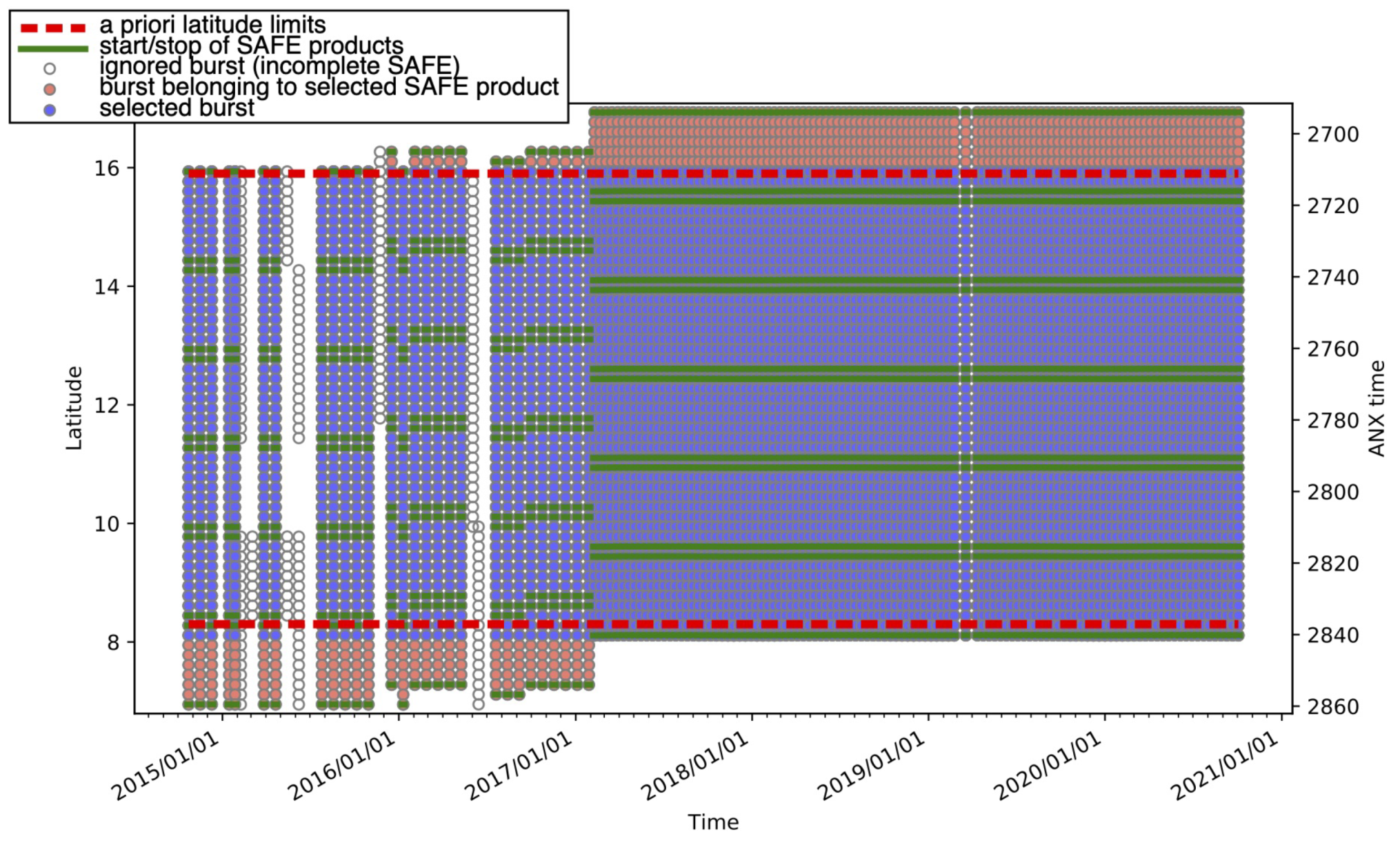
  • Select bursts for each subswath independently and retain only complete acquisitions within the chosen latitude range;
  • Download precise orbits, compute perpendicular, and temporal baselines, and choose a single primary date common for the three subswaths;
  • For each subswath, assemble bursts into Single Look Complex data (SLC), transform the DEM in the primary date radar geometry, and compute the geometrical transformations of all secondary SLCs on the geometry of the primary acquisition, combining orbit, DEM, and correlation offsets information;
  • For each subswath, reassemble secondary SLCs using the position of the burst limits from the primary image and an improved deramping function, and resample secondary SLCs on the primary geometry;
  • Define the interferometric network and computes differential interferograms for each subswath;
  • For each subswath, evaluate spectral diversity parameters and correct interferograms;
  • Merge the subswaths of all interferograms and of some auxiliary images using available metadata and inverted phase jumps in subswath overlaps;
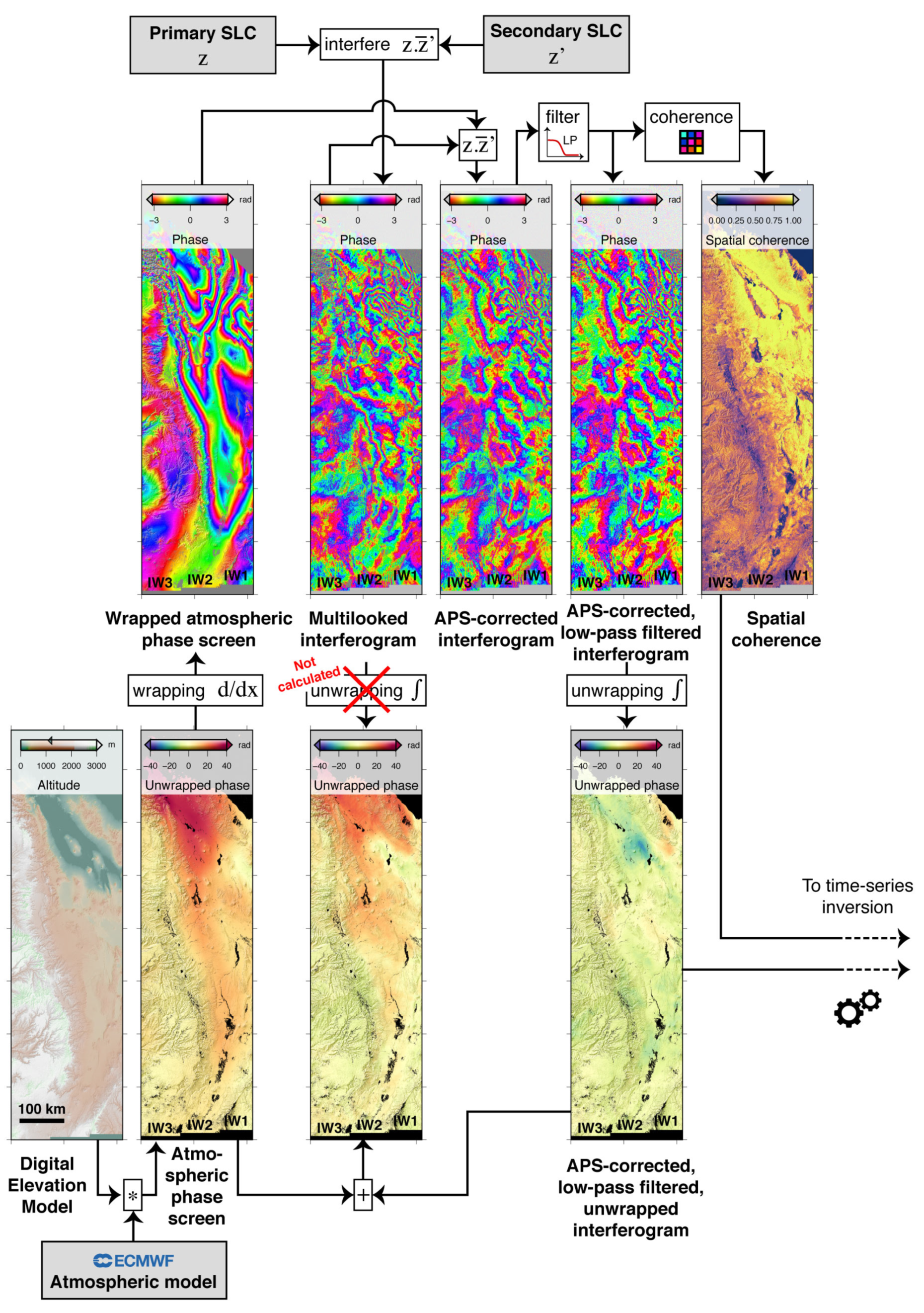
  • Correct interferograms from stratified atmospheric effects, multi-look, filter, unwrap, remove phase ramps in range and azimuth and reference;
  • Discard possible low quality interferograms based on their phase variance or unwrapping fraction;
  • Invert interferograms into time series and provide quality indicators;
  • Prepare products in tiff or geotiff format, together with metadata, previews, and text files.
We detail below a few selected steps, necessary to understand the FLATSIM products.

2.2. Burst Selection

The Sentinel-1 standard acquisition mode (TOPS) consists in sweeping the antenna beam from the aft to the fore, thereby illuminating a portion of the ground called a “burst”. Three sub-swaths are successively covered to broaden the swath. The Sentinel 1-A and 1-B satellites are tasked to maintain synchronicity of burst acquisition, which is essential to ensure an optimal interferometric coherence. However, Sentinel-1 acquisitions do not necessarily cover the same burst coverage. In other words, the acquisition start/stop times (w.r.t., the ascending node crossing time, or ANX time) may vary from one acquisition to another. As input, FLATSIM is given the north and south latitude limits of the area of interest. Then, starting from these a priori limits, an optimization step is required to select the best set of acquisitions that simultaneously maximizes the latitudinal extent of the dataset and the number of acquisitions, without including gaps in the processing. The FLATSIM strategy consists in an iterative search for the optimal number of consecutive bursts that achieves the largest number of complete acquisitions on the chosen set of consecutive bursts (Figure 1). Note that dates of acquisition which are incomplete from one or more of the three sub-swaths are discarded. Up to about 40 contiguous bursts can be selected.

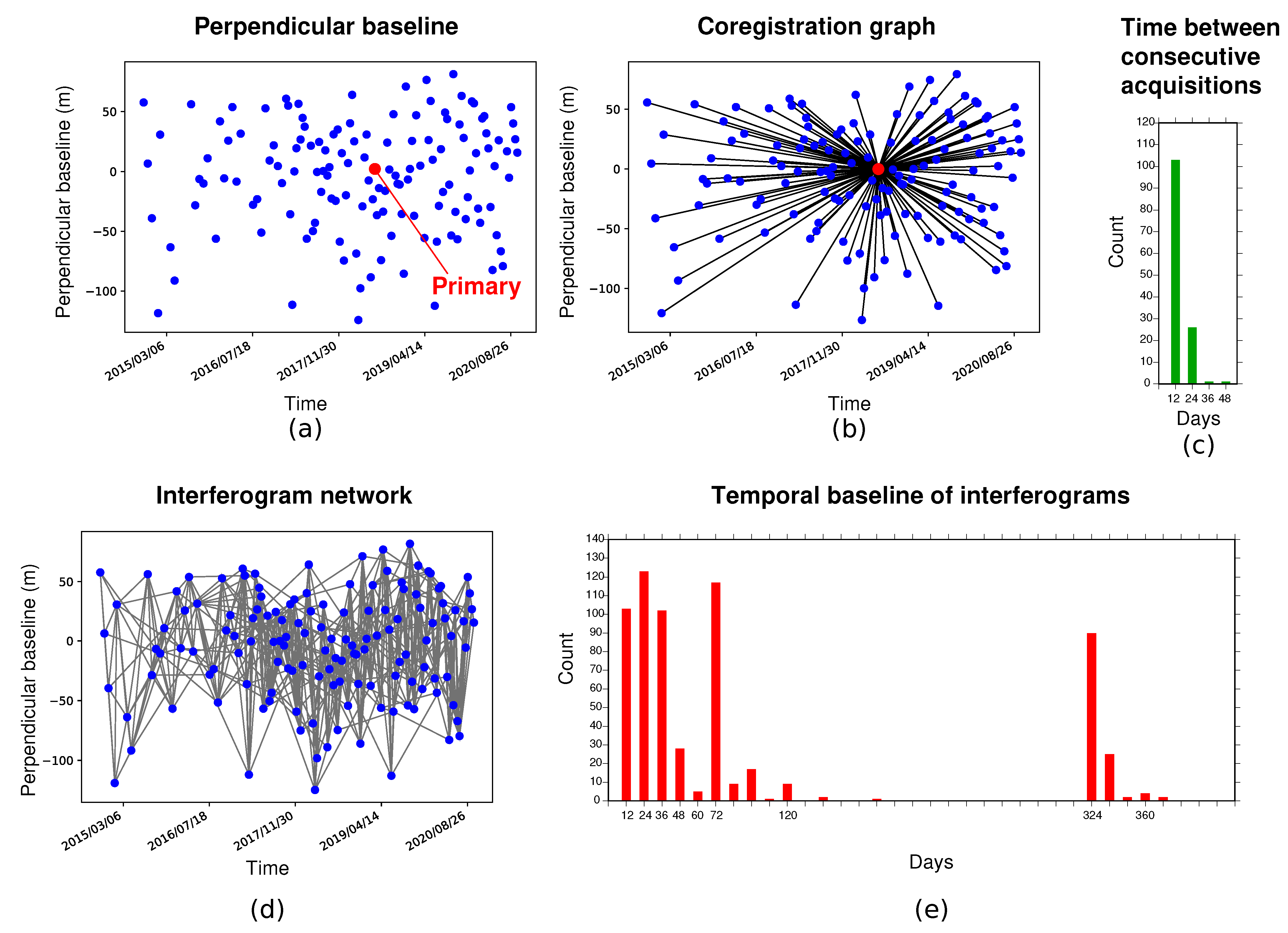
2.3. Coregistration and Interferometric Network Selection

Image correlation is performed between the amplitude image of the primary acquisition and an amplitude image simulated from DEM and orbit information. Found offsets are fitted by a second-order polynomial in range and azimuth. This modeling and further adjustment serve to build lookup tables from radar to ground geometry and vice-versa. We then precisely coregister all secondary images with respect to the primary acquisition (Figure 2, top), as explained in [19]. A simulated topographic phase map (in radar coordinates) is calculated for each of the secondary images, using the precise orbital parameters of the secondary and the primary acquisitions. This simulation is used to predict the distortion in range between secondary and primary images, supplemented by an additional constant offset in range and an affine offset function in azimuth derived from amplitude image matching. The affine offset function depends linearly on range and azimuth. Prior to resampling, a deramping is performed, cancelling most of the azimuthal phase modulation pattern inherited from the TOPS mode pre-processing, taking the azimuth spectral properties of the primary image as a reference for the deramping function and taking into account the affine offset function in azimuth [40].
The chosen network of interferograms includes all n/n + 1, n/n + 2, n/n + 3 couples independently of their perpendicular baselines, and systematic pairs with temporal separation of ~2 to 3 months and ~1 year with restricted perpendicular baselines (Figure 2, bottom). The inclusion of 2 to 3 months and 1 year interferograms is essential for the mitigation of bias due to fading signals [45]. The computed differential interferograms are multi-looked by a factor 8 × 2 in range and azimuth.

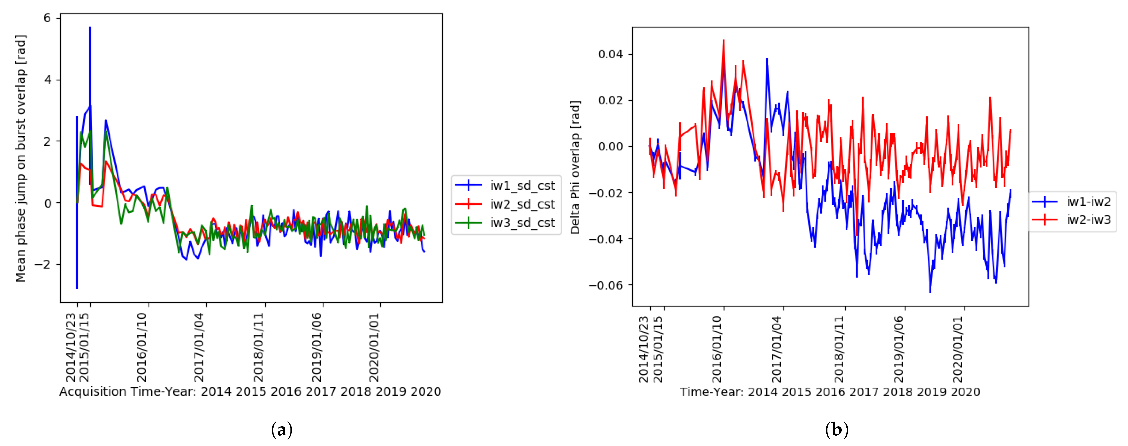
2.4. Enhanced Spectral Diversity Correction

The S-1 TOPSAR default acquisition mode [24] for IW Sentinel-1 data, while enhancing the swath width and then the revisit time, required to adapt the InSAR processing chains to take into account the antenna forward-backward sweeping inside each burst, and the division of the full wide-swath into three overlapping sub-swaths. Slight inaccuracies in azimuth positioning of the images also result in phase jumps across bursts that are accounted for using the enhanced spectral diversity method (ESD, [46]), while subswath merging is facilitated by the accurate timing of subswath SAR SLC as provided before data and a high quality ESD correction.
Here, enhanced spectral diversity is computed on the selected network of interferograms, using forward and backward SLCs of all burst overlaps. The SLCs overlaps are coregistered using the same function as described above, and differential backward-forward interferograms are multi-looked by a factor 64 × 16, using colinearity [47] in the multi-looking operation to enhance the signal to noise ratio. The differential forward-backward wrapped phase screens for all overlaps are then fitted by a four-parameters function: a constant, two linear coefficients describing the range and azimuth change, and a coefficient describing the average linear phase change in azimuth within the bursts. For long tracks, a fifth coefficient, modeling a quadratic phase change across bursts in azimuth was also found necessary. To obtain consistent and stable parameter values for each secondary image, all these parameters, estimated on interferograms, are inverted within the network by a least-squares minimization with outliers removal (Figure 3, left). Using these estimated phase screens, a sawtooth-shaped phase screen is subtracted to the original interferograms to cancel phase jumps across burst boundaries.
The above strategy is applied independently to each sub-swath, and all sub-swaths are then mosaicked, correcting for any phase jumps between the sub-swaths by computing the phase difference in the overlap between sub-swaths, and inverting for these phase differences within the interferometric network (Figure 3, right).

2.5. Stratified Atmospheric Correction

The final steps are performed on the mosaicked interferograms. The atmospheric phase screen of interferograms can be divided into a pseudo stratified contribution, that is at first-order dependent upon elevation, and a more random contribution often named “turbulent”. The dry and wet stratified atmospheric delays, that derive from the temporal variations of the layered atmospheric variables (pressure, P, temperature, T, humidity, q), can be easily predicted from global atmospheric models with the assumption of a mainly horizontally layered atmosphere [48,49]. The turbulent contribution is difficult to model from independent atmospheric information as it requires to place the atmospheric patterns at the right place in space and time.
In the FLATSIM service, the stratified atmospheric phase screen is computed in 8 × 2-looks using the geopotential height of pressure levels, and T and q given for each of the 37 pressure levels by the European Centre for Medium-Range Weather Forecasts (ECMWF) ERA-5 meteorological reanalysis [50]. The delay is first interpolated as a function of elevation with a very fine vertical spacing at regularly spaced ERA-5 nodes (every 0.25 degree). Then, for each pixel in radar coordinate, characterized by its elevation, latitude, longitude, and look angle given in separate grids, we compute the delay by bilinear interpolation of the surrounding four ERA-5 nodes. This procedure is very efficient and easily parallelized.
In addition to an elevation dependent contribution, the stratified APS also includes large-scale phase delay gradients along range and azimuth. The correction before unwrapping (e.g., [51]) strongly reduces fringe rates in areas of high relief (Figure 4). The ERA-5 model, given with a temporal sampling of one hour, is found more accurate than other global atmospheric models (e.g., the high resolution global analysis of ECMWF, given every six hours). However, the ERA-5 modeled surface elevation is a smooth surface that stands above deeply incised valleys. As a result, the phase delay as a function elevation below the smooth surface is an extrapolation that is not very well constrained.

2.6. Interferogram Multi-Looking, Filtering, and Unwrapping

After atmospheric correction, we take further looks to obtain 64 × 16 or 32 × 8 looks interferograms (this choice, fixed for a given region of interest, is left to the PIs of the scientific proposals). Filtering is performed by averaging on a 12 × 12 triangular sliding windows weighted by spatial coherence.
Unwrapping of multi-looked interferograms uses the coherence associated to the filter averaging process on complex values to guide the unwrapping integration path [19,51]. The unwrapping path is also set to avoid crossing large topographic gradients in radar geometry. Its seed point is automatically chosen in an area with good coherence over the interferogram stack. These choices for the filtering and unwrapping procedure are quite suitable for an automatic processing over mountainous and vegetated areas with limited displacement gradients, but is not adapted to large deformation gradients.
After unwrapping, coefficients of a linear phase ramp in range and azimuth are computed for each interferogram, together with the residual phase standard deviation. The coefficients are inverted over the interferometric network in order to get a consistent flattening of each interferogram. The phase standard deviation is also inverted for each time step, as in [18]. All interferograms are referenced by setting the averaged phase in a small area adjacent to the unwrapping seed point to zero.
Finally, the unwrapping fraction (proportion of the pixels unwrapped in one interferogram), the residual phase standard deviation per interferogram and the residual phase standard deviation per date are used to automatically discard anomalous interferograms or anomalous acquisitions. This step is very important in the automated FLATSIM procedure to ensure the quality of the final products. It typically discards from 0 to 20 interferograms and 0 to 3 acquisitions per processed track (see Figure 5).

2.7. Time Series Inversion

The time-series inversion of the line-of-sight displacement follows the principle described in [18,19,52], and depicted in Figure 6. We jointly solve for both the total phase delay time series and a temporally smoothed time series. The first one, delivered by FLATSIM, includes both line of sight (LOS) displacement and residual atmospheric phase screen, whereas the second, for which temporal fluctuations at short time scales induced by atmospheric turbulence are filtered out, only serves as a regularization, in case we get disconnected data subsets in the unwrapped interferograms network. Unwrapping errors are corrected iteratively, by searching for the optimal integer number of phase cycles to be added in areas detected as incorrectly unwrapped. For this step, the correction is prioritized on interferograms characterized by a large residual between the initial and reconstructed line-of-sight displacement maps. After a few iterations, the root mean square misclosure map is computed for the whole dataset, together with a root mean square misclosure for each interferogram, and for each acquisition [52]. Using the total phase delay maps at each time step, an average LOS velocity map is calculated by a simple pixel-by-pixel linear least-square regression in the temporal dimension. The velocity map is then slightly improved by iteratively reducing the weight of the acquisitions with large deviations from the trend of the mean displacement.

3. FLATSIM Architecture

The goal of the FLATSIM project was to integrate the NSBAS chain in the CNES high performance computing (HPC) infrastructure to benefit from its computing power and from the fact that CNES mirrors locally the Sentinel-1 data from ESA. FLATSIM is thus able to process up to 6 years of Sentinel-1 data over large geographical areas (up to 7 million km2 per year in total). FLATSIM is designed to automatically access and process Sentinel-1 radar images and to distribute interferometric products which cover worldwide areas of interest. As shown in Figure 7, FLATSIM is composed of two main components: a production module and a delivery module.

3.1. Architecture of the FLATSIM Project: Distributed and Scalable by Design

The strategy behind the integration of NSBAS in the FLATSIM project was to make NSBAS processing massively parallel. Even if most of its steps can be run in a parallel way, NSBAS was conceived as a global processing chain running on a single-node, monolithic workspace, in which all the data generated during the NSBAS workflow are stored, from acquisition of the Sentinel-1 single look complex (SLC), to production of the time-series and formatting of distributed data. The integration of NSBAS in FLATSIM is based on a different logic, that consists in splitting the NSBAS chain in a set of unitary processes for which the inputs and outputs are clearly identified and cataloged. This way, it is possible to create for each unitary process its own workspace, from the cataloged data, including only the data necessary for its execution. It then becomes easier to dispatch these treatments on the computing resources.

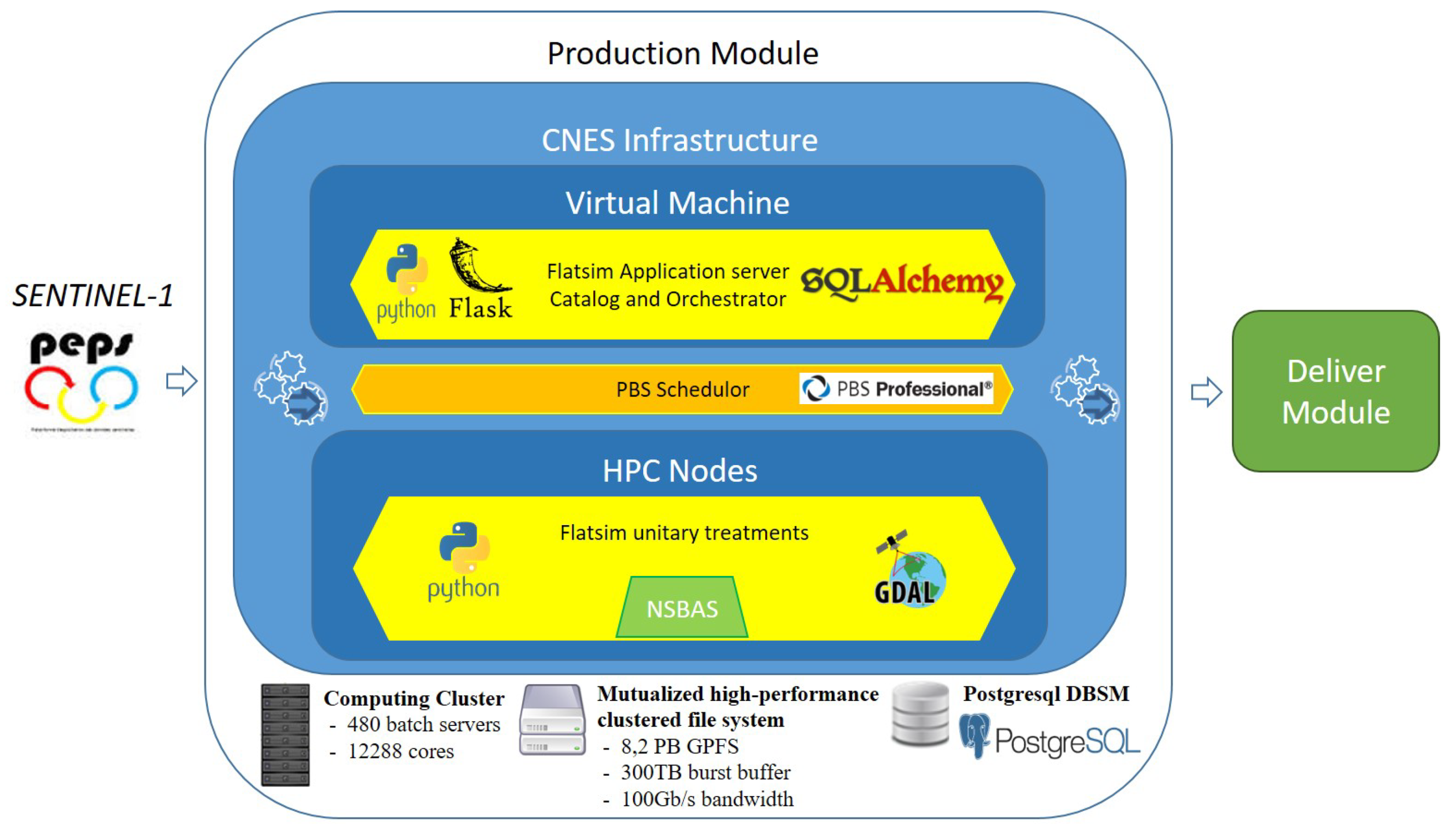
3.2. Architecture of the CNES HPC Infrastructure

The CNES HPC infrastructure is a shared facility at the disposal of CNES projects and partners. It is composed of more than 480 batch servers for a total of 12,288 cores (725 Tflops) and a 8.2 PB general parallel file system (GPFS) with 300 TB burst buffer offering a bandwidth up to 100 GB/s. This large computing capacity should enable FLATSIM to meet its production objectives. The integration of NSBAS should also be optimized to the CNES HPC, to avoid FLATSIM deteriorating the level of service for all the other users of this computing center.
FLATSIM also relies on various services offered by CNES computing division, such as different types of data storage, database management system (DBMS) hosting services, and website hosting mutualized services.

3.3. Architecture of the FLATSIM Production Module

The technical environment of the production module includes the HPC and the GPFS, a shared PostgreSQL
DBMS, and the mutualized datalake (composed of several data storage spaces). The architecture of the production module (Figure 8) is based on 2 sub-components:
  • The FLATSIM application server which includes catalog and orchestrator capabilities;
  • The FLATSIM unitary treatments that integrate NSBAS as a library and run as unitary jobs on nodes of the HPC center.
The FLATSIM application is in charge of referencing data, orchestrating processing steps and submitting them as unitary jobs to the scheduler. The data cataloged by the application server are stored on the GPFS, while their metadata and status of processing steps’ jobs are registered in the PostgreSQL database.
Through the integration, each step of the NSBAS workflow has been divided into unitary processes, which can be performed in isolation and parallel for each unique data (SLC or interferograms) in different jobs spread on the HPC’s nodes. During their execution, a job’s temporary data are written on the local storage of the node, and, at the end of the execution, output data are transferred and cataloged by the FLATSIM application server, to be used as input of the next step jobs. Once the output data are cataloged, the job also updates its status in the application server.
The FLATSIM application server is also responsible for the processing sequencing. It monitors the production status of each step, and when one step is completed, based on its parametrization, its internal logic, and the data cataloged, it identifies the jobs to process for the next step, and submit these new jobs to the distributed resource manager (DRM) PBS-PRO, that will dispatch them on the HPC nodes. At any time during the production, the operators can interrogate the FLATSIM application server to request information on the production status, and act on products or jobs if necessary.
During the first step of the production, FLATSIM gets SENTINEL-1 Level-1C products via direct privileged access on the PEPS platform (developed by CNES in the context of collaborative ground segments of Copernicus program) and stores them in the application server catalog. After the packaging step, the FLATSIM output products are transferred on the mutualized datalake, which is accessible by both the production module and the delivery module. At the same time, these products metadata are sent to the delivery module to be registered in its database.
By default, the scheduling system in the CNES HPC allows a project to submit jobs on up to 800 cluster cores. Under these conditions, processing a Sentinel-1 swath covering 5.5 degrees of latitude to generate a 8 looks resolution (about 100 m pixel size) time series over 5 years’ time depth requires approximately 10,000 h of CPU time and 60 h of real time.

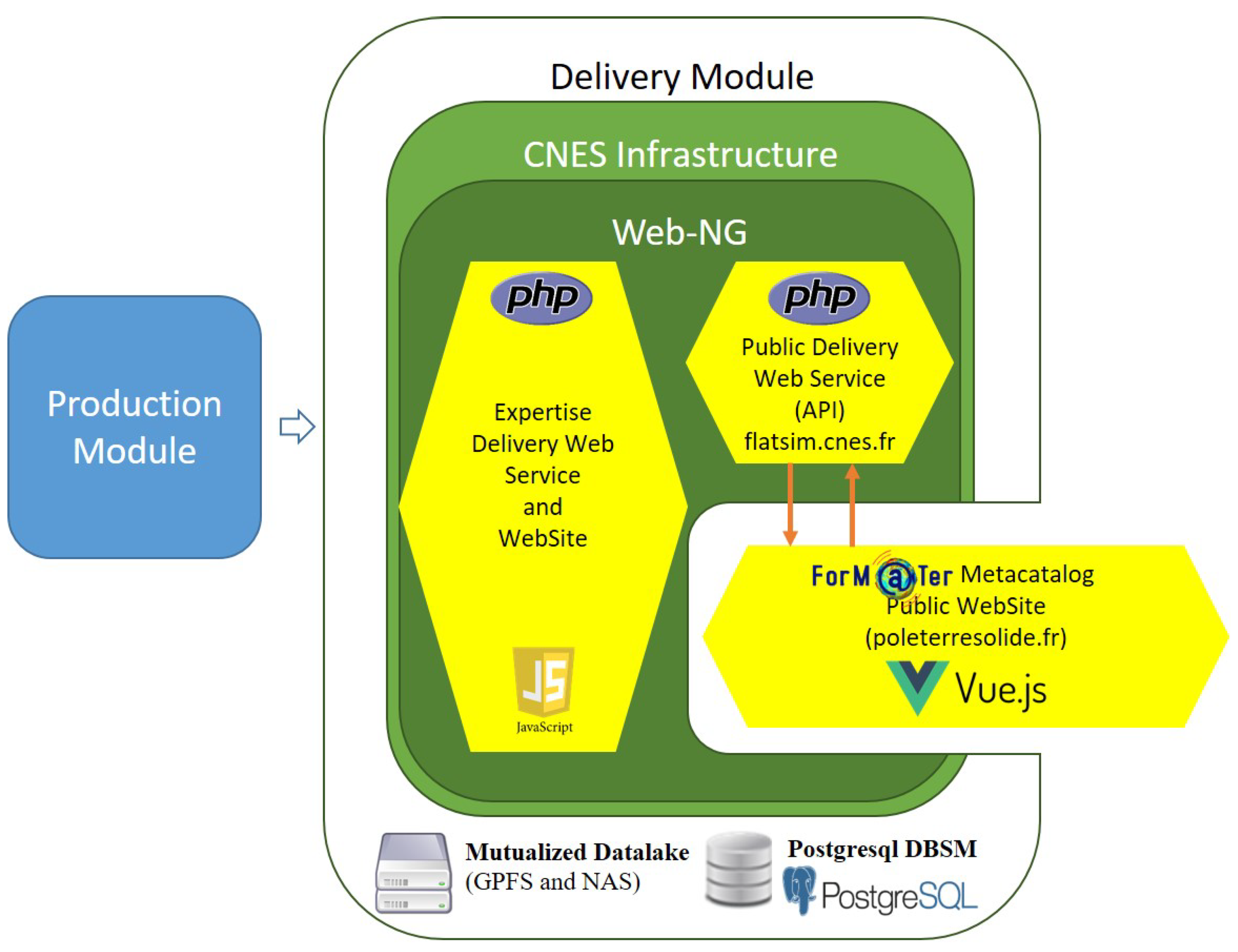
3.4. Architecture of the FLATSIM Delivery Module

The role of the delivery module (see Figure 9) is to diffuse the FLATSIM products to the scientists and public community. The products are first made available to scientific experts for validation before being distributed to end users.
The FLATSIM delivery module is composed of web services and websites. The web services and the expertise website are packed in an Apache HTTP server hosted in the CNES infrastructure in a virtual machine (VM) provided by the CNES web-site hosting mutualized services called Web-NG. In the CNES infrastructure, the delivery module uses a shared PostgreSQL DBMS and the mutualized datalake to store the data. Depending on their types, the data are stored on different technical means:
  • Downloadable products on the GPFS part of the datalake;
  • Visualization data on the network attached storage (NAS) part of the datalake;
  • Metadata in the PostgreSQL database.

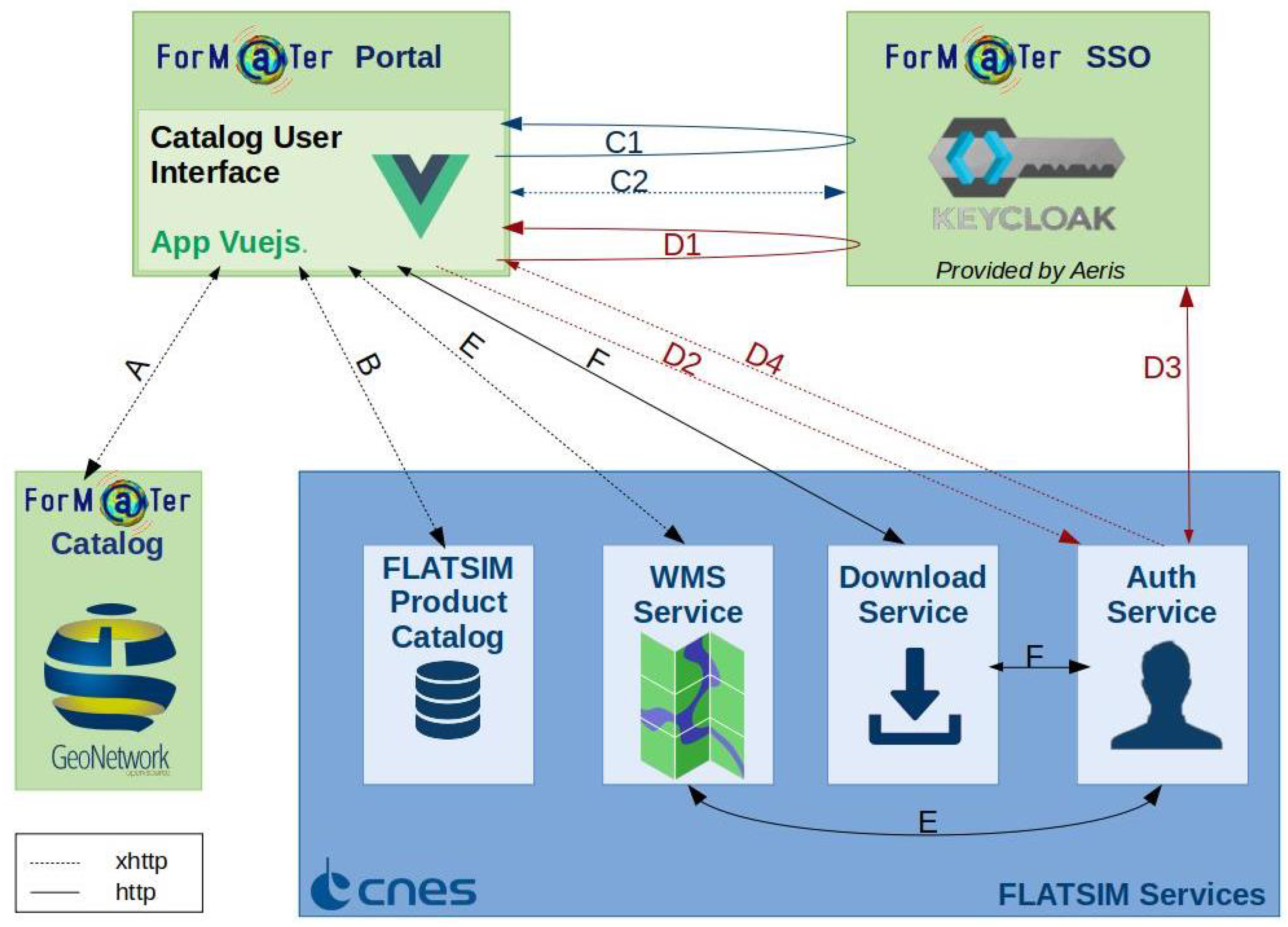
3.5. User Access Interface

The public data access is made via the ForM@Ter website, on the “Terre Solide” metacatalog page (https://www.poleterresolide.fr/, accessed on 10 September 2021), which is a Vuejs (javascript) application embedded on a page of a Wordpress site. The CNES public delivery web service provides an Opensearch Application Programming Interface (API) which allows access to the catalog of distributed products. The metadata of the FLATSIM collections (for each study area) are recorded by the ForM@Ter meta-catalog in a Geonetwork catalog under the ISO19139 standard. Downloading and viewing products with warehouse management system (WMS) is reserved for authenticated ForM@Ter users. Authentication is done with the ForM@Ter single sign-on (SSO).
In Figure 10, we display the requests made at the interface between the ForM@ter portal, the ForM@ter SSO, the Form@ter catalog, and the CNES FLATSIM services:
  • Request A: Geonetwork’s Q Search API is used for user searches among collections. These searches can be spatial, temporal, by data center, open term, variable, or platform. The requests are xhttp requests, invisible to the user;
  • Request B: The meta-catalog‘s Opensearch API allows searches among the granules of a FLATSIM collection. The requests are xhttp requests, invisible to the user;
  • Requests C1 and C2 (User authentication for the metacatalog):
    • C1, the user authenticates with the Keycloack SSO and is redirected with a code to the meta-catalog page;
    • C2, the Vuejs meta-catalog application queries the SSO with the code to obtain an access token and user information (invisible to the user),
  • Requests D1 to D4 (Authentication with FLATSIM):
    • D1, the user authorizes FLATSIM to access his user data and is redirected to the meta-catalog page with a code for FLATSIM authentication;
    • D2, the meta-catalog application transmits the code to the FLATSIM authentication service (invisible to the user);
    • D3, FLATSIM’s authentication service queries the SSO with the code, to get user data (invisible to the user);
    • D4, the authentication service transmits a FLATSIM data access token to the meta-catalog application (invisible to the user);
  • Request E: The user now has a FLATSIM access token, he can query the WMS Flatsim service by transmitting the token. The service checks that the token is valid with the FLATSIM authentication service and sends the images back (invisible to the user).
  • Request F: The user now can request a download by transmitting the token. The service checks that the token is valid with the FLATSIM authentication service and then returns the archive (invisible to the user).

3.6. Service Access

Processed areas are selected through a series of call for research proposals, with an independent committee evaluating the scientific objectives, feasibility, and team skills, bearing in mind that the amount of square kilometer processed per year is limited. This call is currently dedicated to the French scientific community. Products are freely available for the French scientific community. The international community will access the final displacement rate maps (after thorough validation, possible partial reprocessing, tying up to geodetic reference frame, and a first data analysis by scientific teams) through peer-reviewed publications with a reference to the FLATSIM service.

4. Description of Products

4.1. General Description

The choice of the number of products and their processing level delivered by the FLATSIM service was a trade-off between providing only a few small-size high-level products ready-to-use for users non-expert in InSAR and providing the huge amount of all intermediate and final products along with processing logs, most of which are only potentially useful to user experimented in InSAR processing and require large storage and download capabilities on both the provider and user sides.
Compared to other MTInSAR services, such as LicSAR or P-SBAS on GEP, we have chosen to put the slider more on the side of a rather large product set giving great flexibility for post-processing and analysis of results. This choice results from our long InSAR processing experience showing that starting from the coregistered stack of wrapped interferograms (that is a large burden of the processing) some processing steps can be optimized a-posteriori based on the analysis of the first time-series results.
The details of the products made available by FLATSIM are described here: https://formater.pages.in2p3.fr/flatsim/ (accessed on 10 September 2021). Here, we give insights on the main types of products that are delivered, including quality assessment products and auxiliary products useful for controlling how successfully the automated workflow proceeded. Except for the DEM which is provided only in radar geometry, all the products are delivered in both radar and ground geometries. For instance, this allows the user to re-run with his own computing resources the unwrapping step, or the time series inversion, before geocoding. We give all the necessary information so that the user can redo the processing from the merged, 2-looks, wrapped interferograms, if needed.
The products are delivered separately for each processed track as three types of packages: interferogram, time-series, and auxiliary data. Filenames are formed according to the following naming convention:
 
CNES_TYPE_GEOMETRY_[DATE1_DATE2]_LOOKSrlks.EXT
 
in which
TYPE 
points toward the file type (i.e., wrapped interferograms, coherence, etc.). See hereafter for a more detailed description.
GEOMETRY 
is set either to radar for radar geometry or geo for ground geometry.
DATE1 
(DATE2, respectively). These optional fields corresponds to the date at which the first (second or last, respectively) image has been taken.
LOOKS 
is the number of looks used to downsample the image (note there is a factor 4 between the number of range and azimuth looks, i.e., 2 looks means 8 looks in range and 2 looks in azimuth).
EXT 
is the extension of the file that defines its type:
tiff 
contains the data;
png 
a preview file. It comes with a legend file, typically a colorbar with the scale information.
meta 
a file that contains additional metadata. It contains for example information about the parameters of the processing chain, or about the product itself like its DOI, or about the satellite geometry, like the orbit direction, the relative orbit number, etc.
In each package, in addition to the main products, previews, graphs and small text files that contains statistics allow a quick quality assessment of different processing steps. The size of large products is also given in the next subsections. Although some files can be particularly large (>10 Gbytes), Geospatial Data Abstraction Library (GDAL) or GDAL API for example can easily manipulate them and extract sub-grids with lower spatial or temporal resolution. These sub-grids can be used in data analysis packages performing, for example, principal or independent component analysis, if these packages have data size limitations.

4.2. Packages of Interferogram Products

There is one package per interferogram. It contains a set of files related to a given interferogram that are synthesized in Table 1.
  • Wrapped/Unwrapped Interferogram
    InW (InU, respectively) is the wrapped (unwrapped, respectively) merged interferogram. Wrapped interferograms in radar geometry are provided both in 2 and 8 (or 16) looks. The initial number of looks of the interferograms before they are geocoded is given in their names and metadata. The ground pixel spacing is chosen according to the initial pixel spacing in radar geometry. The InWF and InU products are spatially filtered. All interferograms have been corrected using spectral diversity and the ERA5 atmospheric model.
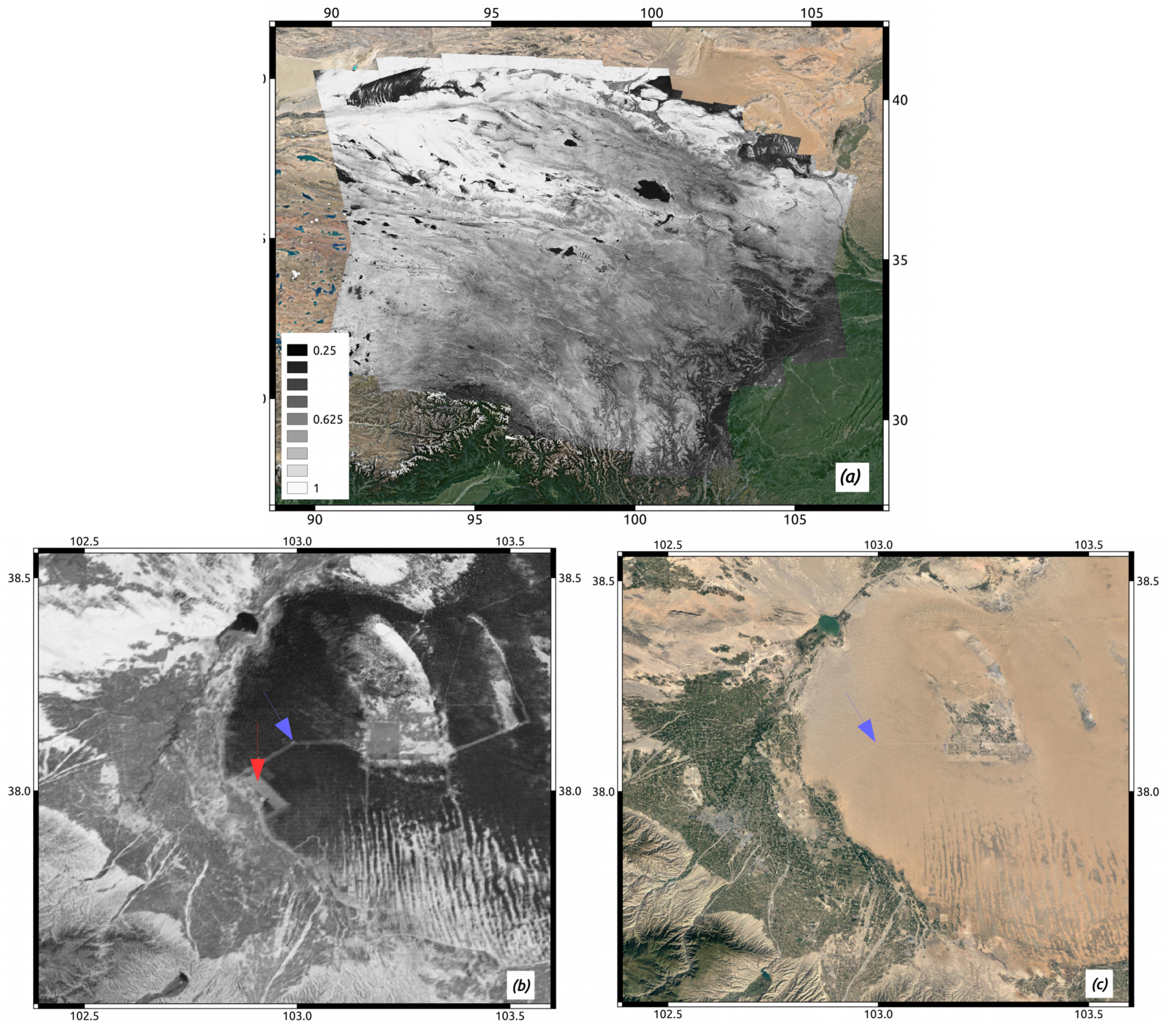
  • Spatial coherence
    Coh is the spatial coherence of the wrapped interferogram. It can thus be considered as a proxy of the quality and reliability of the signal. Typically, the spatial coherence will be very low (close to zero) at points located on water—e.g., sea, lakes, rivers, snow—and close to one at locations with stable backscattering properties where there is no vegetation—e.g., deserts, rocky mountains without snow, roads, buildings, etc.
  • Atmospheric phase screen
    APS is the phase delay induced by the atmosphere as predicted by the ERA-5 atmospheric model [50] and mapped on the DEM [48,49].
Each zipped interferogram package is about 2.2 Gb for 25 processed consecutive bursts (450 km long segment). This large size is partly due to the interferogram product in 2 looks and in radar geometry (i.e., with a spatial resolution of about 30 m, 1.3 Gb), whereas 8-looks interferograms, APS or coherence maps in ground geometry (pixel spacing of 0.00111 degree, 124 Mb) and in radar geometry (resolution of 120 m, 82 Mb) are less heavy.

4.3. Time-Series Package
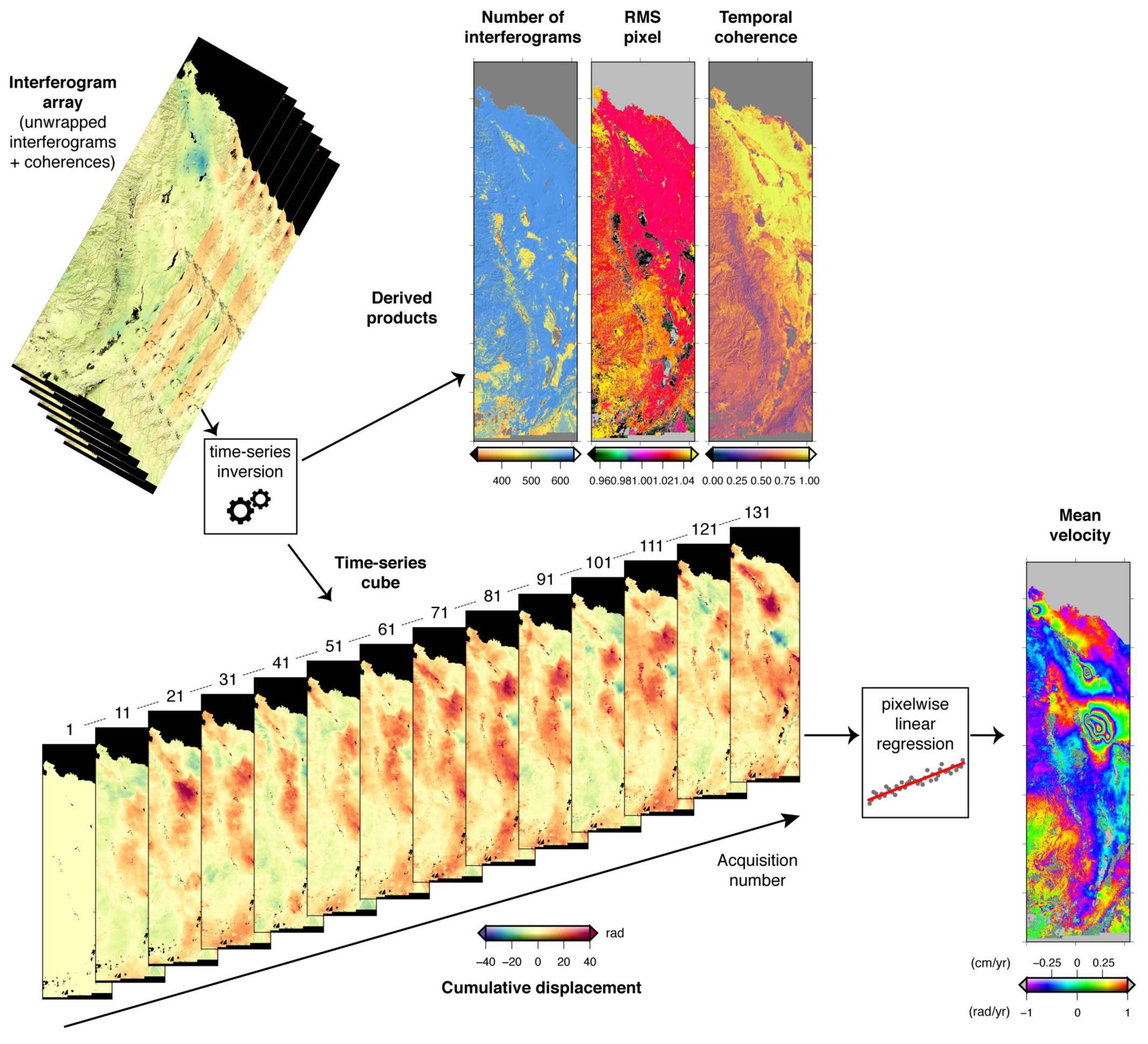
This package corresponds to products generated at the time series inversion step (see Section 2.7). Map products are given in 8 (or 16) looks, in radar geometry and in ground geometry. Table 2 summarizes the time series products.
  • DTs: time-series
    This product is a data cube that contains the cumulated total phase delay images at each acquisition with respect to the first date. In practice, the reference is set to the origin of a linear fit through the time series for each pixel. This representation avoids for the APS of the first image to appear in negative on all other dates. Note, however, that it is not ideal in case of strongly non-linear deformation. The time series may be incomplete for some pixels and for some dates, and values are then replaced by NaN. We choose to deliver the total phase delay, that includes both residual atmospheric phase screens and displacement signals, without any attempt by us to separate both contributions. This allows the user to perform its own separation, possibly guided by his knowledge of the expected deformation signal properties.
    The geotiff file includes as many bands as time steps. The unit is in radians along LOS, positive away from satellite. Each band is named by the acquisition date. The associated preview file displays the cumulated displacement at the last time step.
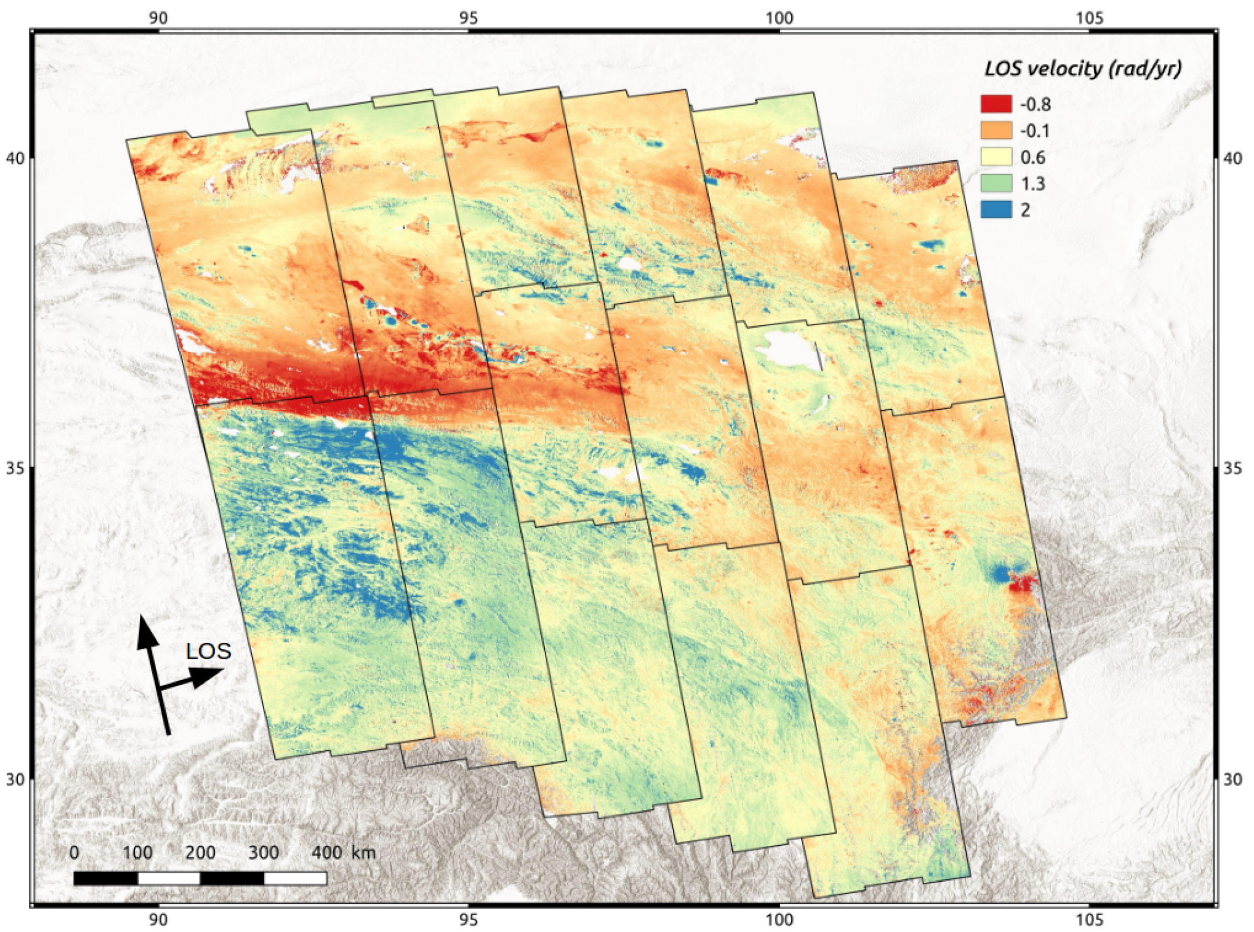
  • MV-LOS: LOS velocity
    The mean LOS velocity is given in a geotiff product with two bands:
    Band 1 is the mean velocity in rad/yr, positive away from satellite;
    Band 2 is a shaded view of the topography, with an illumination simulated to match the radar backscatter amplitude.
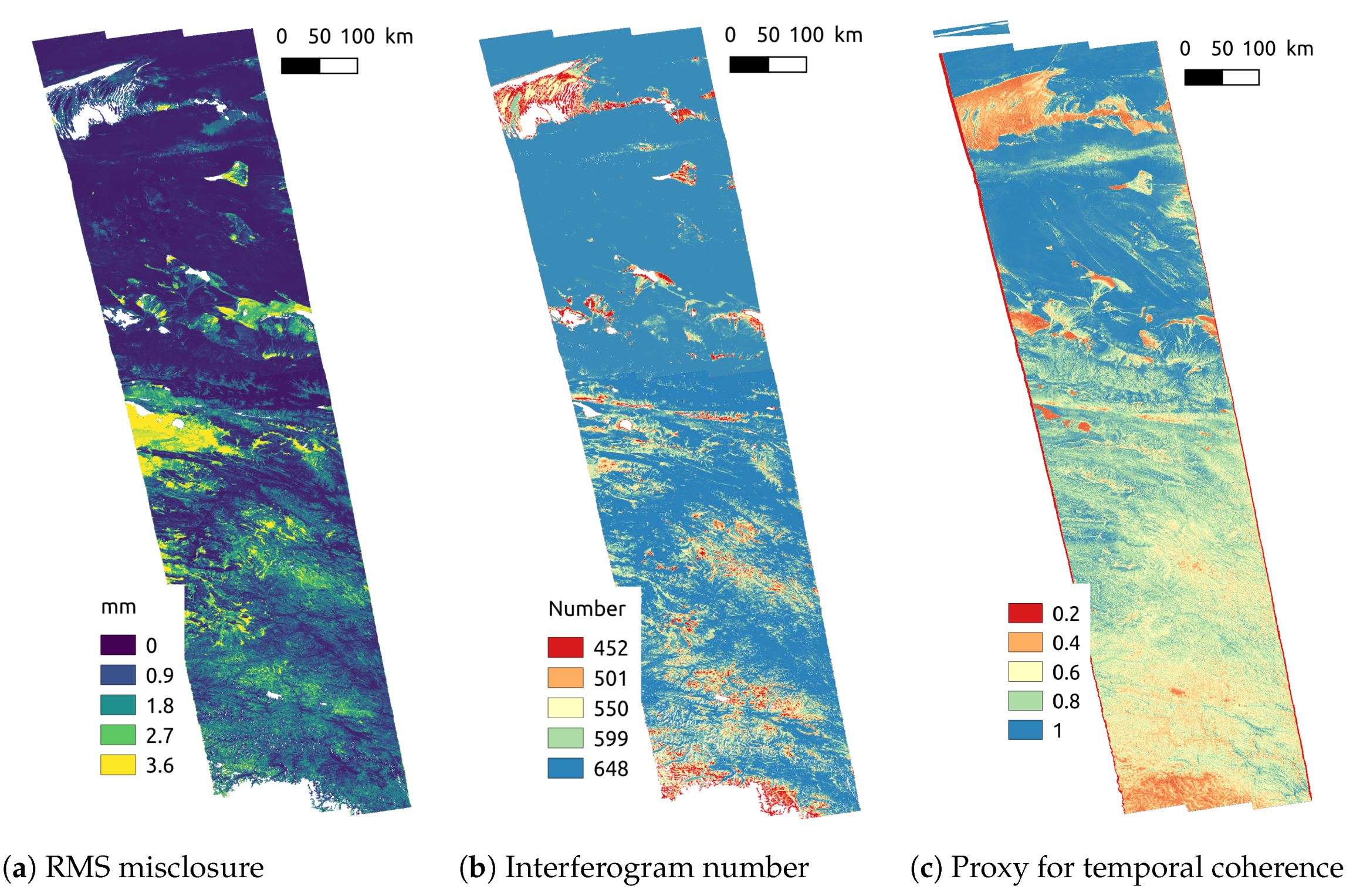
  • Net: Quality assessment product
    This geotiff product gives various indicators of the quality of the time series inversion, provided in radar and in ground geometry.
    Band 1: RMS misclosure of the interferogram network for each pixel, in rad;
    Band 2: Number of interferograms used in the time series inversion for each pixel;
    Band 3: Number of images used in the time series inversion for each pixel;
    Band 4: Proxy for the temporal coherence, computed as the norm of the average of all successive interferometric triplets (between 0 and 1);
    Band 5: Proxy for a possible bias in the timeseries, computed as the argument of the average of all successive interferometric triplets (in rad).
  • Stk-In: interferogram list product
    It gives information on the timeseries, as for example the list of dates and interferograms used as input to the time serie inversion and the reference image that was selected.
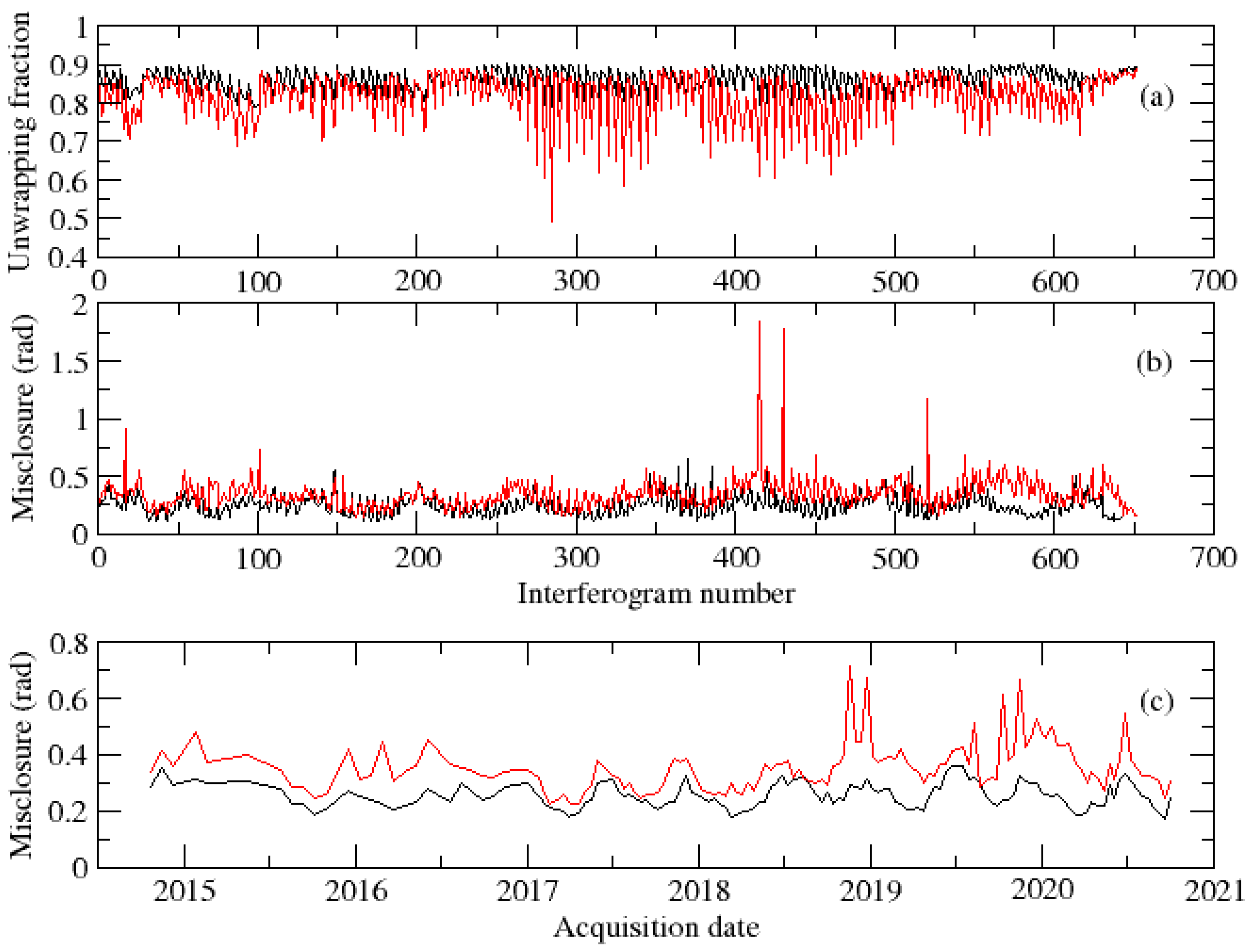
  • Additional txt files
    The “RMSinterfero.txt” and “RMSdate.txt” files, together with their png previews, are very useful to check possible problems on interferograms or on acquisitions. They provide the RMS interferometric network misclosure averaged either by interferogram or by date. For example, the RMS value for some interferograms will be large in case of uncorrected unwrapping errors. Specific errors associated with one image, for example in case of snow, strong atmospheric or ionospheric perturbations, or bad azimuth frequency modulation corrections, can also be detected.
The zipped time-series package is about 6.7 Gb for 25 processed consecutive bursts (450 km long segment) and 100 processed images. The package size will increase linearly with the number of processed bursts and images. The data cube has a larger size in ground geometry (6.1 Gb, pixel spacing of 0.00111 degree) than in radar geometry (4.1 G, resolution of about 120 m).

4.4. Auxiliary Data Package

This set of products (Table 3) provides the user with auxiliary information common to the whole dataset, including look-up tables (LuT), LOS unit vectors, and processing parameters, etc.
  • CosENU: LOS unit vector
    The three-bands geotiff product in either radar or ground geometry gives the LOS unit vector u = ( u E , u N , u U ) , along the satellite to ground direction, such that the LOS velocity, V L O S , can be related to the ground velocity vector, V = ( V E , V N , V U ) , by V L O S = V E u E + V N u N + V U u U
  • LuT: Look-up tables
    The provided LuT tables allows to project 2-looks or 8-looks products in radar geometry in ground geometry and inversely.
  • TCoh: Radar backscatter properties
    This product assembles at about 40 m × 40 m resolution backscatter properties averaged over the complete data stack. It includes (1) the averaged SLC amplitude, (2) the amplitude dispersion index ( σ A / A ¯ , (3) the norm of the complex average of all successive interferogram triplets, (4) the argument of the complex average of all successive interferogram triplets.
  • Auxiliary text files
    Numerous text files are added in the package for users wanting to verify some crucial processing steps. They include perpendicular baseline information, parameters for enhanced spectral diversity corrections for each sub-swath, interferogram unwrapping fractions, and interferogram phase standard deviations.
The zipped auxiliary package is about 11 Gb for 25 processed consecutive bursts (450 km long segment). The package size will increase linearly with the number of processed bursts. The largest product sizes are for auxiliary information in 2-looks. LuT in 2-looks have a size of 2.2 Gb in ground geometry (pixel spacing of 0.000277 degree) and of 1.3 Gb in radar geometry (resolution of 30 m). They allow to geocode the wrapped 2-looks interferograms. The TCoh product is larger in ground geometry (3.9 Gb, pixel spacing of 0.000277 degree) than in radar geometry (2.6 Gb, resolution of 30 m). The LOS unit vector in 2 looks is only given in radar geometry (2.0 Gb), whereas in 8-looks it is only 186 Mb in ground geometry and 123 Mb in radar geometry.

5. Results and Products Qualification

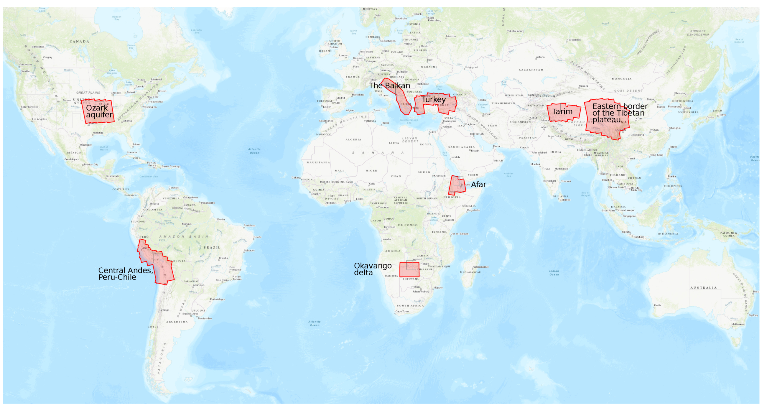
5.1. First Processed Areas

In May 2020, a first call for proposals was open to the French scientific community to identify priority regions for FLATSIM processing. Figure 11 presents all the regions of interest retained for this first call. Nine projects were selected covering different scientific interests. An InSAR expert from the FLATSIM project was attributed to each project. The role of this expert is to interact beforehand with the user to define the key processing parameters. At the end of the processing, the expert helps the user to assess the quality of the generated products.
  • The Ozark aquifer project covers a region located in North America. It focuses on the study of the deformations associated with the Ozark aquifer (south of the Mississippi basin), subject to strong variations in groundwater level, and in neighboring regions where significant seismicity is observed, with a strong seasonal component (New Madrid), or related to wastewater injections (Oklahoma). The objective is to better understand the geodetic signature of the hydrological cycle;
  • The Central Andes, Peru–Chile project aims at (1) better understanding the seismic cycle of the Andean subduction zone in Peru and Chile and of the crustal faults in the Andes, (2) monitoring the dynamics of the large active volcanoes in the region (and to detect possible precursors to eruptions), and (3) at studying the seismic, climatic, and anthropogenic forcing on the dynamics of landslides in the Andes;
  • The Balkan region is one of the most seismically active zones in Europe, with intense industrial and demographic development. The purpose of the project is to better quantify the deformations of tectonic origin in this region (kinematics and localization of active faults, study of earthquakes). It also aims at quantifying the deformations of anthropogenic or climatic origin (linked to the exploitation of natural ressources or to variations in sea level);
  • Turkey: The objective of this project is to characterize the seismic and aseismic behavior of the North Anatolian and East Anatolian faults, in order to better assess their seismic hazard and understand the physical processes governing the dynamics of a fault. It also includes the monitoring of deformations in the grabens of western Turkey, which are major geological structures with high seismic potential;
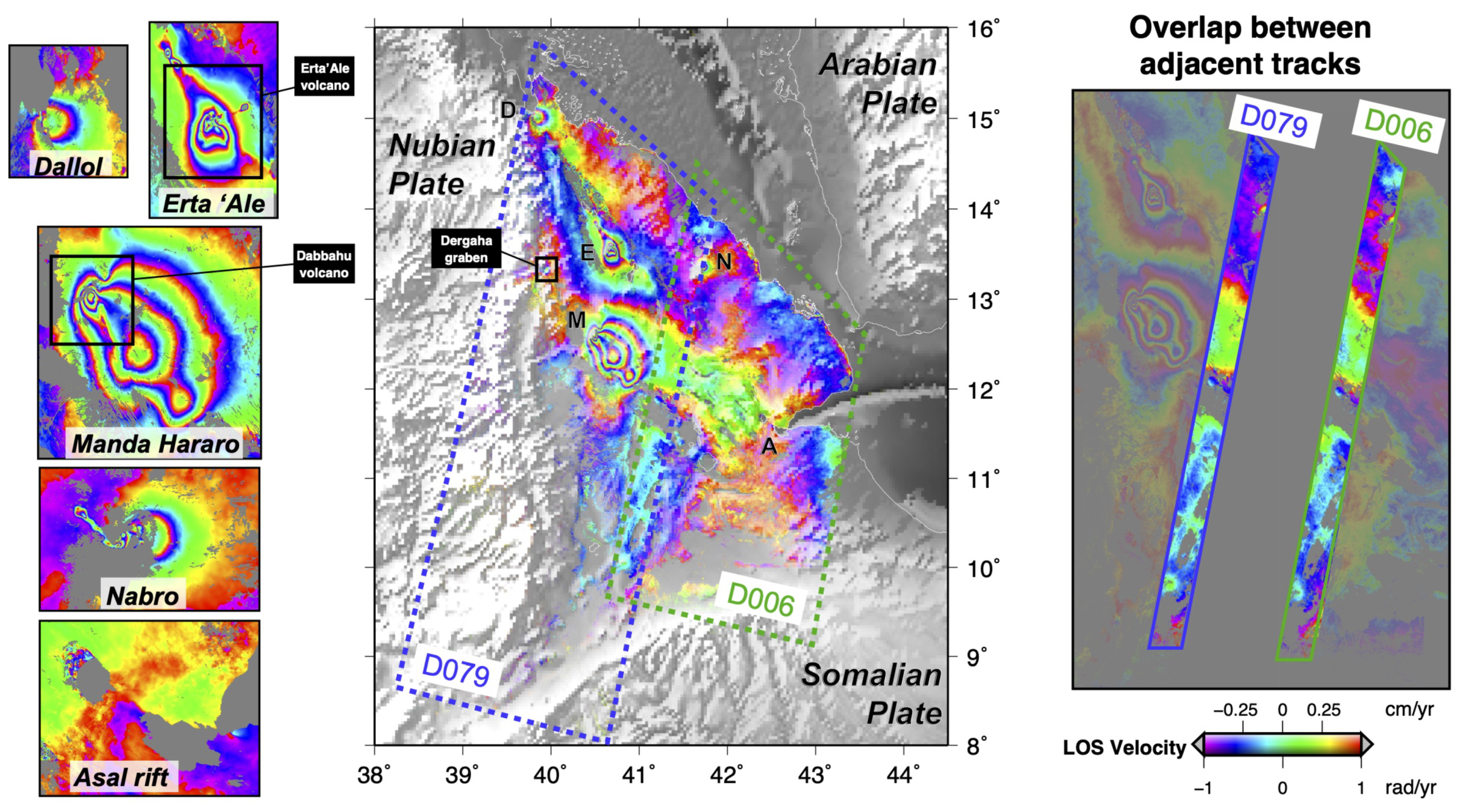
  • The Afar project aims at characterizing the spatial and temporal distribution of the deformation in the region of the Afar depression. The purpose is to better understand the large-scale tectonics (localization of divergent borders, kinematics of the triple point), but also the dynamics of volcanic, seismic, and aseismic events, and the mechanics of active faults. The issue of landslides hazard will also be addressed;
  • Okavango delta: This project aims at better understanding the deformations of tectonic origin in the area of the Okavango Delta (associated with the functioning of the Okavango rift and the East African rift), or of hydrological origin (linked in particular to the flood cycle), and the possible interactions between tectonics and hydrology in this region;
  • The Tarim project focuses on the analysis of tectonic deformations along the Western Kunlun Range, on the northwestern edge of the Tibetan Plateau. This region is marked by the interaction between large strike-slip and thrust faults, with in particular the existence of one of the largest thrust sheet in the world, whose interseismic loading and capability to produce “mega-earthquakes” will be investigated;
  • Eastern border of the Tibetan plateau: The objective of the project is to quantify and model the current deformations on the eastern edge of the Tibetan plateau. It focuses on deformations of tectonic origin, at the scale of active faults, as well as at the continental scale, to address issues of the seismic cycle and uplift mechanisms of the Tibetan plateau. This project is also interested in monitoring non-tectonic signals present in the time series (hydrological overloads in particular).
In the following sections, the Afar and the Tibetan case studies will be taken as examples to illustrate the processing results and the quality of the products of the FLATSIM-NSBAS processing chain (Figure 12). For Tibet, we will display the results of a very long track, A070, from the Tarim basin to the North down to the southern part of Tibet. For the Afar case, the focus will be put on the descending track D079, which extends from the Red Sea down to the Main Ethiopian rift, and covers the western part of the Afar depression and the eastern edge of the Ethiopian plateau.

5.2. Result Discussion in Tibet Area

The LOS velocity products obtained separately for 15 ascending tracks segments in East Tibet are displayed in Figure 13. A simple velocity offset is added to each map to enhance visual continuity. However, a proper assembly of the 15 velocity maps should also take into account additional ramps in azimuth and range, varying incidence angles from near range to far range, and referencing using GNSS data. Despite these strong limitations, the figure shows a very good across-track consistency of the LOS velocity features (see Figure 13). It highlights interseismic deformation in Tibet along major faults, as the Altyn Tagh fault and the Kunlun fault [22]. The deformation gradient across the Kunlun fault is particularly sharp and strong, due to continuing post-seismic deformation after the 2001 Mw7.8 Kokoxili earthquake [53,54]. A number of other geophysical signals can be seen, especially large subsidence patches due to permafrost degradation [15,19] south of the Kunlun fault, and smaller-scale, strong, round-shaped subsidence patterns in the Qaidam basin of probable hydrological origin.
In order to assess the quality of the velocity maps, we provide additional indicators either as maps (Figure 14 or Figure 15 as averaged values per date or interferograms). The unwrapping fraction (Figure 15a) is given for each interferogram. It allows to automatically discard interferograms with the lowest unwrapped fractions (here interferogram 285 for example), or for the users to detect possible problems with specific periods of time or interferogram durations. The RMS network misclosure (Figure 14a and Figure 15b,c) combines effects due to phase noise and to unwrapping errors. Typical values of up to 2 mm (~0.4 radians) are good and typical of a negligible contribution of residual unwrapping errors. The variation is then associated with temporal decorrelation. It can be seen here (Figure 15c) that the temporal decorrelation has on average a semi-seasonal behavior, with peak decorrelations in winter and in summer, larger in the southern section than in the northern one, mostly desert, region. A few acquisitions in the southern part of the study area may be affected by snow. Interferograms with large RMS misclosure (e.g., numbers 415, 430, 521 of the southern section) are most probably affected by residual unwrapping errors covering a non negligible fraction of their surface. Pixels with RMS misclosures larger than 3.5 mm (in yellow on Figure 14a) denote areas with unwrapping ambiguities too frequent to be automatically and consistently corrected by network inversion. Their origin in the present case is due to freeze–thaw cycles that create strong phase gradient and phase ambiguities across basin borders [15]. Finally, the number of inverted interferograms per pixel (Figure 14b) is also useful to map lateral variations in the quality of the velocity map. It is strongly correlated with the temporal coherence (Figure 14c). Here, sand dunes in the Tarim basin for example result in a low coherence and a low fraction of unwrapped interferograms. As including long temporal baseline interferograms strongly reduce possible bias due to fading signals [45], we cannot exclude a bias in areas with a significantly reduced number of interferograms. Therefore, combining the three quality maps shown in Figure 14, using different thresholds, allow to mask pixels for which we have less confidence, before performing a geophysical interpretation of their displacement behavior through time.
The merged proxy for the temporal coherence (Figure 16) shows, at the scale of eastern Tibet, pixels where we can expect good signal to noise ratio. Areas of very low coherence include lakes, rivers, highly vegetated areas and moving sand dunes. A zoom on the northern rim shows the potential of temporal coherence for mapping interesting features. Here for example, areas of stabilized sand dunes by the effect of anthropic action have a marked signature on the coherence map.

5.3. Discussion of Results in the Afar Area

In Afar, beside the three quality indicator maps shown in Figure 6, the quality of the results can be discussed through a comparison of the velocity maps along overlap areas, and through the analysis of the various observed surface deformation signals and their temporal behavior. The accuracy of the signals detected in the final mean velocity maps can be tested by comparing the results in the overlap region between the two adjacent descending tracks D079 and D006 (Figure 17, right). Despite different incidence angles (≈44° for track D079 versus ≈36° for track D006), the excellent agreement indicates the reliability of the resulting velocity maps across a broad range of spatial wavelengths. Furthermore, we can detect signals that arise from different geophysical processes involving magmatic or tectonic drivers (Figure 17, left). Relatively strong deformation rates due to magmatic deflation or inflation characterize different volcanoes (e.g., Nabro, dabbahu, Erta ’ale). Additionally, a tenuous extension signal is visible across the Asal rift, as previously shown thanks to Radarsat InSAR timeseries [10].
The time-series quality is highlighted by extracting the displacement history for a number of selected pixels (Figure 18). Three geophysical phenomena, with contrasting temporal signatures, are shown here:
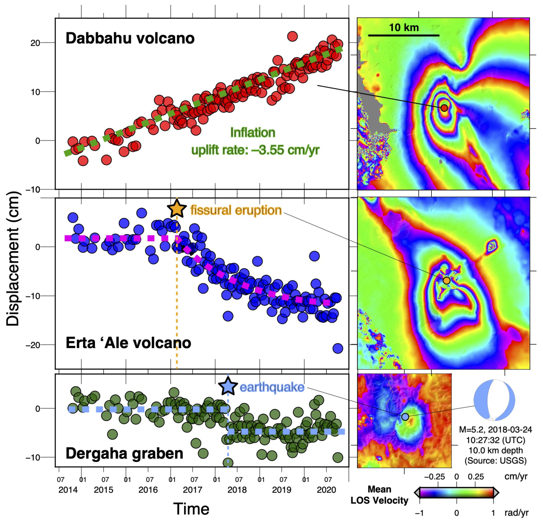
  • Following a major rifting episode that took place between 2005 and 2011 [55], the Dabbahu volcano (located North West of Manda Hararo in Figure 18) has experienced a steady re-inflation, inducing uplift at a rate of ≈3.5 cm/yr. The inflation is remarkably constant between 2014 and 2021, confirming the findings of [56];
  • In contrast, the volcano Erta ’Ale has shown a transient deflation that started in January 2017 following a lava lake overflow event, that produced long-lived lava flows [57];
  • Finally, a very small signal is detected in the Dergaha graben, coinciding with a cluster of seismicity detected in 2008 [58]. The time-series shows a clear step around March 2018, which corresponds well with the time of occurrence of the largest event of the seismic sequence.
Note that no low-pass filtering nor model adjustment have been applied on the time series presented here. They can therefore be safely interpreted, and uncertainties on the geophysical interpretation can be assessed using the dispersion of the time series.

6. Conclusions and Future Work

The FLATSIM service is dedicated to the monitoring of surface deformation of broad areas (i.e., larger than 250,000 km2). It aims at providing accurate measurements of ground displacements for a large range of geophysical applications, as pointed out in Section 5.2 and Section 5.3, mostly in natural environments. The service is a collaborative effort between InSAR experts, researchers in geophysics, and CNES engineers. Scientists provide their expertise on multi-temporal InSAR processing with a state of the art processing chain (NSBAS v2.0) and on geophysical processes, while CNES supports the implementation and deployment of this service in an operational mode. Taking advantage of the CNES mirroring of the Sentinel-1 data, as part of the PEPS infrastructure, this service benefits from rapid access to large volumes of imagery, a prerequisite for the efficient execution of the processing chain. The success of the implementation relies (1) on the algorithm of the NSBAS stack processing, with a single reference image for the whole image stack, avoiding redundant copies of input data, together with optimizations for a large number of steps, but more importantly, (2) on the specific, parallel NSBAS chain implementation on the CNES HPC infrastructure, with local transfer of input–output data on cluster nodes, allowing very fast I/O between disk and processors.
Since the goal of the service is to serve scientific purposes, the processed regions are selected according to scientific criteria. FLATSIM thus provides a set of products (e.g., the DTs product) that allows the end-users that do not have large computational capabilities to take advantage of the MTInSAR methodology, making an optimal use of the wealth of data provided by the Sentinel-1 mission. Moreover, a set of auxiliary data is also provided, which allows for assessing the quality of the delivered products. The product versatility makes possible their direct use by the end-users: for example by using the velocity maps as provided, ingesting the time-series in signal detection algorithms (e.g., principal component analysis, independent component analysis, geophysical modeling, …), or even by reprocessing individual interferograms or reinverting the time-series. Since the products are given a DOI, they can be cited.
In the future, the NSBAS processing chain will continue to evolve to integrate the most recent advances in InSAR processing. As the FLATSIM service has entered its operational phase, the core processing chain is anticipated to be updated at most twice a year. Another step will consist in providing the user with visualization capabilities, either online or with stand-alone tools, that will allow to explore more deeply into the delivered products.

Author Contributions

Conceptualization, M.-P.D., and C.L. (Cécile Lasserre); Funding acquisition, E.D.-O., and C.P.; Project administration, C.P.; Software, F.T., D.C., M.-P.D., C.L. (Christophe Laurent), E.P. (Erwan Pathier), E.P. (Elisabeth Pointal), and B.S.; Supervision, F.T., M.-P.D., and J.D.; Validation, M.-P.D., P.D., R.G., and C.L. (Cécile Lasserre); Writing—original draft, F.T., D.C., M.-P.D., J.D., P.D., R.G., C.L. (Christophe Laurent), C.L. (Cécile Lasserre), E.D.-O., E.P. (Erwan Pathier), E.P. (Elisabeth Pointal), C.P., and B.S.; Writing—review and editing, F.T., and M.-P.D. Except for the first author, who has supervised the writing of the paper, authors have been listed by alphabetical order. All authors have read and agreed to the published version of the manuscript.

Funding

This research was funded by CNES and ForM@Ter (internal funding).

Acknowledgments

The development, automation and optimization of the NSBAS chain necessary for this work was supported by CNES, focused on Sentinel-1 mission, under the project “DAT-S1: Déformation actuelle au Tibet mesurée par Sentinel-1”. Copernicus Sentinel data 2014–2020, processed by ESA, were retrieved from CNES PEPS platform. We wish to thank Michel Diament who supported this work on behalf of the ForM@Ter structure. We thank two anonymous reviewers for their helpful comments.

Conflicts of Interest

The authors declare no conflict of interest.

References

  1. Gabriel, A.; Goldstein, R.M.; Zebker, H. Mapping small elevation changes over large areas: Differential radar interferometry. J. Geophys. Res. 1989, 94, 9183–9191. [Google Scholar] [CrossRef]
  2. Massonnet, D.; Rossi, M.; Carmona, C.; Adragna, F.; Peltzer, G.; Feigl, K.; Rabaute, T. The displacement field of the Landers earthquake mapped by radar interferometry. Nature 1993, 364, 138–142. [Google Scholar] [CrossRef]
  3. Peltzer, G.; Rosen, P. Surface Displacements of the 17 May 1993 Eureka Valley, California, Earthquake Observed by SAR Interferometry. Science 1995, 268, 1333–1336. [Google Scholar] [CrossRef]
  4. Berardino, P.; Fornaro, G.; Lanari, R.; Sansosti, E. A new algorithm for surface deformation monitoring based on small baseline differential SAR interferograms. IEEE Trans. Geosci. Remote Sens. 2002, 40, 2375–2383. [Google Scholar] [CrossRef] [Green Version]
  5. Ferretti, A.; Prati, C.; Rocca, F. Permanent Scatterers in SAR Interferometry. IEEE Trans. Geosci. Remote Sens. 2001, 39, 8–20. [Google Scholar] [CrossRef]
  6. Schmidt, D.A.; Bürgmann, R. Time-dependent land uplift and subsidence in the Santa Clara valley, California, from a large interferometric synthetic aperture radar data set. J. Geophys. Res. 2003, 108. [Google Scholar] [CrossRef] [Green Version]
  7. Ferretti, A.; Fumagalli, A.; Novali, F.; Prati, C.; Rocca, F.; Rucci, A. A new algorithm for processing interferometric data-stacks: SqueeSAR. IEEE Trans. Geosci. Remote Sens. 2011, 49, 3460–3470. [Google Scholar] [CrossRef]
  8. Peltzer, G.; Crampé, F.; Hensley, S.; Rosen, P. Transient strain accumulation and fault interaction in the Eastern California shear zone. Geology 2001, 29, 975–978. [Google Scholar] [CrossRef]
  9. Wright, T.; Parsons, B.; Fielding, E. Measurement of interseismic strain accumulation across the North Anatolian Fault by satellite radar interferometry. Geophys. Res. Lett. 2001, 28, 2117–2120. [Google Scholar] [CrossRef]
  10. Doubre, C.; Peltzer, G. Fluid-controlled faulting process in the Asal Rift, Djibouti, from 8-year radar interferometry observations. Geology 2007, 35, 69–72. [Google Scholar] [CrossRef]
  11. Jolivet, R.; Lasserre, C.; Doin, M.P.; Peltzer, G.; Avouac, J.P.; Sun, J.; Dailu, R. Spatio-temporal evolution of aseismic slip along the Haiyuan fault, China: Implications for fault frictional properties. Earth Planet. Sci. Lett. 2013, 377–378, 23–33. [Google Scholar] [CrossRef]
  12. Bacques, G.; de Michele, M.; Raucoules, D.; Aochi, H.; Rolandone, F. Shallow deformation of the San Andreas fault 5 years following the 2004 Parkfield earthquake (Mw6) combining ERS2 and Envisat InSAR. Sci. Rep. 2018, 8, 6032. [Google Scholar] [CrossRef]
  13. Aslan, G.; Lasserre, C.; Cakir, Z.; Ergintav, S.; Ozarpaci, S.; Dogan, U.; Bilham, R.; Renard, F. Shallow Creep Along the 1999 Izmit Earthquake Rupture (Turkey) From GPS and High Temporal Resolution Interferometric Synthetic Aperture Radar Data (2011-2017). J. Geophys. Res. Solid Earth 2019, 124, 2218–2236. [Google Scholar] [CrossRef]
  14. Maubant, L.; Pathier, E.; Daout, S.; Radiguet, M.; Doin, M.P.; Kazachkina, E.; Kostoglodov, V.; Cotte, N.; Walpersdorf, A. Independent Component Analysis and Parametric Approach for Source Separation in InSAR Time Series at Regional Scale: Application to the 2017–2018 Slow Slip Event in Guerrero (Mexico). J. Geophys. Res. Solid Earth 2020, 125. [Google Scholar] [CrossRef]
  15. Daout, S.; Doin, M.P.; Peltzer, G.; Socquet, A.; Lasserre, C. Large-scale InSAR monitoring of permafrost freeze-thaw cycles on the Tibetan Plateau. Geophys. Res. Lett. 2017, 44, 901–909. [Google Scholar] [CrossRef]
  16. Solaro, G.; Acocella, V.; Pepe, S.; Ruch, J.; Neri, M.; Sansosti, E. Anatomy of an unstable volcano from InSAR: Multiple processes affecting flank instability at Mt. Etna, 1994–2008. J. Geophys. Res. Solid Earth 2010, 115. [Google Scholar] [CrossRef]
  17. Chen, Y.; Remy, D.; Froger, J.L.; Peltier, A.; Villeneuve, N.; Darrozes, J.; Perfettini, H.; Bonvalot, S. Long-term ground displacement observations using InSAR and GNSS at Piton de la Fournaise volcano between 2009 and 2014. Remote Sens. Environ. 2017, 194, 230–247. [Google Scholar] [CrossRef]
  18. Cavalié, O.; Doin, M.P.; Lasserre, C.; Briole, P. Ground motion measurement in the Lake Mead area, Nevada, by differential synthetic aperture radar interferometry time series analysis: Probing the lithosphere rheological structure. J. Geophys. Res. Solid Earth 2007, 112. [Google Scholar] [CrossRef] [Green Version]
  19. Doin, M.P.; Twardzik, C.; Ducret, G.; Lasserre, C.; Guillaso, S.; Jianbao, S. InSAR measurement of the deformation around Siling Co Lake: Inferences on the lower crust viscosity in central Tibet. J. Geophys. Res. Solid Earth 2015, 120, 5290–5310. [Google Scholar] [CrossRef]
  20. Pousse Beltran, L.; Pathier, E.; Jouanne, F.; Vassallo, R.; Reinoza, C.; Audemard, F.; Doin, M.P.; Volat, M. Spatial and temporal variations in creep rate along the El Pilar fault at the Caribbean-South American plate boundary (Venezuela), from InSAR. J. Geophys. Res. Solid Earth 2016, 121, 8276–8296. [Google Scholar] [CrossRef]
  21. Wang, H.; Wright, T.J. Satellite geodetic imaging reveals internal deformation of western Tibet. Geophys. Res. Lett. 2012, 39. [Google Scholar] [CrossRef] [Green Version]
  22. Daout, S.; Doin, M.P.; Peltzer, G.; Lasserre, C.; Socquet, A.; Volat, M.; Sudhaus, H. Strain Partitioning and Present-Day Fault Kinematics in NW Tibet From Envisat SAR Interferometry. J. Geophys. Res. Solid Earth 2018, 123, 2462–2483. [Google Scholar] [CrossRef]
  23. Weiss, J.R.; Walters, R.J.; Morishita, Y.; Wright, T.J.; Lazecky, M.; Wang, H.; Hussain, E.; Hooper, A.J.; Elliott, J.R.; Rollins, C. High-Resolution Surface Velocities and Strain for Anatolia From Sentinel-1 InSAR and GNSS Data. Geophys. Res. Lett. 2020, 47, 87376. [Google Scholar] [CrossRef]
  24. De Zan, F.; Monti Guarnieri, A. TOPSAR: Terrain Observation by Progressive Scans. IEEE Trans. Geosci. Remote Sens. 2006, 44, 2352–2360. [Google Scholar] [CrossRef]
  25. SNAP-ESA Sentinel Application Platform v2.0.2. Available online: http://step.esa.int (accessed on 10 September 2021).
  26. Rosen, P.A.; Gurrola, E.; Sacco, G.F.; Zebker, H. The InSAR scientific computing environment. In Proceedings of the EUSAR 2012 9th European Conference on Synthetic Aperture Radar, Nuremberg, Germany, 23–26 April 2012; pp. 730–733. [Google Scholar]
  27. Sandwell, D.; Mellors, R.; Tong, X.; Wei, M.; Wessel, P. Open radar interferometry software for mapping surface Deformation. EOS Trans. Am. Geophys. Union 2011, 92, 234. [Google Scholar] [CrossRef] [Green Version]
  28. Wegnüller, U.; Werner, C.; Strozzi, T.; Wiesmann, A.; Frey, O.; Santoro, M. Sentinel-1 Support in the GAMMA Software. Procedia Comput. Sci. 2016, 100, 1305–1312. [Google Scholar] [CrossRef] [Green Version]
  29. De Luca, C.; Cuccu, R.; Elefante, S.; Zinno, I.; Manunta, M.; Casola, V.; Rivolta, G.; Lanari, R.; Casu, F. An On-Demand Web Tool for the Unsupervised Retrieval of Earth’s Surface Deformation from SAR Data: The P-SBAS Service within the ESA G-POD Environment. Remote Sens. 2015, 7, 15630–15650. [Google Scholar] [CrossRef] [Green Version]
  30. Cigna, F.; Tapete, D. Sentinel-1 Big Data Processing with P-SBAS InSAR in the Geohazards Exploitation Platform: An Experiment on Coastal Land Subsidence and Landslides in Italy. Remote Sens. 2021, 13, 885. [Google Scholar] [CrossRef]
  31. Ferretti, A.; Novali, F.; Giannico, C.; Uttini, A.; Iannicella, I.; Mizuno, T. A Squeesar Database Over the Entire Japanese Territory. In Proceedings of the IGARSS 2019 IEEE International Geoscience and Remote Sensing Symposium, Yokohama, Japan, 28 July–2 August 2019; pp. 2078–2080. [Google Scholar] [CrossRef]
  32. Bischoff, C.A.; Ferretti, A.; Novali, F.; Uttini, A.; Giannico, C.; Meloni, F. Nationwide deformation monitoring with SqueeSAR® using Sentinel-1 data. Int. Assoc. Hydrol. Sci. 2020, 382, 31–37. [Google Scholar] [CrossRef] [Green Version]
  33. Kalia, A.; Frei, M.; Lege, T. A Copernicus downstream-service for the nationwide monitoring of surface displacements in Germany. Remote Sens. Environ. 2017, 202, 234–249. [Google Scholar] [CrossRef]
  34. Dehls, J.F.; Larsen, Y.; Marinkovic, P.; Lauknes, T.R.; Stødle, D.; Moldestad, D.A. A National Insar Deformation Mapping/Monitoring Service In Norway—From Concept To Operations. In Proceedings of the IGARSS, 2019 IEEE International Geoscience and Remote Sensing Symposium, Yokohama, Japan, 28 July–2 August 2019; pp. 5461–5464. [Google Scholar] [CrossRef]
  35. Papoutsis, I.; Kontoes, C.; Alatza, S.; Apostolakis, A.; Loupasakis, C. InSAR Greece with Parallelized Persistent Scatterer Interferometry: A National Ground Motion Service for Big Copernicus Sentinel-1 Data. Remote Sens. 2020, 12, 3207. [Google Scholar] [CrossRef]
  36. Bekaert, D.; Karim, M.; Linick, J.P.; Hua, H.; Sangha, S.; Lucas, M.; Malarout, N.; Agram, P.; Pan, L.; Owen, S. Development of open-access Standardized InSAR Displacement Products by the Advanced Rapid Imaging and Analysis (ARIA) Project for Natural Hazards. In Proceedings of the AGU Fall Meeting 2019, San Francisco, CA, USA, 9–13 December 2019. [Google Scholar]
  37. Lazecký, M.; Spaans, K.; González, P.J.; Maghsoudi, Y.; Morishita, Y.; Albino, F.; Elliott, J.; Greenall, N.; Hatton, E.; Hooper, A. LiCSAR: An Automatic InSAR Tool for Measuring and Monitoring Tectonic and Volcanic Activity. Remote Sens. 2020, 12, 2430. [Google Scholar] [CrossRef]
  38. Morishita, Y.; Lazecky, M.; Wright, T.; Weiss, J.; Elliott, J.; Hooper, A. LiCSBAS: An Open-Source InSAR Time Series Analysis Package Integrated with the LiCSAR Automated Sentinel-1 InSAR Processor. Remote Sens. 2020, 12, 424. [Google Scholar] [CrossRef] [Green Version]
  39. Doin, M.; Guillaso, S.; Jolivet, R.; Lasserre, C.; Ducret, G.; Grandin, R.; Pathier, E.; Pinel, V. Presentation of the small baseline NSBAS processing chain on a case example: The Etna deformation monitoring from 2003 to 2010 using Envisat data. In Proceedings of the Fringe 2011 Workshop, Frascati, Italy, 19–23 September 2011. [Google Scholar]
  40. Grandin, R. Interferometric processing of SLC Sentinel-1 TOPS data. In Proceedings of the FRINGE’15, Advances in the Science and Applications of SAR Interferometry and Sentinel-1 InSAR Workshop, Frascati, Italy, 23–27 March 2015. [Google Scholar]
  41. Rosen, P.A.; Hensley, S.; Peltzer, G.; Simons, M. Updated repeat orbit interferometry package released. EOS Trans. Am. Geophys. Union 2004, 85, 47. [Google Scholar] [CrossRef]
  42. Minh, D.H.T.; Doin, M.P.; Pathier, E.; Hanssen, R. Advanced methods in time series InSAR. In Displacement Measurement by Remote Sensing Imagery; Wiley: Hoboken, NJ, USA, 2021. [Google Scholar]
  43. Grandin, R.; Klein, E.; Métois, M.; Vigny, C. Three-dimensional displacement field of the 2015 Mw8. 3 Illapel earthquake (Chile) from across-and along-track Sentinel-1 TOPS interferometry. Geophys. Res. Lett. 2016, 43, 2552–2561. [Google Scholar] [CrossRef] [Green Version]
  44. Farr, T.G.; Rosen, P.A.; Caro, E.; Crippen, R.; Duren, R.; Hensley, S.; Kobrick, M.; Paller, M.; Rodriguez, E.; Roth, L. The Shuttle Radar Topography Mission. Rev. Geophys. 2007, 45. [Google Scholar] [CrossRef] [Green Version]
  45. Ansari, H.; De Zan, F.; Parizzi, A. Study of Systematic Bias in Measuring Surface Deformation with SAR Interferometry. IEEE Trans. Geosci. Remote Sens. 2021, 59, 1285–1301. [Google Scholar] [CrossRef]
  46. Prats-Iraola, P.; Scheiber, R.; Marotti, L.; Wollstadt, S.; Reigber, A. TOPS Interferometry With TerraSAR-X. IEEE Trans. Geosci. Remote Sens. 2012, 50, 3179–3188. [Google Scholar] [CrossRef] [Green Version]
  47. Pinel-Puyssegur, B.; Michel, R.; Avouac, J.P. Multi-Link InSAR Time Series: Enhancement of a Wrapped Interferometric Database. IEEE J. Sel. Top. Appl. Earth Obs. Remote Sens. 2012, 5, 784–794. [Google Scholar] [CrossRef]
  48. Doin, M.P.; Lasserre, C.; Peltzer, G.; Cavalié, O.; Doubre, C. Corrections of stratified tropospheric delays in SAR interferometry: Validation with global atmospheric models. J. Appl. Geophys. 2009, 69, 35–50. [Google Scholar] [CrossRef]
  49. Jolivet, R.; Grandin, R.; Lasserre, C.; Doin, M.P.; Peltzer, G. Systematic InSAR tropospheric phase delay corrections from global meteorological reanalysis data. Geophys. Res. Lett. 2011, 38. [Google Scholar] [CrossRef] [Green Version]
  50. Hersbach, H.; Bell, B.; Berrisford, P.; Hirahara, S.; Horányi, A.; Muñoz-Sabater, J.; Nicolas, J.; Peubey, C.; Radu, R.; Schepers, D. The ERA5 global reanalysis. Q. J. R. Meteorol. Soc. 2020, 146, 1999–2049. [Google Scholar] [CrossRef]
  51. Grandin, R.; Doin, M.P.; Bollinger, L.; Pinel-Puysségur, B.; Ducret, G.; Jolivet, R.; Sapkota, S.N. Long-term growth of the Himalaya inferred from interseismic InSAR measurement. Geology 2012, 40, 1059–1062. [Google Scholar] [CrossRef] [Green Version]
  52. López-Quiroz, P.; Doin, M.P.; Tupin, F.; Briole, P.; Nicolas, J.M. Time series analysis of Mexico City subsidence constrained by radar interferometry. J. Appl. Geophys. 2009, 69, 1–15. [Google Scholar] [CrossRef]
  53. Ryder, I.; Bürgmann, R.; Pollitz, F. Lower crustal relaxation beneath the Tibetan Plateau and Qaidam Basin following the 2001 Kokoxili earthquake. Geophys. J. Int. 2011, 187, 613–630. [Google Scholar] [CrossRef] [Green Version]
  54. Liu, S.; Xu, X.; Klinger, Y.; Nocquet, J.M.; Chen, G.; Yu, G.; Jónsson, S. Lower Crustal Heterogeneity Beneath the Northern Tibetan Plateau Constrained by GPS Measurements Following the 2001 Mw7.8 Kokoxili Earthquake. J. Geophys. Res. Solid Earth 2019, 124, 11992–12022. [Google Scholar] [CrossRef] [Green Version]
  55. Grandin, R.; Socquet, A.; Jacques, E.; Mazzoni, N.; de Chabalier, J.B.; King, G. Sequence of rifting in Afar, Manda-Hararo rift, Ethiopia, 2005–2009: Time-space evolution and interactions between dikes from interferometric synthetic aperture radar and static stress change modeling. J. Geophys. Res. Solid Earth 2010, 115. [Google Scholar] [CrossRef] [Green Version]
  56. Albino, F.; Biggs, J. Magmatic Processes in the East African Rift System: Insights From a 2015–2020 Sentinel-1 InSAR Survey. Geochem. Geophys. Geosyst. 2021, 22. [Google Scholar] [CrossRef]
  57. Moore, C.; Wright, T.; Hooper, A.; Biggs, J. The 2017 Eruption of Erta’Ale Volcano, Ethiopia: Insights into the shallow axial plumbing system of an incipient Mid-Ocean Ridge. Geochem. Geophys. Geosyst. 2019, 20, 5727–5743. [Google Scholar] [CrossRef]
  58. La Rosa, A.; Keir, D.; Doubre, C.; Sani, F.; Corti, G.; Leroy, S.; Ayele, A.; Pagli, C. Lower crustal earthquakes in the March 2018 sequence along the Western Margin of Afar. Geochem. Geophys. Geosyst. 2021, 22. [Google Scholar] [CrossRef]
Figure 1. Distribution of bursts as a function of acquisition dates (x-axis) and latitude (y-axis). Empty circles represent bursts that have not been kept, whereas blue circles correspond to bursts that have been selected for processing. Pink circles are bursts that have not been selected, but belong to the beginning or the end of a partially selected SAFE product (standard product produced by ESA that typically includes 9 bursts per sub-swath).
Remotesensing 13 03734 g001
Figure 2. (a) perpendicular baseline versus time for the Sentinel-1 descending track D079 on the Afar region (red dot indicates the primary date); (b) coregistration network; (c) histogram showing the distribution of time interval between consecutive acquisitions; (d) small-baseline interferogram network; (e) histogram showing the distribution of temporal baselines between acquisitions used for the calculated interferograms.
Remotesensing 13 03734 g002
Figure 3. Network-inversion of spectral diversity (a) and overlap between sub-swath (b). Error bars correspond to the averaged network discrepancy per acquisition. These two figures are part of the delivered products.
Remotesensing 13 03734 g003
Figure 4. Example of a wrapped interferogram in 32 looks and in radar geometry, before (a) and after (c) correction by the prediction from ERA-5 atmospheric model (panel (b)). For the 250 km wide southern segment of track D135 at the border between the Tibetan plateau and the Sichuan basin. One color cycle = 2.6 cm of delay. First date: 8 June 2020; second date: 20 June 2020.
Remotesensing 13 03734 g004
Figure 5. Processing steps for each interferogram.
Remotesensing 13 03734 g005
Figure 6. Time-series processing. The time series inversion provides, from the input stack of interferograms, maps of cumulative displacement, together with quality indicators. The mean velocity, obtained by linear regression through the time series, is shown in a wrapped color scale.
Remotesensing 13 03734 g006
Figure 7. General architecture for production and delivery.
Remotesensing 13 03734 g007
Figure 8. Production module architecture and components.
Remotesensing 13 03734 g008
Figure 9. Delivery module for user access.
Remotesensing 13 03734 g009
Figure 10. Catalog access architecture.
Remotesensing 13 03734 g010
Figure 11. Map of the selected regions of interest.
Remotesensing 13 03734 g011
Figure 12. Sentinel-1 tracks footprint of (a) the Afar case study, (b) the Tibetan case study.
Remotesensing 13 03734 g012
Figure 13. LOS velocity maps provided by automated FLATSIM processing in eastern Tibet over 15 separated track segments.The color scale is in rad/yr, positive away from satellite. The color scale amplitude from minimum to maximum, of 2.8 rad/yr, corresponds 12.5 mm/yr. The maps are overlying each other, from north to south and from east to west, i.e., only the segment on the south-west corner is displayed in its entirety. A constant velocity is added to individual maps to enhance visual continuity across the segments.
Remotesensing 13 03734 g013
Figure 14. Examples of quality indicators merged for the two segments of track A070 in Tibet.
Remotesensing 13 03734 g014
Figure 15. Quality indicators for track A070 in Tibet: (a) percentage of unwrapped area for all interferograms; (b) RMS misclosure for all interferograms; (c) RMS misclosure per date. Black curves: northern section. Red curve: southern section.
Remotesensing 13 03734 g015
Figure 16. Proxy for temporal coherence, merged for all tracks that have been processed in eastern Tibet. (a) Global map. (b) Zoom on the rectangle shown in (a). (c) Associated optical image. The red arrow points toward a large geometrical field of stabilized sand dunes. The blue arrow shows how dirt roads increase the coherence in desert sand dunes.
Remotesensing 13 03734 g016
Figure 17. Mean velocity map for track D079 and D006 showing a number of geophysical signals.
Remotesensing 13 03734 g017
Figure 18. Zoom on three geophysical signals. Areas of interest are indicated by the black rectangles in Figure 17.
Remotesensing 13 03734 g018
Table 1. Products of the interferogram package.
File TypeDescription
APSInterferogram Atmospheric Phase Screen from Global Atmospheric Model
InW/InUWrapped/Unwrapped Differential Interferograms
InWFWrapped Differential Filtered Interferograms
CohSpatial coherence
Table 2. Main timeseries products.
File TypeDescription
DTsTime series of total LOS phase delay (data cube)
MV-LOSMean LOS Velocity
NetAuxiliary maps for the assessment of the time series quality
Stk-InList of the interferograms file names
Table 3. Main auxiliary products.
File TypeDescription
CosENULOS unit vector expressed in local reference frame
(East, North, Up components).
DEMElevation in meter in radar geometry. Comes in two resolutions.
LuTLookup Tables used to do the mapping between radar and ground geometry.
TCohBackscatter properties in 2 looks.
Publisher’s Note: MDPI stays neutral with regard to jurisdictional claims in published maps and institutional affiliations.

