InSAR Coherence Analysis for Wetlands in Alberta, Canada Using Time-Series Sentinel-1 Data

Abstract

Wetlands are valuable natural resources which provide numerous services to the environment. Many studies have demonstrated the potential of various types of remote sensing datasets and techniques for wetland mapping and change analysis. However, there are a relatively low number of studies that have investigated the application of the Interferometric Synthetic Aperture Radar (InSAR) coherence products for wetland studies, especially over large areas. Therefore, in this study, coherence products over the entire province of Alberta, Canada (~661,000 km²) were generated using the Sentinel-1 data acquired from 2017 to 2020. Then, these products along with large amount of wetland reference samples were employed to assess the separability of different wetland types and their trends over time. Overall, our analyses showed that coherence can be considered as an added value feature for wetland classification and monitoring. The Treed Bog and Shallow Open Water classes showed the highest and lowest coherence values, respectively. The Treed Wetland and Open Wetland classes were easily distinguishable. When analyzing the wetland subclasses, it was observed that the Treed Bog and Shallow Open Water classes can be easily discriminated from other subclasses. However, there were overlaps between the signatures of the other wetland subclasses, although there were still some dates where these classes were also distinguishable. The analysis of multi-temporal coherence products also showed that the coherence products generated in spring/fall (e.g., May and October) and summer (e.g., July) seasons had the highest and lowest coherence values, respectively. It was also observed that wetland classes preserved coherence during the leaf-off season (15 August–15 October) while they had relatively lower coherence during the leaf-on season (i.e., 15 May–15 August). Finally, several suggestions for future studies were provided.

1. Introduction

Wetlands are important ecosystems that provide valuable services to the environment and humans. Wetlands have many benefits, including providing important habitat to many plants and animals, maintaining water quality, controlling floods, providing food and recreational opportunities for humans, and acting as carbon sinks [1,2,3]. Although wetlands are considered as the “kidneys” of the environment because of these valuable services, they are currently threatened by excessive agricultural expansion, water extraction for agricultural and industrial purposes, climate change, thawing of permafrost, construction of reservoirs, and deforestation [3,4,5]. Thus, accurate information about the type and extent of different wetlands and their changes over time especially over large areas is crucial.

Although field observations provide very accurate in situ data for wetland monitoring, these techniques are impractical for large-scale wetland classification and regular wetland monitoring. This is because field observations for wetland monitoring over large areas are expensive, time-consuming, and labor-intensive. Additionally, most wetlands are located in inaccessible areas, making field surveys impossible or costly [3,6,7]. On the other hand, remote sensing technology has enabled us to map and monitor wetlands at larger scales and anywhere in the world [3,8]. Satellite remote sensing methods for wetland studies have been developing for the past few decades and have now reached the point where they can cost-effectively produce up-to-date and accurate wetland classifications at large spatial scales [9,10,11]. In this regard, Synthetic Aperture Radar (SAR) systems are great resources due to several advantages.

SAR systems acquire data independent of atmospheric conditions. Therefore, they are suitable for wetland mapping in areas where clouds are present and the weather is not good [2,12]. Moreover, SAR data are great resources for monitoring surface water and its changes over time [13,14]. SAR signals, especially L-band data, can also penetrate through the vegetation canopy and allow the identification of flooded vegetation (e.g., emergent marsh), mainly due to the double-bounce scattering mechanism between water and emergent vegetation [15,16,17,18].

As mentioned earlier, SAR systems provide valuable data for spatio-temporal wetland change analysis. In this regard, the Interferometric SAR (InSAR) technique, which can be effectively employed for change detection purposes, provides valuable measurements for monitoring a variety of phenomena, such as water level fluctuations and wetland conditions [19,20,21]. Both the phase and amplitude of the received echoes are used to create InSAR products. These InSAR products consist of two radar images with varying temporal and spatial baselines. The interferometric phase ($\phi$) and coherence magnitude ($\gamma$) are the two InSAR observables for change detection applications [22,23,24]. $\gamma$ values range from zero to one and are affected by changes in surface properties, especially electrical properties [24,25]. Higher values indicate better interferogram quality, indicating no/low changes in the surface properties, such as vegetation cover and soil moisture. Changes in the ground characteristics reduce $\gamma$ values, which can be conceptually divided into temporal, spatial, and thermal decorrelation [26]. Thermal and spatial decorrelation refers to the system noise and the positions of the SAR sensor during the data acquisition, respectively. Temporal decorrelation refers to changes that occur between InSAR pairs, such as changes in surface properties (e.g., deformations, vegetation, soil moisture) or atmospheric conditions [26,27].

Recent studies have argued that SAR backscatter from flooded vegetation could lead to high coherence [14,15,17,28,29,30,31,32]. InSAR results also suggest that Coherence Change Detection (CCD) could be effectively used for monitoring wetlands [15]. $\gamma$ values may decrease over wetlands due to various decorrelation factors which can be associated with the characteristics of SAR systems (e.g., temporal and spatial baselines, and viewing angles) and wetland characteristics (e.g., vegetation density, growth, and types, water level, soil moisture, and phenology) [20]. Consequently, vegetation density, growth, and types, as well as water level fluctuations, soil moisture, and wetland classification can be mapped using InSAR. Recently, extensive analysis and reviews have been published on the applications of InSAR in wetlands [5,20,28,33]. For example, [34] used Small Temporal Baseline Subset (STBAS), a time series InSAR technique, to map wetland water levels in the Florida Everglades. The average RMSE of 6.6 cm was obtained when comparing the estimated and measured observations. They concluded that the uncertainties in the estimation were due to the accuracy of the InSAR technique and the ground data. Furthermore, [35] developed a new InSAR technique based on the distributed scatterer interferometry for detecting changes in wetland water depth in the Yellow River Delta from 2007 to 2010 using the Advanced Land Observation Satellite (ALOS) data. Their method adjusted an optimal interferogram network to obtain stability between reducing computational cost and preserving the maximum InSAR information. [15] also examined wetland vegetation characteristics that led to coherence in RADARSAT-2 InSAR data of an area in eastern Canada. The results demonstrated that most marshes and swamps maintained coherence throughout the ice- and snow-free period for the 24-day repeat cycle of RADARSAT-2. However, the coherence of open water was very noisy and could not be used for CCD and water level monitoring. Additionally, [20] discussed the advantages and limitations of InSAR techniques for wetland mapping and monitoring. They reviewed InSAR applications for hydraulic and hydrological analysis. In [36], C-band $\gamma$ time-series for wetland monitoring were also evaluated. The main result of their findings showed that $\gamma$ time-series could be used for monitoring land use impacts on wetland function. Finally, [37] investigated L-band InSAR observations ($\phi$ and $\gamma$) using ALOS/PALSAR for monitoring wetland water level and vegetation in different seasons between 2007 and 2011. The time-series of $\gamma$ showed seasonal variations with higher and lower coherence values during winter and summer, respectively. They also reported that $\gamma$ and the Normalized Difference Vegetation Index (NDVI) were inversely correlated.

Although recent studies have shown that InSAR coherence is a potential remote sensing product for wetland monitoring, it has not been fully investigated for province- or country-wide applications compared to other remote sensing datasets and techniques. Therefore, in this study, the potential of the coherence maps generated from Sentinel-1 data, acquired from 2017 to 2020 over the entire province of Alberta, Canada, were investigated for wetland mapping and change analysis. In this study, the first Alberta-wide temporal coherence maps (spring, summer and fall) were generated. Then, the results were investigated along with a large amount of wetland field data to assess the coherence variation for different wetland classes.

2. Material and Method

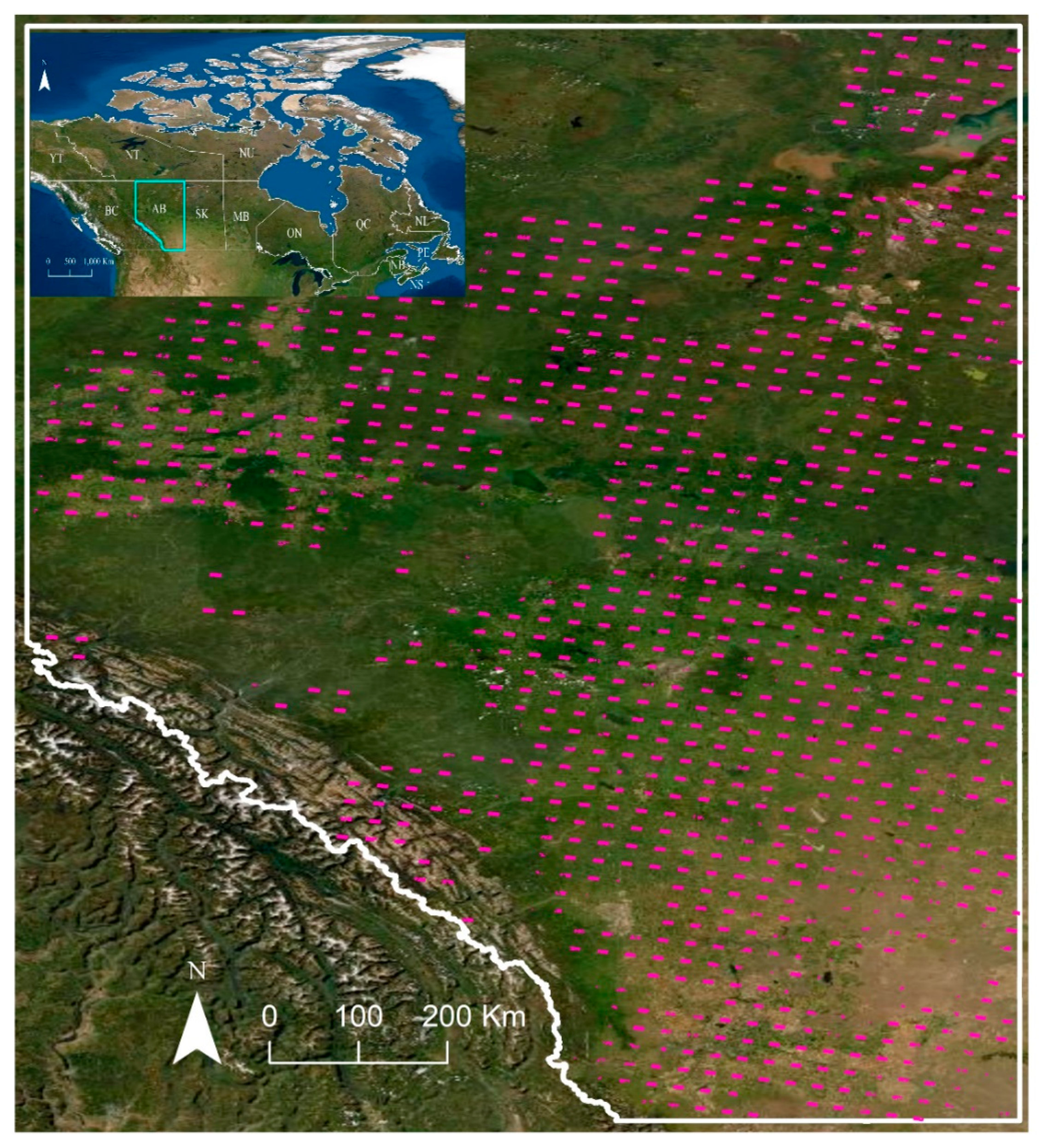
2.1. Study Area

The study area is the entire province of Alberta, with an area of 661,190 km² (latitude from 49°N to 60°N and longitude from 110°W to 114.07°W), located in the continental interior of western Canada (Figure 1). Alberta has a variety of land cover types and climate due to its large area [38]. In summer, daytime temperatures are usually around 20 to 25 °C but can reach up to 30 °C, and in winter (e.g., January and February), daytime temperatures range from −5 to −15 °C. The temperature can also drop as low as −40 °C for short periods.

The province is mainly covered by forests, wetlands, water bodies, pastures, agricultural lands, and urban areas. Wetlands are a prominent feature of the province and cover about 21% of the province [11,38]. All five wetland classes specified by the Canadian Wetland Classification System (CWCS; i.e., bog, fen, marsh, swamp, and shallow open water) are found in the province [38]. Although a large portion of the province is covered by wetlands, many have been disturbed by natural disasters, such as wildfires, anthropogenic activities (e.g., oil and gas explorations and agricultural and urban expansion) [7,38].

2.2. Reference Data

In this study, the grid of photo-interpretation plots (3 × 7 km² each), collected over the province of Alberta from 2010 to 2016 were used (Figure 1) [39]. Wetland types within each plot were classified by the Alberta Biodiversity Monitoring Institute (ABMI) using interpretation of 3D imagery at ~0.5 m spatial resolution. These reference samples were used to extract the coherence values of each wetland class. Figure 1 shows the distribution of the reference samples and

Table 1. Number (area/km²) of the reference polygons for the wetland classes.

	Treed Bog	Treed Fen	Open Fen	Open Marsh	Treed Swamp	Open Swamp	Shallow Open Water
# polygons (area)	2564 (298.05)	2925 (322.26)	12,970 (1455.48)	3421 (160.81)	12.035 (836.73)	2247 (191.44)	1993 (51.33)

provides the information on the number and area of samples (polygons) used in this study. As seen, seven wetland classes of Treed Bog, Fen (Treed and Open), Open Marsh, Swamp (Treed and Open), and Shallow Open Water (typically less than 2 m depth) were utilized in this study.

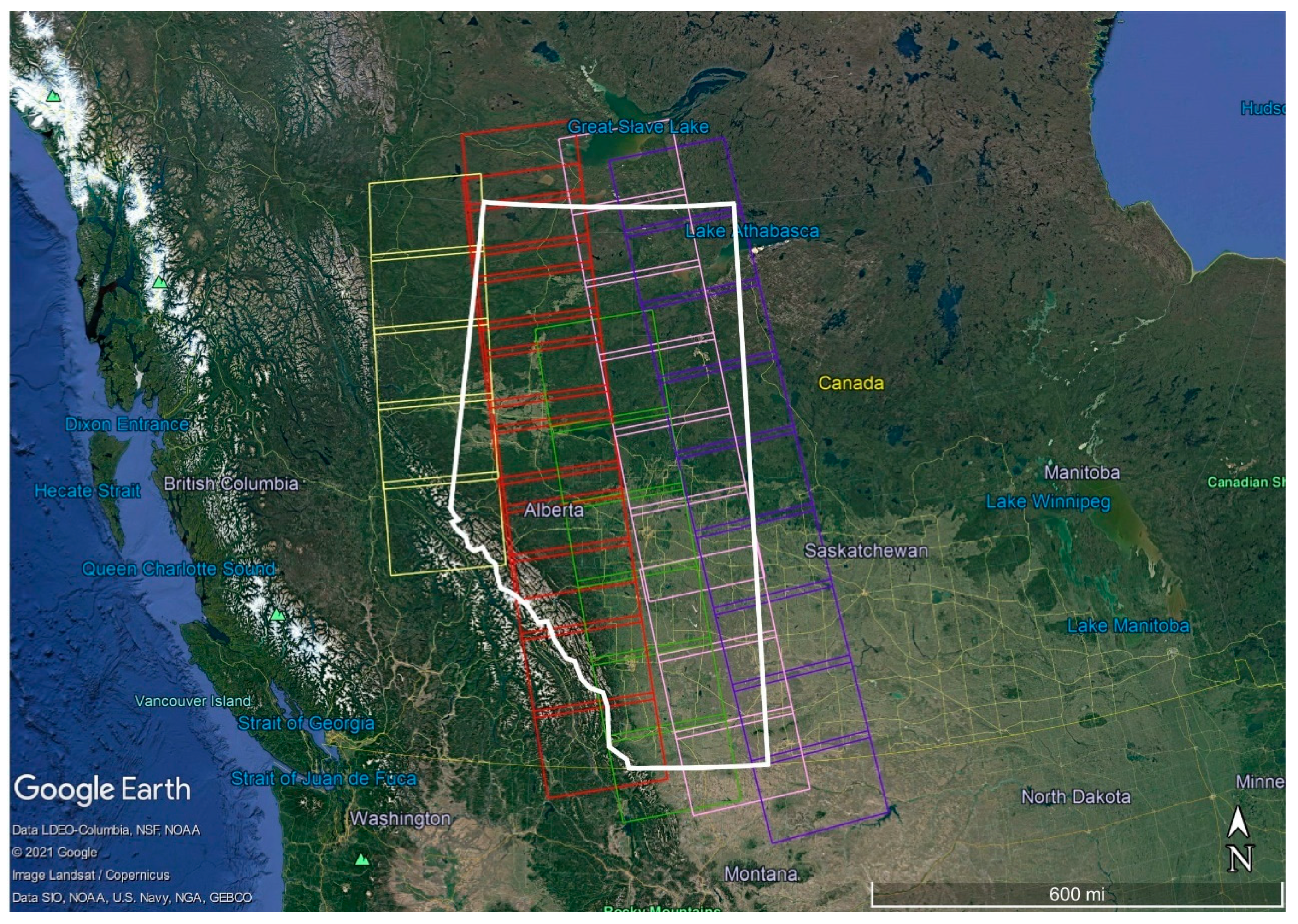
2.3. Satellite Data

The coherence products were generated from Sentinel-1 C-band SAR data. The temporal resolution of Sentinel-1 satellites is 6 days and can therefore be used effectively for frequent wetland mapping. Sentinel-1 C-band SAR data in five tracks of the satellites’ orbits (see Figure 2 for the footprints of the tracks over the study area), covering the entire province, were processed. These data were downloaded from National Aeronautics and Space Administration (NASA) Alaska Satellite Facility (ASF) archives [40] between May and October for the years 2017 to 2020. The Interferometric Wide (IW) swath mode in the VV polarization with a spatial resolution of 5 × 20 m (Single Look Complex (SLC) data) was utilized to generate the coherence products.

2.4. InSAR Processing and Coherence Values Extraction

Interferometry can provide coherence, which is a measure of the interferometric correlation between two co-registered SAR images. SLC SAR data is described by complex values (Equations (1) and (2)). For each SLC pixel, the phase difference between two SLCs (${\phi }_{m,n}$) can be calculated by multiplying reference image, $q_m$, with the complex conjugate (*) of secondary image, $q_n$ (Equation (3)) [41].

$$q_m=\left|q_m\right|\exp \left(j{\phi }_m\right)$$

(1)

$$q_n=\left|q_n\right|\exp \left(j{\phi }_n\right)$$

(2)

$$q_m·{q_n}^{*}=\left|q_m{q}_n\right|\exp \left[j({\phi }_m-{\phi }_n\right)]=\left|q_{m,n}\right|\exp \left({\phi }_{m,n}\right)$$

(3)

The amplitude of each pixel of the interferogram (|$q_{m,n}$|) is in proportion to the amplitudes of the two SLC images (|$q_m$|, (|$q_n$|)). Interferogram amplitudes significantly fluctuate even in the ideal cases of no spatio-temporal decorrelations. Therefore, the phase noise changes from one pixel to another due to the different effects of random noise superposed on the random amplitudes. Pixels with strong returns obtain reliable phases while unstable scatterers show more diffused interferometric phases. Additionally, there are considerable changes between the two SAR acquisitions due to the changes in the incidence angle and random noise. The measure of this change, which indicates the coherence (the complex correlation coefficient) of the two SLCs (${\gamma }_{m,n}$) is defined as follows [41]:

$${\gamma }_{m,n}=\frac{E\{q_m·{q_n}^{*}\}}{\sqrt{E\{{\left|q_m\right|}^2\}·E\{{\left|q_n\right|}^2\}}}=\left|{\gamma }_{m,n}\right|\exp \left(j{\phi }_{m,n}\right),\left|{\gamma }_{m,n}\right|<1$$

(4)

where InSAR coherence magnitude ($\left|{\gamma }_{m,n}\right|$) and InSAR phase (${\phi }_{m,n}$) are the magnitude and argument of the complex correlation coefficient, ${\gamma }_{n,m}$, between two acquisitions m and n, respectively [41]. ${\phi }_m$ and $\left|q_m\right|$ also respectively represent phase and SAR amplitude of the acquisition, $q_m$.

An interferogram created from two SAR scenes may be modelled as the sum of several phase components as described in Equation (5).

$${\phi }_{meas}={\phi }_{orbit}+{\phi }_{atm}+{\phi }_{topo}+{\phi }_{s{l}_{pos}}+{\phi }_{a{z}_{pos}}+{\phi }_{defo}+{\phi }_{noise}$$

(5)

where ${\phi }_{meas}, {\phi }_{orbit}, {\phi }_{atm}, {\phi }_{topo}, {\phi }_{s{l}_{pos}}, {\phi }_{defo}, {\phi }_{noise}$ are respectively the total measured phase difference between the reference and secondary SAR scenes, the residual phase resulting from inaccurate orbit information, the phase delay resulting from the atmospheric disturbances in both the reference and secondary scenes, the phase resulting from the imaged topography, phase related to the path length travelled within the resolution cell from the radar wavefront to the target along the slant-range direction, phase relating to the path length travelled within the resolution cell from the radar wavefront to the target along the azimuth direction, phase due to the displacement process, phase from the sum of the sensor’s thermal noise, decorrelation effects (changes in the backscattering pattern with time related to ground changes, vegetation development, and baseline and Doppler shift differences between the reference and secondary images and any other un-modelled factors).

Interferometric coherence is a measure of the phase uniformity between two SAR acquisitions. This means that any change in the phase components from Equation (5) will degrade the interferometric coherence. The influencing factors for each of the phase components are described below:

${\phi }_{orbit}$: this could lead to flat Earth phase fringes that could affect the coherence estimates. Through trial and error, the orbital parameters (e.g., perpendicular baseline and yaw angle) can be manually adjusted until the proper rate of flat Earth fringe is estimated and totally removed. The fringe rate estimation and removal can be also performed automatically using an adequate spatial filter and orbital modeling. For Sentinel-1, accurate orbits are available and orbit corrections are not required for the purpose of coherence estimation [42].

${\phi }_{atm}$: this remains an unsolved phase component. The tropospheric component of ${\phi }_{atm}$ could be considered to vary slowly in space and could be filtered out by a high-pass filter [43]. On the other hand, the water vapor content is highly variable spatially and it cannot be easily removed by spatial filtering [44]. It is complicated to estimate the exact characteristics of the atmospheric delay from the data and, therefore, residual atmospheric effects are likely to be present in the interferogram after filtering. It was reported that at the 3 × 3 or 5 × 5 pixels patch size used to estimate interferometric coherence, most of the atmospheric effects are constant and, thus, do not affect the coherence estimates [41].

${\phi }_{topo}$: this induces geometric decorrelation that could affect the coherence estimate. Sentinel-1 satellites were designed to be insensitive to topography by maintaining a very short perpendicular baseline [45] and, thus, steep topography leads to only a small topographic phase component. Additionally, a Digital Elevation Model (DEM) can be used to model and remove part of the topographic components. ${\phi }_{topo}$ could also include volumetric decorrelation due to steep vegetation [46].

${\phi }_{s{l}_{pos}},{\phi }_{a{z}_{pos}}$: these components cannot be estimated for extended targets. However, due to the small perpendicular baseline of Sentinel-1 and the very accurate ToPSAR co-registration in the azimuth direction (0.001 pixel RMSE), these components are negligible [47].

${\phi }_{defo}$: this could also affect the coherence estimation if the displacement process is very local (e.g., over an area of 3 × 3 pixels is approximately 36 × 10 m²). This is because phase variation due to displacement lowers the coherence estimates.

${\phi }_{noise}$: this is minimized by applying a spatial filter and maintaining the same temporal baseline (e.g., 12 days for Sentinel-1). The noise in interferometric phase is due to the changes in the scattering characteristics of targets between the two acquisitions, as well as thermal and processing noise. These mainly result in decorrelations. The amount of decorrelation is represented by the magnitude of the coherence (|${\gamma }_{m,n}$|). Different sources of decorrelation can be defined [26,41]. Temporal decorrelation can be caused by physical changes of the ground surface within the resolution cell. Geometric decorrelation, induced by different incidence angles of the radar signal [48], leads to a transition between the data frequency spectra of the images, resulting in noise. Furthermore, different Doppler centroid frequencies cause Doppler centroid decorrelation. Doppler decorrelation is the azimuthal equivalent of geometric decorrelation. Other sources of decorrelation include system and processing noises, which are caused by instrumental thermal noise and the processing of the SAR images, respectively. It should be noted that the very small perpendicular baseline of the Sentinel-1 satellites lowers the interferometric noise and maintain interferometric coherence [48].

In this study, the 12-day InSAR pairs were co-registered using the S1 TOPS co-registration method [49] to generate coherence products. The co-registration process was performed with a sub-pixel accuracy of 0.001 pixels RMSE. Then, $\left|\gamma \right|$, $\phi$ and SAR amplitudes were produced for all acquisitions. Finally, a filter was adaptively applied to the coherence products to reduce noise and increase coherence [46]. In this study, coherence was estimated from differential interferogram that can contain phase fringes at different rates, related to various factors, such as topography, ground dynamics, vegetation motion, and severe atmospheric events. Since coherence represents a measure of similarity (stability of interferometric phase), the presence of a fringe would be considered as a variable that degrades coherence. In order to avoid coherence degradation due to fringes, an adaptive filtering algorithm that matched the local fringe rate was used. By this, the dependence of coherence estimates to phase fringes was removed.

In total, 600 coherence products were generated from five Sentinel-1 tracks (see Figure 2) and mosaicked to cover all of Alberta and parts of Saskatchewan and British Columbia. After generating the coherence products, the reference polygons (see Section 2.2) were overlaid and the coherence values for each polygon were extracted. The average value of coherence within each polygon was considered as its coherence value. Finally, the coherence values of all polygons of each wetland class were averaged and considered as the final coherence value. These coherence values of different wetland classes were used to investigate their application in wetland classification and change analysis.

2.5. Scenarios for Wetland Coherence Assessment

Wetland types are different in terms of ecological, physical, and spectral characteristics. A single wetland type can be also divided into multiple subclasses due to different ecological characteristics. For instance, the Swamp class can be divided into treed and open swamps. Therefore, it is expected that coherence values are different for various wetland classes. Moreover, wetlands in Alberta are highly dynamic in time and, therefore, a wetland may look different at various times (e.g., years, seasons, and months). For example, vegetation density and water level in wetland areas are different in leaf-on/off seasons. Consequently, coherence values of wetlands can change at various times. In this study, all wetland classes were divided into four categories within three date scenarios to comprehensively investigate the coherence values of different wetland types at different times. The four categories are:

Category 1.

Wetland (i.e., Treed Bog, Treed Fen, Open Fen, Treed Swamp, Open Swamp, and Open Marsh).

Category 2.

Treed Wetland (i.e., Treed Bog, Treed Fen, and Treed Swamp) and Open Wetland (i.e., Open Fen, Open Marsh, and Open Swamp).

Category 3.

Treed Bog, Fen (i.e., Treed Fen and Open Fen), Open Marsh, Swamp (i.e., Treed Swamp and Open Swamp), and Shallow Open Water.

Category 4.

Treed Bog, Treed Fen, Open Fen, Open Marsh, Treed Swamp, and Shallow Open Water.

The three date scenarios are also:

Monthly: May, June, July, August, September, and October.

Seasonally: Spring (i.e., May), Summer (i.e., June, July, August), and Fall (September and October).

Leaf-on/off: Leaf-on (i.e., 15 May–15 August), Leaf-off (15 August–15 October). It should be noted that leaf-on/off dates are not consistent across all of Alberta and, therefore, the dates were chosen as the best approximation.

As is clear, the dates when snow or ice usually exist on the ground (i.e., 15 October to 15 May) were removed from the analyses. This was because snow and ice result in noisy coherence products.

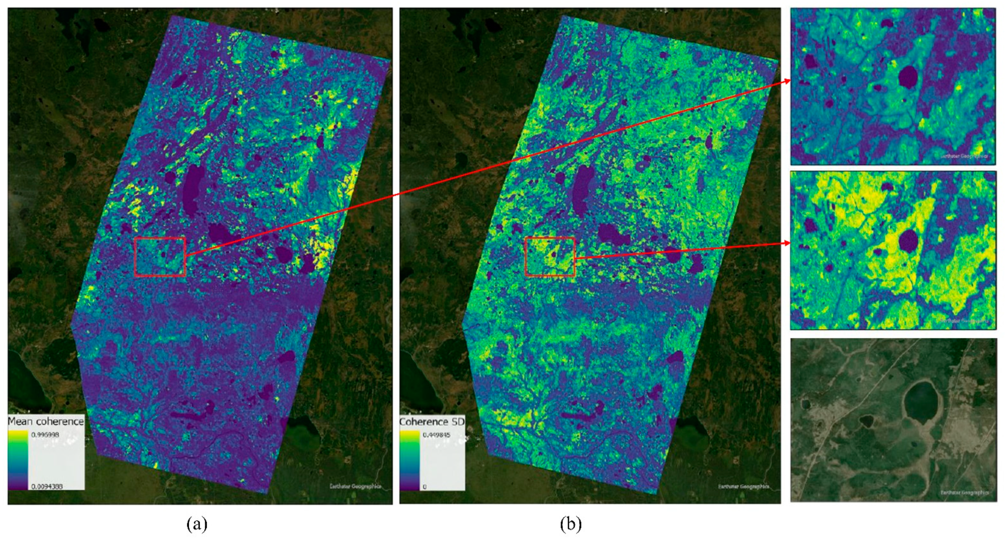
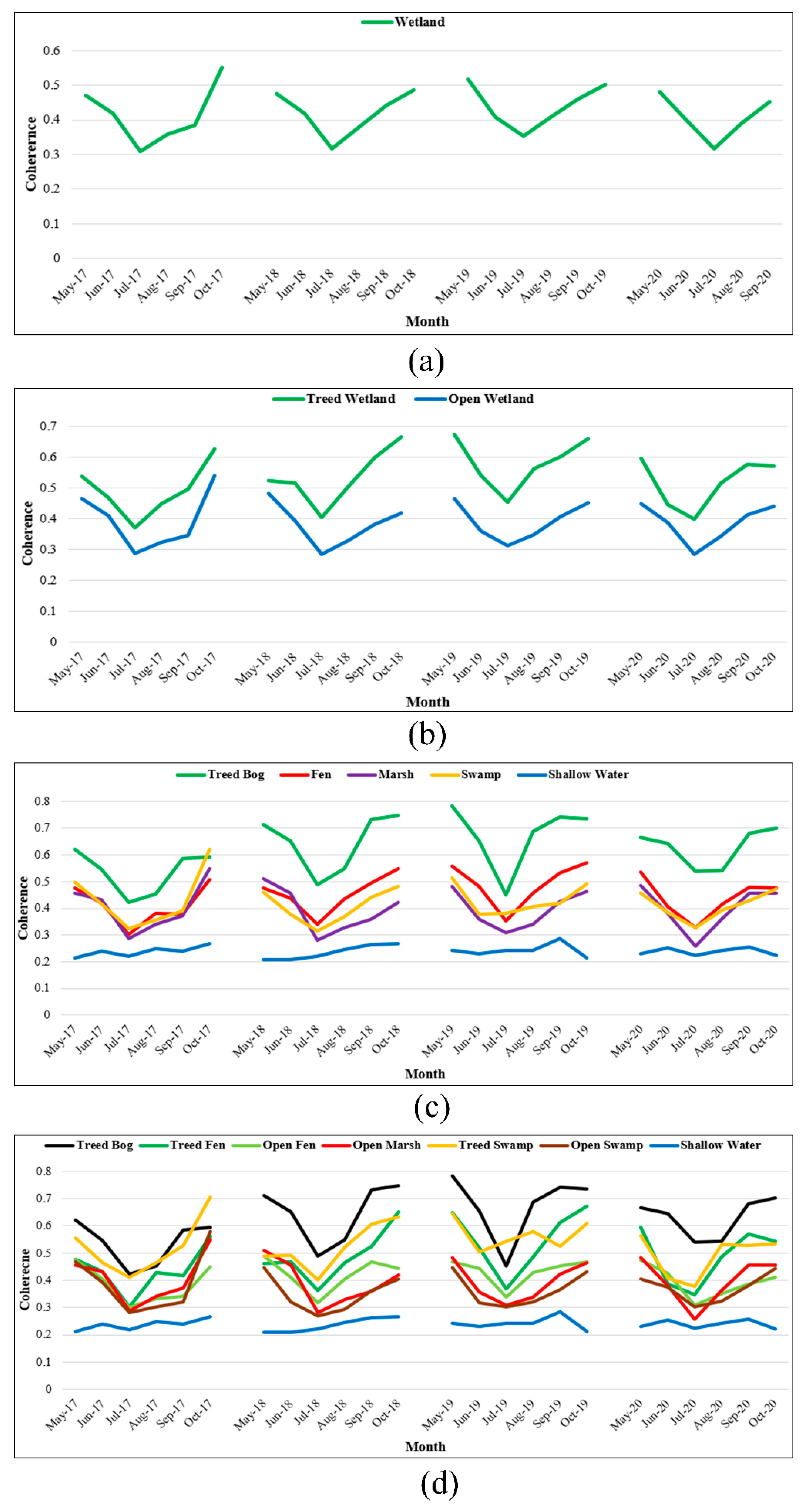
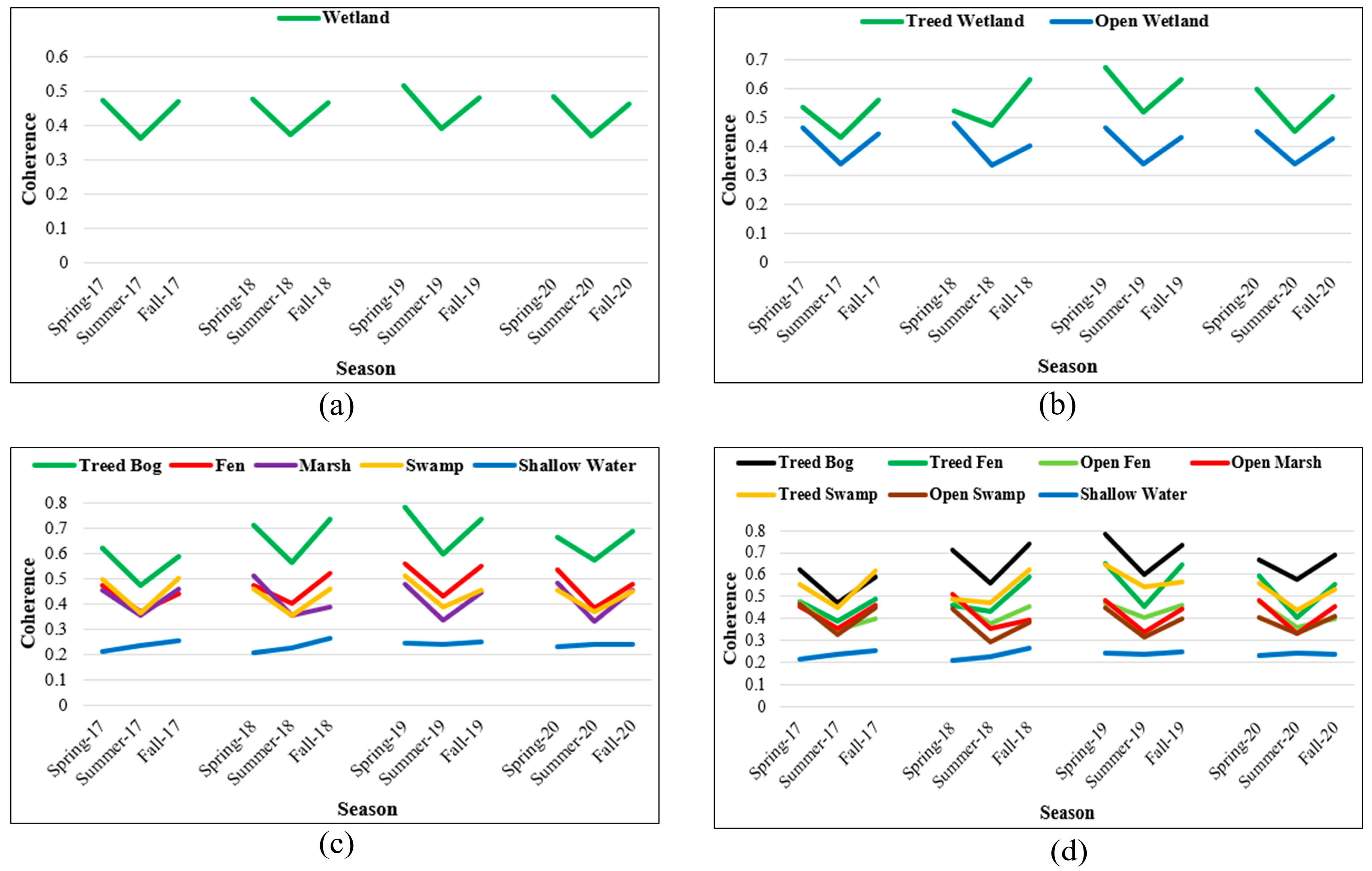
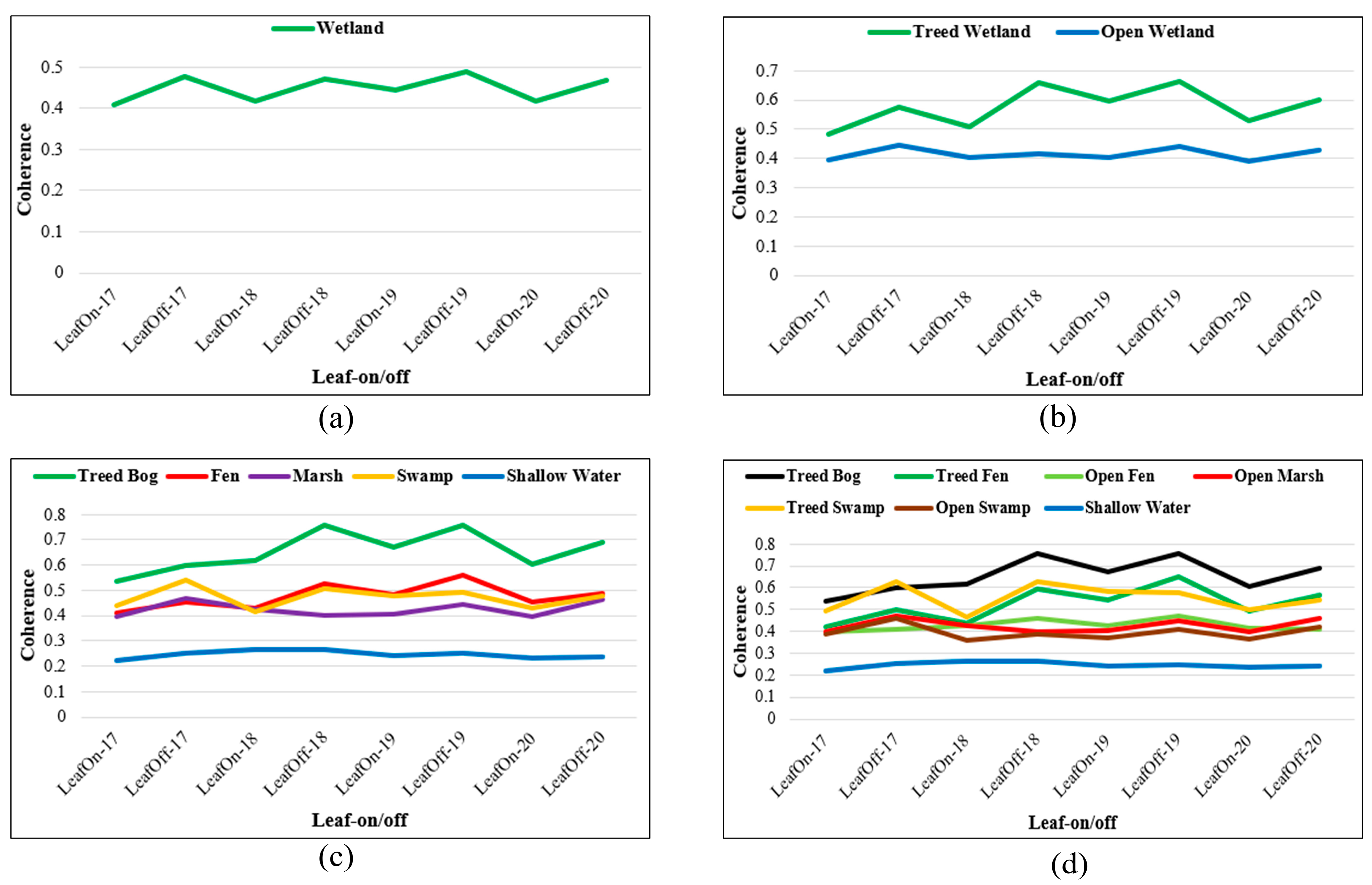
3. Results

Figure 3 illustrates one of the coherence maps in June 2020 from the entire province of Alberta. Several zoomed images of three wetland classes are also demonstrated to compare the coherence. As is clear from Figure 3, there are several artificial lines in the final Alberta-wide coherence map. This is because, the acquisition dates for adjacent tracks are different and, thus, coherence changes over different tracks. Different tracks in fact contain different coherence information and, therefore, there will be discontinuities when mosaicking coherence products from different dates (tracks) over the entire province. Practically, the coherence products from different track would be better to be analyzed separately.

The coherence values for treed wetlands were high, but those of the Shallow Open Water were very low. Overall, it was visually observed that coherence products were valuable products to discriminate different wetland classes. The time of the coherence product was the main factor which should be considered when using these products for wetland classification. For example, there were wetland classes which were not distinguishable using the summer products, but there were some opportunities to separate them using the coherence products generated in spring or summer. The temporal average and standard deviation of coherence maps for one of the tracks are also shown in Figure 4, illustrating high coherence values in treed wetlands as well as the lowest mean values in open water bodies. Areas with flooded vegetation could have high standard deviation of coherence (e.g., Figure 4b) if the flooding levels are varying or the vegetation on top suffers changes. Thus, high average and high standard deviation of coherence could indicate a fluctuating water levels under the vegetation or vegetation changes. To separate these two possible causes, several statistical analyses were performed on different time intervals, the results of which are provided in Section 3.1, Section 3.2 and Section 3.3.

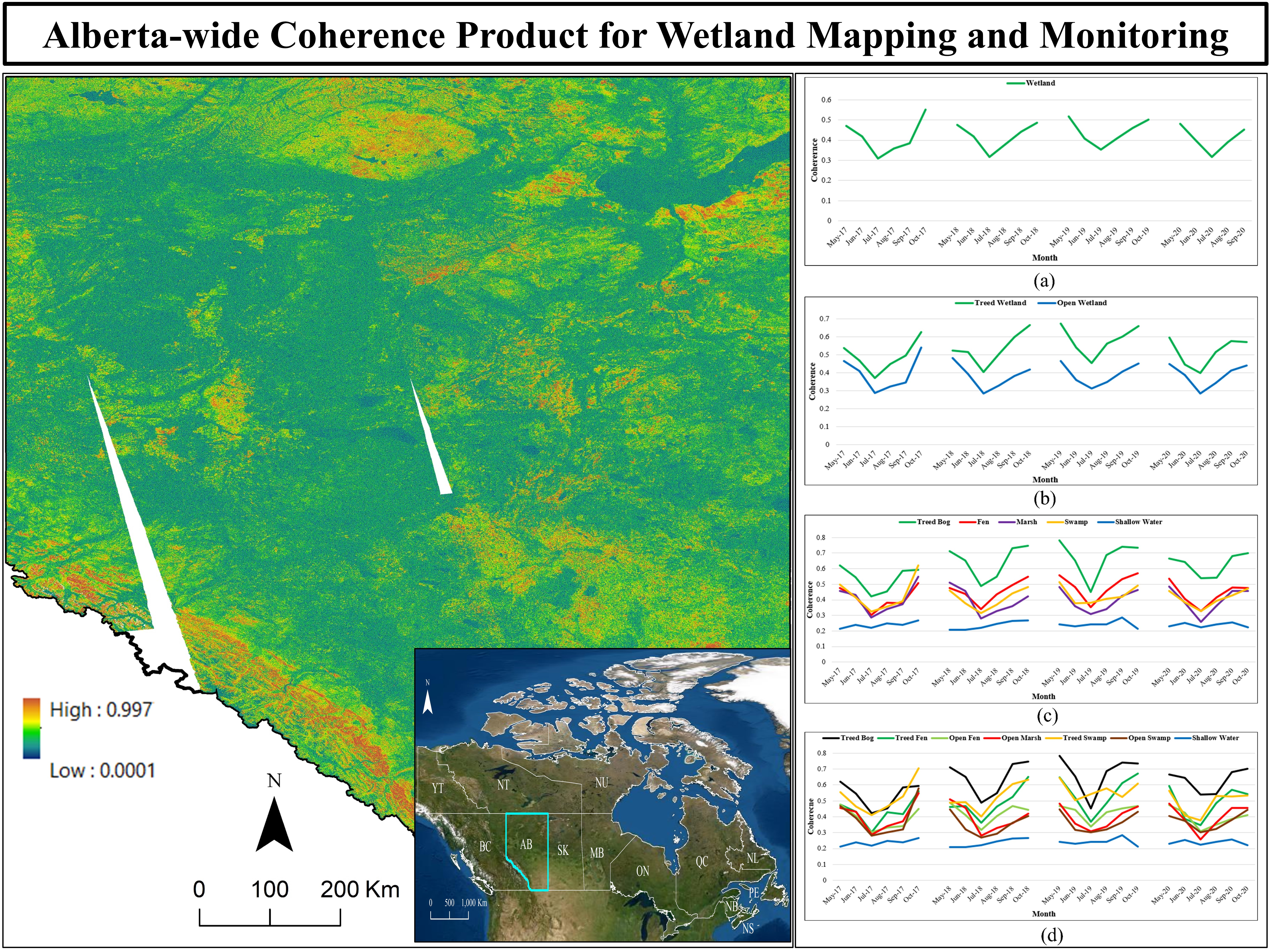
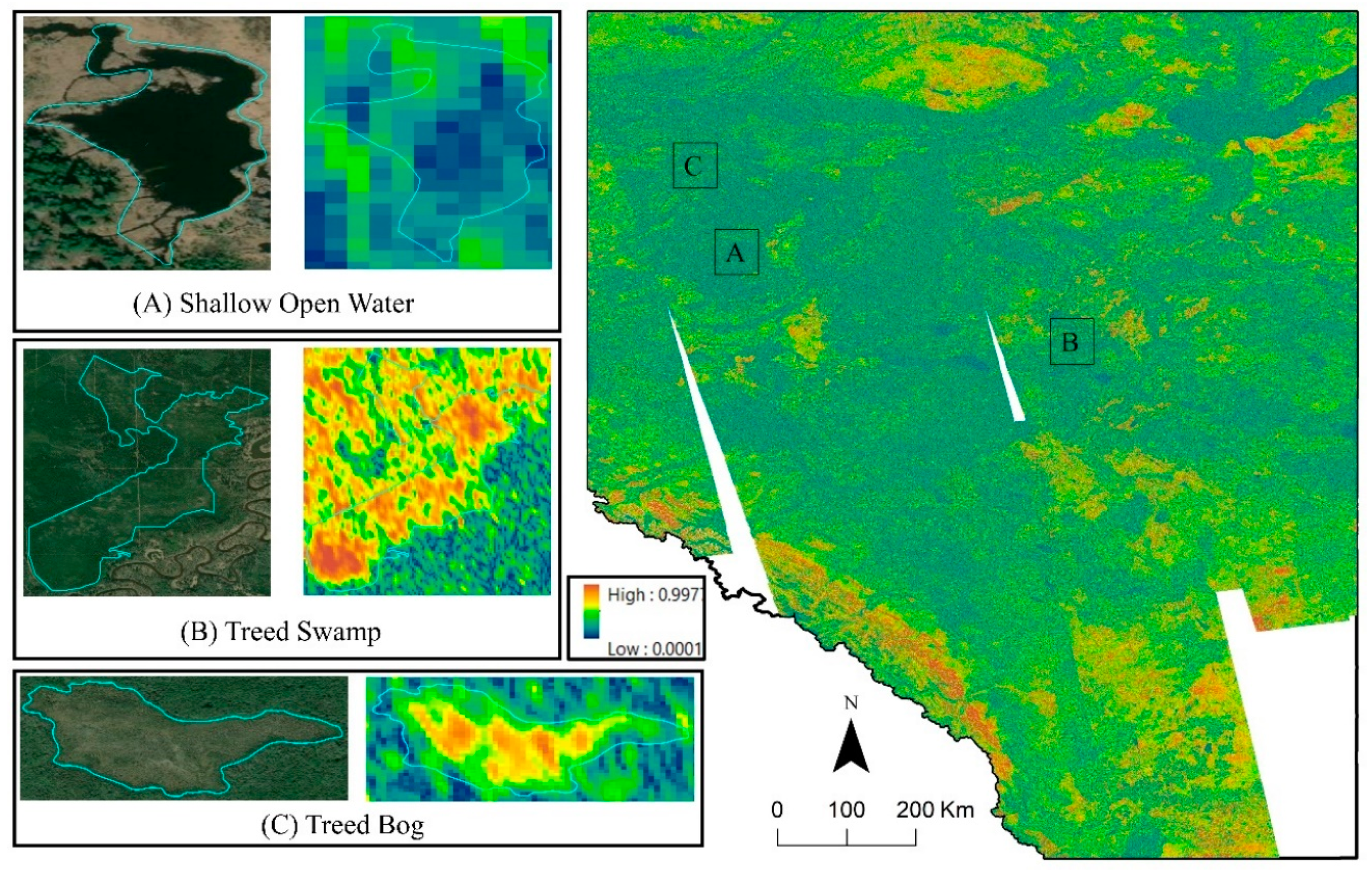
3.1. Monthly Coherence Change

Figure 5 illustrates the detailed monthly coherence products of the four categories. For instance, for the first category, the averaged coherence values of all seven wetland classes (see Table 1) were calculated for each monthly InSAR pair. According to Figure 5a, the coherence of all wetland classes, except Shallow Open Water (i.e., Category 1) showed a V-shaped trend over time, with the lowest value during the summer season. Wetlands had a good coherence of 0.5 in May when water is present under the vegetation due to snowmelt as well as lower density of tree canopies. Thereafter, there was a downward trend in the coherence to around a value of 0.3 in July. Finally, coherence values increased up to 0.6 in October when vegetation are relatively sparse.

Figure 5b compares the coherence of wetlands for Category 2. The Treed Wetland class was more coherent compared to the Open Wetland, leading to a suitable separability between the two classes. Moreover, the Treed Wetland class represented higher coherence when there was water beneath the trees in September and October.

With a more detailed inspection of the subclasses of Category 3 (Figure 5c), the Treed Bog was the subclass, which showed a distinguishable trend with the highest coherence values as opposed to the other subclasses. The coherence of this class decreased by 0.2 in July, following a considerable increase to approximately 0.75 in October. The Swamp and Marsh classes showed similar coherence trends over time. Consequently, it was difficult to distinguish these two classes based on InSAR coherence in Category 3.

With a close look at Category 4 (Figure 5d), Treed Bog, Treed Swamp, Treed Fen, and Open Fen had the highest coherence values, respectively. Among the Category 4 classes, the Shallow Open Water had the lowest coherence level (mainly noise) below 0.3.

3.2. Seasonal Coherence Change

The coherence values of different wetland classes at three seasons (different water levels and canopy closure of the species) are illustrated in Figure 6. Similar trends to Figure 4 were obtained for seasonal analysis. The results demonstrated that each class provided a similar coherence seasonal trend with the highest value during spring and fall seasons, making a clear V-shape pattern for coherency. The coherence was at the lowest level for the interferometric pairs during the summer season. However, the Shallow Open Water class did not follow this pattern and had a very low steady coherence trend during the seasons. Suitable distinguishing trends can be seen between the Treed Wetland and Open Wetland classes according to Figure 6b. Moreover, most of the wetland classes maintained coherence in the spring and fall seasons (Figure 6c). Overall, treed wetlands were more coherent than open ones. For instance, Treed Bog had the highest coherence values. The Treed Swamp and Treed Fen classes showed similar coherence values during different seasons, making them difficult to be discriminated based on coherence values in different seasons.

3.3. Leaf-On/Off Coherence Change

Leaf-on/off scenario was selected to investigate the canopy effect on wetlands coherence values. Figure 7 illustrates the leaf-on/off seasons versus annual coherence data for each wetland class. The interferometric pairs during the leaf-off season were more coherent for wetland classes compared to the leaf-on season (see Figure 7a). Coherence was preserved more for Treed Wetland, in which the coherence values were approximately higher than those of Open Wetland by 0.2 (Figure 7b). The highest coherence level was for the Treed Bog class, which showed a value of 0.75 during the leaf-off season. Following this, the Swamp and Fen classes maintained good coherence during September-October (Figure 7c). In summary, wetland classes preserved coherence during the leaf-off season while showing lower coherence values during the leaf-on season.

4. Discussion

4.1. Findings

Based on the results, coherence products can be effectively applied to discriminate wetland classes. The results showed that the Treed Wetland and Open Wetland classes could be easily distinguished using InSAR coherence products. This was because there was always a considerable difference in coherence levels between these two classes. Among the Treed Wetland classes, Treed Bog was more separable due to the high coherence values. However, the possibility of separating the Marsh, Swamp, and Fen classes based on coherence products should be further investigated. These were also illustrated using the violin plots where there are considerable overlaps between the coherence values of some of the wetland classes (see Figure 8). These results demonstrated that discriminating some of wetlands using coherence products is still challenging. For example, according to Figure 8, although the mean coherence values of the Bog and Marsh classes indicated good separability, the Fen and Swamp wetland classes had overlaps in coherence mean values, making it difficult to distinguish them using coherence information. Overall, it should be noted that wetlands are complex environments with similar spectral characteristics and, thus, distinguishing different wetland classes with other type of remote sensing data (e.g., optical and SAR data) is also difficult [10,50].

In this study, all wetland classes showed the lowest degree of coherence in summer. However, Shallow Open Water was the only wetland type, which provided no adequate coherence information. Shallow Open Water is a wetland with water depth of less than 2 m. Smooth water bodies react like a specular surface, reflecting the SAR signal away from the sensor, resulting in decorrelation. Furthermore, temporal decorrelations, induced by wind and precipitation, may change the water surface roughness, leading to a lower degree of coherence and noisy information [51].

The Treed Bog class showed the highest degree of coherency, followed by Treed Fen and Treed Swamp, respectively. The main reason for relatively lower coherence for the Treed Swamp class could be related to the higher density in the canopy of this class, which caused less penetration of the C-band through the dense canopies. Moreover, since the only water source of bogs is precipitation [52], a smoother water surface was probably formed compared to Treed Fen which can have multiple water sources. Therefore, the smoother water surface of Treed Bog led to higher double-bounce scattering values and, consequently, higher coherence values. The other reason might be due to the less dense canopy and understory vegetation in bogs compared to fens, resulting in less volume scattering contribution for the Treed Bog class.

Open wetlands decorrelated faster over a short period, making them incoherent classes most of the time. However, during flooding, double-bounce scattering can occur between the surface of the water and the stems/roots of vegetation. For example, the Marsh class showed much higher coherence values during fall. This may also be a result of plant growth of the herbaceous vegetation over the summer along with the rising water level.

The seasonal pattern of high coherence in spring, low in summer/leaf-on, and increasing in fall/leaf-off indicated coherence as a practical value for wetland change analysis (i.e., CCD) as well as for investigating the possibility of hydroperiod for inundated vegetation. The fall/leaf-off season relatively indicated higher coherence due to less canopy closure, and water level changes. The double-bounce backscattering becoming dominant in this season, indicating interactions between the water surface and trunks or emergent vegetation. This was similar for spring when there was water beneath the vegetation due to snow melting and a less developed canopy. At this point, the highest coherence levels belonged to the Treed Wetland class compared to the herbaceous/open species. Prominently, a rise in the water level improved the possibility of double-bounce scattering for flooded vegetation.

When there is dense vegetation (i.e., during the summer season), the dominant scattering mechanism is volume backscattering. As a result, the double-bouncing effect was limited and, thus, wetland classes lost coherence.

4.2. Future Works

As discussed in Section 2.2, a large amount of photo-interpreted reference samples collected from 2010 to 2016 over the entire Alberta were employed in this study. Although these datasets are the best available from the study area, they contain multiple errors and, this negatively affected the results. Although the reference samples were slightly refined, more detailed analyses should be performed in future to ensure the correct reference samples are utilized for coherence analysis. For example, all old samples (e.g., those collected in 2010 and 2011) should be interpreted again to ensure that wetland types or their boundaries have not been changed, especially in areas of with rapid human development. Moreover, the reference samples should be carefully removed from the analysis based on bad weather conditions and ice/snow presence.

In this study, all coherence measurements of the province of Alberta were averaged within the ABMI’s reference polygons at different times/locations for each wetland subclass (Table 1). Subsequently, all the coherence data of subclasses were also averaged to obtain the averaged coherence values for the main classes (e.g., Treed Wetland and Open Wetland). Additionally, for each date scenario (Section 2.5), one more averaging was applied to the measurements. It was observed that all of these averaging steps made coherence patterns and values show a lower degree and, thus, could negatively affect the real coherence information of the wetlands. Therefore, analyzing the coherence values for different locations, times, and subclasses separately may provide more accurate information about the advantages of InSAR coherency for wetland classification and change analysis.

The involvement of the incorrect reference samples and averaging the coherence measurements over different classes, times, and locations could be the main reason for the discrepancy between the results of this study and those reported by other studies. For example, it was reported that coherence values over the flooded marsh areas were relatively high due to higher double-bounce backscattering values [15,17]. However, the results of this study showed relatively low coherence values for the Marsh class. Although these results might be due to the different vegetation characteristics of marsh at different locations, future studies should initially revise the reference samples more comprehensively and avoid too many averaging steps to investigate the results behind this discrepancy in more detail.

In this study, coherence products were generated from the C-band Sentinel-1 data. Shorter wavelengths produce more surface scattering and stronger backscattering from small-scale surface roughness. However, returns in longer wavelengths (e.g., L-band) are less sensitive to small scatterers and small-scale roughness. Moreover, since the longer wavelengths have higher penetration capability, they are less sensitive to surface features that mask more relevant details in the coherence products [3,28,29]. Therefore, the use of L-band data for wetlands and/or flooded vegetations benefits from the double-bounce effect due to deeper penetration into the dense canopies. Future studies should use L-band data (e.g., those acquired by ALOS-4 and NASA-ISRO (NISAR)) along with Sentinel-1 C-band data to provide a more comprehensive information about wetland coherence and its advantages and limitations for wetland classification and change analysis.

In this study, the VV-polarized data of Sentinel-1 were utilized. It has been argued that flooded wetland areas are easier to identify using co-polarized data rather than cross-polarized data. The HH polarization is also preferred among co-polarized data due to its reduced sensitivity to water surface and more sensitivity to double-bounce scattering [3,16]. Therefore, it is suggested to investigate the coherence products generated from the HH polarization to make a more comprehensive conclusion about the application of coherence data for wetland mapping and monitoring.

Although coherence products are helpful for wetland mapping and monitoring, better results can be obtained by combining these products with SAR amplitude data and parameters generated from different decomposition methods. For instance, multi-temporal polarimetric data may be useful to differentiate classes with different scattering mechanisms by polarimetric decomposition methods. SAR intensity is a function of different factors, including surface/target features, vegetation height, density, and biomass [53]. The more signal reflects to the satellite, the more positive the intensity is. For wetlands, the SAR backscattering variations correlate with hydrology regimes, vegetation types, and soil wetness [29]. Therefore, a combination of intensity data with the coherence measurements should provide better wetland classification and change analysis results.

In this study, the coherence values were extracted to visually evaluate the separability of different wetland classes and their trends. However, various automatic statistical tests (e.g., T- and U-tests) can be used instead of visual interpretation of the coherence values to investigate the separability of wetland classes in more depth [10,50].

Most of the analyses performed in this study were statistical analyses based on the extracted coherence values. Future studies should investigate these data further in terms of the spatial distribution of coherence values. For example, coherence products (e.g., mean and standard deviation values) can be used along with the amplitude data to produce different false color composite products, and spatially investigate their applications for wetland classification. Various maps can also be produced based on the multi-temporal coherence products to investigate the effectiveness of these time-series products for wetland change analysis [15,17,54].

It is possible to develop coherence-based indices to classify wetlands by analyzing the coherence values of different wetland classes both in the single- and multi-date coherence products (i.e., Figure 4, Figure 5 and Figure 6). Moreover, 2D and 3D spaces generated from different single- and multi-date coherence/amplitude values can be constructed to develop coherence indices for wetland mapping and change analysis [15].

As discussed, wetlands are very dynamic and the water level within wetlands can considerably change over time due to several factors, such as precipitation. In the short term, rain can cause flooding, making changes in the appearance of wetlands within days. In the long term, wetlands can change from one type to another or be disturbed hydrologically [3]. Since coherence values change due to water level, they can be effectively used for hydroperiod in wetland areas, especially over open wetlands where SAR signals can penetrate [55].

Coherence depends on spatio-temporal baselines of InSAR pairs. Considering same satellite data with suitable small perpendicular baselines, the temporal baseline could play an essential role in coherence level. Different temporal baselines can be used in creating interferometric pairs to calculate coherence. Generally, coherence decreases as the temporal baseline increases due to seasonal canopy variation [16,28]. At the same time, increasing in water level can enhance the double-bouncing scattering. In this study, the Sentinel-1 coherence products were generated based on 12-days baseline data. However, considering the different patterns of wetland changes in Canada, it is suggested to produce coherence products with different baselines to investigate the dynamicity of wetlands in more detail.

Wetlands can be influenced by freezing/permafrost, causing soil degradation and, thus, wetland type transition. Coherence products can be used to detect freeze/thaw transition areas [15]. Therefore, future studies should investigate the effects of these events on coherence degrees and the applicability of coherence products for detecting freeze/thaw transition areas.

5. Conclusions

In this study, the potential of the InSAR coherence products generated from Sentinel-1 C-band data over a large province in Canada (i.e., Alberta) was investigated for wetland class separability and trend analysis. It was observed that coherence maps could be useful for wetland classification because several wetland types were easily distinguishable using InSAR coherence products. For example, the Treed Bog, which is usually challenging to be discriminated in optical satellite imagery, could be easily distinguished from other wetland types. Generally, treed wetlands showed the highest degree of coherence due to the trunks and water beneath, resulting in double-bouncing signals. Moreover, a V-shaped trend was observed when analyzing the monthly, seasonal, and leaf-on/off coherence products. In fact, coherence was relatively high in early spring and it then slightly decreased to its minimum value in July and, subsequently, increased to a maximum value on October. This trend was most probably due to changes in the vegetation density. We also discussed the limitations of the study and suggested several solutions for future studies. Future studies should comprehensively revise the reference samples and then, utilize the generated coherence products for various applications, including wetland classification, CCD, analyzing the hydroperiod pattern of wetlands, developing new coherence indices, and detecting freeze/thaw transition areas.

References

- Riley, W.J.; Subin, Z.M.; Lawrence, D.M.; Swenson, S.C.; Torn, M.S.; Meng, L.; Mahowald, N.M.; Hess, P. Barriers to predicting changes in global terrestrial methane fluxes: Analyses using CLM4Me, a methane biogeochemistry model integrated in CESM. Biogeosciences 2011, 8, 1925–1953. [Google Scholar] [CrossRef] [Green Version]
- Mahdavi, S.; Salehi, B.; Huang, W.; Amani, M.; Brisco, B. A PolSAR change detection index based on neighborhood information for flood mapping. Remote Sens. 2019, 11, 1854. [Google Scholar] [CrossRef] [Green Version]
- Mahdavi, S.; Salehi, B.; Granger, J.; Amani, M.; Brisco, B.; Huang, W. Remote sensing for wetland classification: A comprehensive review. GISci. Remote Sens. 2018, 55, 623–658. [Google Scholar] [CrossRef]
- Schmitt, A.; Brisco, B. Wetland monitoring using the curvelet-based change detection method on polarimetric SAR imagery. Water 2013, 5, 1036–1051. [Google Scholar] [CrossRef]
- Adeli, S.; Salehi, B.; Mahdianpari, M.; Quackenbush, L.J.; Brisco, B.; Tamiminia, H.; Shaw, S. Wetland monitoring using SAR data: A meta-analysis and comprehensive review. Remote Sens. 2020, 12, 2190. [Google Scholar] [CrossRef]
- Elhadi, M.I.A.; Mutanga, O.; Rugege, D.; Ismail, R. Field spectrometry of papyrus vegetation (Cyperus papyrus L.) in swamp wetlands of St Lucia, South Africa. In Proceedings of the 2009 IEEE International Geoscience and Remote Sensing Symposium, Cape Town, South Africa, 12–17 July 2009; Volume 4, p. 260. [Google Scholar]
- Amani, M.; Mahdavi, S.; Afshar, M.; Brisco, B.; Huang, W.; Mohammad Javad Mirzadeh, S.; White, L.; Banks, S.; Montgomery, J.; Hopkinson, C. Canadian Wetland Inventory using Google Earth Engine: The First Map and Preliminary Results. Remote Sens. 2019, 11, 842. [Google Scholar] [CrossRef] [Green Version]
- Kaplan, G.; Avdan, U. Monthly analysis of wetlands dynamics using remote sensing data. ISPRS Int. J. Geo-Inf. 2018, 7, 411. [Google Scholar] [CrossRef] [Green Version]
- Zhao, J.; Niu, Y.; Lu, Z.; Yang, J.; Li, P.; Liu, W. Applicability Assessment of Uavsar Data in Wetland Monitoring: A Case Study of Louisiana Wetland. ISPRS Int. Arch. Photogramm. Remote Sens. Spat. Inf. Sci. 2018, 2375–2378. [Google Scholar] [CrossRef] [Green Version]
- Amani, M.; Salehi, B.; Mahdavi, S.; Brisco, B. Separability analysis of wetlands in Canada using multi-source SAR data. GISci. Remote Sens. 2019, 56, 1233–1260. [Google Scholar] [CrossRef]
- Hird, J.; DeLancey, E.; McDermid, G.; Kariyeva, J. Google Earth Engine, Open-Access Satellite Data, and Machine Learning in Support of Large-Area Probabilistic Wetland Mapping. Remote Sens. 2017, 9, 1315. [Google Scholar] [CrossRef] [Green Version]
- Salvia, M.; Franco, M.; Grings, F.; Perna, P.; Martino, R.; Karszenbaum, H.; Ferrazzoli, P. Estimating flow resistance of wetlands using SAR images and interaction models. Remote Sens. 2009, 1, 992–1008. [Google Scholar] [CrossRef] [Green Version]
- DeLancey, E.R.; Kariyeva, J.; Cranston, J.; Brisco, B. Monitoring Hydro Temporal Variability in Alberta, Canada with Multi-Temporal Sentinel-1 SAR Data. Can. J. Remote Sens. 2018, 44, 1–10. [Google Scholar] [CrossRef]
- Brisco, B.; Shelat, Y.; Murnaghan, K.; Montgomery, J.; Fuss, C.; Olthof, I.; Hopkinson, C.; Deschamps, A.; Poncos, V. Evaluation of C-Band SAR for Identification of Flooded Vegetation in Emergency Response Products. Can. J. Remote Sens. 2019, 45, 73–87. [Google Scholar] [CrossRef]
- Brisco, B.; Ahern, F.; Murnaghan, K.; White, L.; Canisus, F.; Lancaster, P. Seasonal change in wetland coherence as an aid to wetland monitoring. Remote Sens. 2017, 9, 158. [Google Scholar] [CrossRef] [Green Version]
- Tsyganskaya, V.; Martinis, S.; Marzahn, P.; Ludwig, R. SAR-based detection of flooded vegetation—A review of characteristics and approaches. Int. J. Remote Sens. 2018, 39, 2255–2293. [Google Scholar] [CrossRef]
- Canisius, F.; Brisco, B.; Murnaghan, K.; Van Der Kooij, M.; Keizer, E. SAR Backscatter and InSAR Coherence for Monitoring Wetland Extent, Flood Pulse and Vegetation: A Study of the Amazon Lowland. Remote Sens. 2019, 11, 720. [Google Scholar] [CrossRef] [Green Version]
- DeLancey, E.R.; Brisco, B.; Canisius, F.; Murnaghan, K.; Beaudette, L.; Kariyeva, J. The Synergistic Use of RADARSAT-2 Ascending and Descending Images to Improve Surface Water Detection Accuracy in Alberta, Canada. Can. J. Remote Sens. 2019, 45, 759–769. [Google Scholar] [CrossRef]
- Alsdorf, D.E.; Smith, L.C.; Melack, J.M. Amazon floodplain water level changes measured with interferometric SIR-C radar. IEEE Trans. Geosci. Remote Sens. 2001, 39, 423–431. [Google Scholar] [CrossRef]
- Lee, H.; Yuan, T.; Yu, H.; Jung, H.C. Interferometric SAR for wetland hydrology: An overview of methods, challenges, and trends. IEEE Geosci. Remote Sens. Mag. 2020, 8, 120–135. [Google Scholar] [CrossRef]
- Alsdorf, D.E.; Melack, J.M.; Dunne, T.; Mertes, L.A.K.; Hess, L.L.; Smith, L.C. Interferometric radar measurements of water level changes on the Amazon flood plain. Nature 2000, 404, 174–177. [Google Scholar] [CrossRef]
- Foroughnia, F.; Nemati, S.; Maghsoudi, Y.; Perissin, D. An iterative PS-InSAR method for the analysis of large spatio-temporal baseline data stacks for land subsidence estimation. Int. J. Appl. Earth Obs. Geoinf. 2019, 74, 248–258. [Google Scholar] [CrossRef]
- Ranjgar, B.; Razavi-Termeh, S.V.; Foroughnia, F.; Sadeghi-Niaraki, A.; Perissin, D. Land Subsidence Susceptibility Mapping Using Persistent Scatterer SAR Interferometry Technique and Optimized Hybrid Machine Learning Algorithms. Remote Sens. 2021, 13, 1326. [Google Scholar] [CrossRef]
- Olen, S.; Bookhagen, B. Applications of SAR interferometric coherence time series: Spatiotemporal dynamics of geomorphic transitions in the south-central Andes. J. Geophys. Res. Earth Surf. 2020, 125, e2019JF005141. [Google Scholar] [CrossRef]
- Yuan, M.; Xie, C.; Shao, Y.; Xu, J.; Cui, B.; Liu, L. Retrieval of water depth of coastal wetlands in the Yellow River Delta from ALOS PALSAR backscattering coefficients and interferometry. IEEE Geosci. Remote Sens. Lett. 2016, 13, 1517–1521. [Google Scholar] [CrossRef]
- Zebker, H.A.; Villasenor, J. Decorrelation in interferometric radar echoes. IEEE Trans. Geosci. Remote Sens. 1992, 30, 950–959. [Google Scholar] [CrossRef] [Green Version]
- Agram, P.S.; Simons, M. A noise model for InSAR time series. J. Geophys. Res. Solid Earth 2015, 120, 2752–2771. [Google Scholar] [CrossRef]
- Mohammadimanesh, F.; Salehi, B.; Mahdianpari, M.; Brisco, B.; Motagh, M. Wetland water level monitoring using interferometric synthetic aperture radar (InSAR): A review. Can. J. Remote Sens. 2018, 44, 247–262. [Google Scholar] [CrossRef]
- Mohammadimanesh, F.; Salehi, B.; Mahdianpari, M.; Brisco, B.; Motagh, M. Multi-temporal, multi-frequency, and multi-polarization coherence and SAR backscatter analysis of wetlands. ISPRS J. Photogramm. Remote Sens. 2018, 142, 78–93. [Google Scholar] [CrossRef]
- Santoro, M.; Wegmuller, U.; Askne, J.I.H. Signatures of ERS–Envisat interferometric SAR coherence and phase of short vegetation: An analysis in the case of maize fields. IEEE Trans. Geosci. Remote Sens. 2009, 48, 1702–1713. [Google Scholar] [CrossRef]
- Cartus, O.; Santoro, M.; Wegmüller, U.; Labrière, N.; Chave, J. Sentinel-1 Coherence for Mapping Above-Ground Biomass in Semiarid Forest Areas. IEEE Geosci. Remote Sens. Lett. 2021. [Google Scholar] [CrossRef]
- Santoro, M.; Askne, J.I.H.; Wegmuller, U.; Werner, C.L. Observations, modeling, and applications of ERS-ENVISAT coherence over land surfaces. IEEE Trans. Geosci. Remote Sens. 2007, 45, 2600–2611. [Google Scholar] [CrossRef]
- Mirzaee, S.; Motagh, M.; Arefi, H.; Nooryazdan, A. Phenological tracking og agricultural feilds investigated by using dual polarimetry tanDEM-X images. Int. Arch. Photogramm. Remote Sens. Spat. Inf. Sci. 2015, 40, 73. [Google Scholar] [CrossRef] [Green Version]
- Hong, S.H.; Wdowinski, S.; Kim, S.W.; Won, J.S. Multi-temporal monitoring of wetland water levels in the Florida Everglades using interferometric synthetic aperture radar (InSAR). Remote Sens. Environ. 2010, 114, 2436–2447. [Google Scholar] [CrossRef]
- Xie, C.; Xu, J.; Shao, Y.; Cui, B.; Goel, K.; Zhang, Y.; Yuan, M. Long term detection of water depth changes of coastal wetlands in the Yellow River Delta based on distributed scatterer interferometry. Remote Sens. Environ. 2015, 164, 238–253. [Google Scholar] [CrossRef] [Green Version]
- Minotti, P.G.; Rajngewerc, M.; Santoro, V.A.; Grimson, R. Evaluation of SAR C-band interferometric coherence time-series for coastal wetland hydropattern mapping. J. S. Am. Earth Sci. 2021, 106, 102976. [Google Scholar] [CrossRef]
- Liao, T.H.; Simard, M.; Denbina, M.; Lamb, M.P. Monitoring water level change and seasonal vegetation change in the coastal wetlands of louisiana using L-band time-series. Remote Sens. 2020, 12, 2351. [Google Scholar] [CrossRef]
- By, C.; Pettapiece, D.J.D. and W.W. Natural Regions and Subregions of Alberta: Natural Regions Committee; Government of Alberta: Edmonton, AB, Canada, 2016; ISBN 0778545725. [Google Scholar]
- DeLancey, E.R.; Simms, J.F.; Mahdianpari, M.; Brisco, B.; Mahoney, C.; Kariyeva, J. Comparing Deep Learning and Shallow Learning for Large-Scale Wetland Classification in Alberta, Canada. Remote Sens. 2019, 12, 2. [Google Scholar] [CrossRef] [Green Version]
- NASA. ASF. Available online: https://search.asf.alaska.edu (accessed on 15 March 2021).
- Hanssen, R.F. Radar Interferometry: Data Interpretation and Error Analysis; Springer Science & Business Media: New York, NY, USA, 2001; Volume 2, ISBN 0792369459. [Google Scholar]
- CPOD. Sentinel-1 POD Products Performance; Copernicus Sentinel-1, -2 and -3 Precise Orbit Determination Service (Sentinelspod); European Space Agency: Paris, France, 2019; Available online: https://sentinel.esa.int/documents/247904/3455957/Sentinel-1-POD-Products-Performance.pdf (accessed on 15 March 2021).
- Mallorquí, J.; Mora, O.; Blanco, P.; Broquetas, A. Linear and Non-Linear Long-Term Terrain Deformation with Dinsar (CPT: Coherent Pixels Technique). In Proceedings of the Fringe 2003 Workshop, Frascati, Italy, 1–5 December 2003. [Google Scholar]
- Zebker, H.A.; Rosen, P.A.; Hensley, S. Atmospheric effects in interferometric synthetic aperture radar surface deformation and topographic maps. J. Geophys. Res. Solid Earth 1997, 102, 7547–7563. [Google Scholar] [CrossRef]
- Pepe, A.; Calò, F. A Review of Interferometric Synthetic Aperture RADAR (InSAR) Multi-Track Approaches for the Retrieval of Earth’s Surface Displacements. Appl. Sci. 2017, 7, 1264. [Google Scholar] [CrossRef] [Green Version]
- Goldstein, R.M.; Werner, C.L. Radar interferogram filtering for geophysical applications. Geophys. Res. Lett. 1998, 25, 4035–4038. [Google Scholar] [CrossRef] [Green Version]
- Marinkovic, P.; Ketelaar, G.; Leijen, F.V.; Hanssen, R. InSAR Quality Control: Analysis of Five Years of Corner Reflector Time Series. In Proceedings of the Fringe 2007 Workshop, Frascati, Italy, 26–30 November 2007. [Google Scholar]
- Gatelli, F.; Monti Guamieri, A.; Parizzi, F.; Pasquali, P.; Prati, C.; Rocca, F. The wavenumber shift in SAR interferometry. IEEE Trans. Geosci. Remote Sens. 1994, 32, 855–865. [Google Scholar] [CrossRef] [Green Version]
- Yague-Martinez, N.; De Zan, F.; Prats-Iraola, P. Coregistration of Interferometric Stacks of Sentinel-1 TOPS Data. IEEE Geosci. Remote Sens. Lett. 2017, 14, 1002–1006. [Google Scholar] [CrossRef] [Green Version]
- Amani, M.; Salehi, B.; Mahdavi, S.; Brisco, B. Spectral analysis of wetlands using multi-source optical satellite imagery. ISPRS J. Photogramm. Remote Sens. 2018, 144, 119–136. [Google Scholar] [CrossRef]
- Lu, Z.; Kwoun, O. Radarsat-1 and ERS InSAR Analysis over Southeastern Coastal Louisiana: Implications for Mapping Water-Level Changes Beneath Swamp Forests. IEEE Trans. Geosci. Remote Sens. 2008, 46, 2167–2184. [Google Scholar] [CrossRef]
- Mahdavi, S.; Salehi, B.; Amani, M.; Granger, J.E.; Brisco, B.; Huang, W.; Hanson, A. Object-Based Classification of Wetlands in Newfoundland and Labrador Using Multi-Temporal PolSAR Data. Can. J. Remote Sens. 2017, 43, 432–450. [Google Scholar] [CrossRef]
- Kim, S.-W.; Wdowinski, S.; Amelung, F.; Dixon, T.H.; Won, J.-S. Interferometric Coherence Analysis of the Everglades Wetlands, South Florida. IEEE Trans. Geosci. Remote Sens. 2013, 51, 5210–5224. [Google Scholar] [CrossRef]
- Shang, J.; Liu, J.; Poncos, V.; Geng, X.; Qian, B.; Chen, Q.; Dong, T.; Macdonald, D.; Martin, T.; Kovacs, J.; et al. Detection of Crop Seeding and Harvest through Analysis of Time-Series Sentinel-1 Interferometric SAR Data. Remote Sens. 2020, 12, 1551. [Google Scholar] [CrossRef]
- Battaglia, M.J.; Banks, S.; Behnamian, A.; Bourgeau-Chavez, L.; Brisco, B.; Corcoran, J.; Chen, Z.; Huberty, B.; Klassen, J.; Knight, J.; et al. Multi-Source EO for Dynamic Wetland Mapping and Monitoring in the Great Lakes Basin. Remote Sens. 2021, 13, 599. [Google Scholar] [CrossRef]