Article

Pass-by-Pass Ambiguity Resolution in Single GPS Receiver PPP Using Observations for Two Sequential Days: An Exploratory Study

1
GNSS Research Center, Wuhan University, 129 Luoyu Road, Wuhan 430079, China
2
Nottingham Geospatial Institute, The University of Nottingham, Nottingham NG7 2TU, UK
3
The Sino-UK Geospatial Engineering Centre, Nottingham NG8 1NA, UK
4
Global Geospatial Engineering Ltd., Nottingham NG8 1NA, UK
5
School of Geodesy and Geomatics, Wuhan University, 129 Luoyu Road, Wuhan 430079, China
*
Author to whom correspondence should be addressed.
Remote Sens. 2021, 13(18), 3728; https://doi.org/10.3390/rs13183728
Submission received: 23 August 2021 / Accepted: 15 September 2021 / Published: 17 September 2021

Abstract

:
“Pass-by-pass” or “track-to-track” ambiguity resolution removes Global Navigation Satellite System (GNSS) satellite hardware delays between adjacent undifferenced (UD) ambiguities, which is often applied in precise orbit determination (POD) for Low Earth Orbit (LEO) satellites to improve the accuracy of orbits. In this study, we carried out an exploratory study to use the “pass-by-pass” ambiguity resolution by differencing the undifferenced ambiguity candidates for two adjacent passes in sidereal days for a single Global Positioning System (GPS) receiver static Precise Point Positioning (PPP). Using the GPS observations from 132 globally distributed reference stations of International GPS Service (IGS), we find that 99.08% wide-lane (WL) and 97.83% narrow-lane (NL) double-difference ambiguities formed by the “pass-by-pass” method for all stations can be fixed to their nearest integers within absolute fractional residuals of 0.2 cycles. These proportions are higher than the corresponding values of network solution with multiple receivers with 97.39% and 91.20%, respectively. About 97% to 98% of ambiguities can be fixed finally on average. The comparison of the estimated station coordinates with the IGS weekly solutions reveals that the Root Mean Square (RMS) in East and North directions are 2-4 mm and is about 6 mm in the Up direction. For hourly data, it is found that the mean positioning accuracy improvement can achieve to about 10% after ambiguity resolution. From a dam deformation monitoring application, it shows that the fixing rate of WL and NL ambiguity can be closed to 100% and higher than 90%, respectively. The time series generated by PPP are also in agreement with the short baseline solutions.

1. Introduction

The Global Positioning System (GPS) is nowadays widely used in Earth scientific explorations, such as tectonic motion, glacial isostatic adjustment, monitoring strong or slow ground motion due to earthquakes [1] and volcanoes [2], and engineering applications, such as monitoring the health conditions of dams and bridges [3,4], and ground subsidence [5]. In most of these applications, baselines are generally formed between GPS stations to generate a network to eliminate the common errors in observation level using double-difference (DD) algorithm, such as ionospheric and tropospheric delays, satellite orbit errors and clock errors. The baselines can also assist the ambiguity resolution in un-difference (UD) modeling by mapping the UD ambiguities into a maximum set of independent DD-ambiguities. In this case, the uncalibrated phase delay originating in satellite and receiver could be canceled to recovery the natural integer feature of DD ambiguities [6,7,8].
Precise point positioning (PPP) employs only one receiver to realize high precise positioning results by applying improved satellite products. Compared with the baseline resolution in a network, the positioning model of PPP is simple, no correlations need to be introduced in the measurement variance-matrix, and all parameters will remain available in the UD model. However, the fractional cycle bias (FCB) caused by the uncalibrated phase delay cannot be eliminated in UD-ambiguity estimates of PPP. Only DD ambiguities have a natural integer feature and can be fixed [9,10]. Thus, for a single receiver PPP, the ambiguities have to be kept as float values. It has been confirmed that the float ambiguities will introduce amplified spurious signals into long-term positioning times series [11,12], and the noise of time series could be larger than the fixed solutions. The geophysical signals will be hard to extract or model in the realization of the reference frame and the dynamics of the earth.
Fortunately, there are several studies that have developed FCB correction technology, which can separate the biases of uncalibrated phase delay from integer ambiguities by applying improved satellite products [13,14]. Ge et al. [8] proposed a method by decomposing the UD ambiguities into wide-lane ambiguities and narrow-lane ones, and a single-difference between satellites could be applied to difference the receiver-dependent FCBs. Then, the satellite relevant FCBs of wide-lane and narrow-lane could be estimated by applying GPS observations of a reference network. For PPP application, ambiguity fixed solutions could be obtained with a single local receiver by correcting the wide-lane and narrow-lane FCBs. Laurichesse et al. [14] and Collins [15] proposed the integer recovery clock (IRC) model and the Decoupled Satellite Clock (DSC) model to identify the narrow-lane ambiguities as integers and fixed to integers before estimating clocks. In this way, the FCBs will be absorbed by clock products and provided to PPP users. Geng et al. [16] and Shi and Gao [17] proved that the two methods of ambiguities-fixed position estimates are theoretically equivalent. Teunissen and Khodabandeh [10] comprehensively compared the different formulations of these models and determined the transformational links between their PPP-RTK corrections [10].
Another method called “pass-by-pass” or “track-to-track” is to difference the hardware delays between adjacent UD ambiguities for the same GNSS-LEO pair, which was generally used in precise orbit determination (POD) of Low Earth Orbit (LEO) satellites [14,18,19]. The advantage of this method is that the ambiguities can be fixed for a single receiver without applying external FCB or IRC corrections. It should be noted that the hardware delay variations of a receiver need to be relatively stable between passes, so that the hardware delays of the receiver can be removed. The method has been successfully used in orbit determination of Sentinek-3A, SWARM satellites, and DLR’s GNSS orbit determination software tools [18,20]. However, the method is now often applied and analyzed in POD, and rare research focuses on its applicability and effectiveness in PPP, while it is applicable in PPP theoretically.
Therefore, in this paper, we carried out an exploratory study to use the “pass-by-pass” ambiguity resolution in single GPS receiver PPP by differencing the satellite-related hardware delays between undifferenced ambiguity candidates for two adjacent passes in sidereal days and the receiver-related ones between satellites. In the following sections, the basic principles of PPP and the “pass-by-pass” ambiguity resolution for a single GPS receiver will be presented first in Section 2. Then, Section 3 includes the assessment of the methods in ambiguity resolution and precision improvement using GPS observations of permanent stations from IGS and stations from a dam deformation monitoring system, and Section 4 shows the conclusions.

2. Methods

In this section, the observation models and parameter estimation will be firstly discussed. Then, the pass-by-pass ambiguity resolution and the data processing scheme will be mainly presented.

2.1. Observation Models

In GPS PPP models, the Ionosphere-Free (IF) combinations are often applied to eliminate the first-order ionospheric delays in the pseudorange and carrier-phase measurements. Therefore, the UD-observation equations of IF combinations of pseudorange and carrier-phase observations can be written as
{ P p ( i f ) i = ρ p i + c ( d t p d t i ) + T p i + e p ( i f ) i L p ( i f ) i = ρ p i + c ( d t p d t i ) + T p i + λ 1 N ˜ p ( i f ) i + ε p ( i f ) i ,
where i and p indicate satellite and receiver respectively; P is the original pseudorange observation and L is the carrier-phase measurement; λ 1 is the wavelength of the first frequency of GPS; ρ p i is the geometric distance from a satellite to the receiver; c is the speed of light; d t p and d t i are the clock errors of the receiver and satellite, respectively. T is the slant tropospheric delay. e and ε denote the measurement noise of GPS pseudorange and carrier-phase observations. N is the integer ambiguity, which is expressed from the relationship
N ˜ p ( i f ) i = N p ( i f ) i + ( ( B i b i ) ( B p b p ) ) λ 1 ,
where B p and B i are the receiver-dependent and satellite-dependent uncalibrated phase delays, and b i and b p are the corresponding uncalibrated pseudorange delays.
In the parameter estimation model, we used the precise orbit and clock products provided by IGS. The absolute phase centers, phase-wind up effects, and tidal loading displacement proposed by the International Terrestrial Reference Frame (ITRF) conventions 2003 were applied [8,21]. The estimated parameters in this study are position of the receiver, receiver clocks, zenith tropospheric delays (ZTD) and PPP ambiguities. Station coordinates are estimated with an initial constraint of 0.2 m. Receiver clock is estimated as white noise process for each epoch [8]. Zenith tropospheric delays are corrected by the Saastamoinen model for wet and dry hydrostatic delay with Global Mapping Function (GMF) [22], and the residual wet delays are estimated as piecewise constant function with a 1 h parameter interval.
If the corrections of receiver position parameters are denoted as vector x , ambiguity parameters as vector b and the time-related parameters receiver clock and ZTDs as vector u , the linearized observation equations for the visible satellites at epoch e can be written as
v e = A e x + B e b + C e u l e , P e ,
where A e , B e , and C e indicate coefficient matrices of x , b and u ; and P e is the weight matrix. Vector l e denotes the OMCs (i.e., observed minus computed measures with initial information) and v e contains mainly noise terms, including multipath and unmodeling errors. Therefore, the normal equation of the least squares model at this epoch is
[ A e T P e A e A e T P e B e A e T P e C e B e T P e B e B e T P e C e C e T P e C e ] [ x b u ] = [ A e T P e l e B e T P e l e C e T P e l e ] ,
If the observations in all epochs are accumulated into one final normal equation system, it could be
[ N x x N x b N x u N b b N b u N u u ] [ x b u ] = [ w x w b w u ] ,
where N and w indicate the elements accumulated from (3). The final solutions of the model after resolving with the least-squares method are as
[ x b u ] = [ Q x x Q x b Q x u Q b b Q b u Q u u ] [ w x w b w u ] ,
where Q denotes the variance-covariance matrix relating the elements in (5). If we use n and t to indicate the number of observations and the unknow parameters, the variance of unit weight or the variance factor σ 0 2 is calculated by
σ 0 2 = l T P l x T w x b T w b u T w u n t ,
It should be noted that this is the model of real-valued PPP solutions and it could be utilized as the basic model for ambiguity resolution.

2.2. Ambiguity Resolution

The ambiguity estimates we have obtained using the model mentioned above are real-valued. As proposed by Ge et al. [6], we divided the IF ambiguities estimates into wide-lane and narrow-lane terms as
N ˜ p ( i f ) i = g 1 + g N ˜ p ( n l ) i + g g 2 1 N ˜ p ( w l ) i ,
where g = f 1 / f 2 , and N ˜ p ( w l ) i and N ˜ p ( n l ) i denote the real-valued WL and NL ambiguities. The WL ambiguity can be estimated by the Hatch-Melbourne–Wübbena (HMW) [23,24,25] combination over the epochs of a data arc, where an arc means a continuous tracking without cycle-slips.
N ˜ ( w l ) = ( f 1 f 1 f 2 L 1 f 2 f 1 f 2 L 2 ) ( f 1 f 1 + f 2 P 1 + f 2 f 1 + f 2 P 2 ) λ ( w l ) ,
However, the WL ambiguity is biased by the satellite and receiver hardware bias as
N ˜ p ( w l ) i = N p ( w l ) i + δ η p ( w l ) + δ τ ( w l ) i ,
where N p ( w l ) i is the integer natural undifferenced ambiguity of satellite i , and δ τ ( w l ) i and δ η p ( w l ) are the hardware delays of a satellite and the receiver, respectively, which cannot be separated from the integer valued WL ambiguities. In baseline solutions, the double-differenced method can eliminate the biases to recovery the natural integer feature of WL ambiguity. Alternatively, for a single receiver situation, the single-differenced method is applied between satellites to cancel out the biases related to the receiver at first, and the satellite hardware biases are corrected by the FCB products which need to be estimated in advance using a regional or global network [8,21].
As is well-known the repeat period of the GPS constellation is 23 h 56 min plus 4 s, which is close to 24 h. In many high-precision GPS positioning applications, the GPS data is normally processed in the period of one day to remove site-related multipath effects. Therefore, for a ground-based receiver, there is only one entire arc for a GPS satellite for one station. However, two entire arcs can be observed for a satellite when the GPS observations for two sequential days are applied. If we processed the GPS data in two consecutive days, the station coordinates, station clocks, ZTD at stations will be estimated as normal and the carrier phase ambiguity parameters doubled taking the assumption that no cycle-slips exist. Thus, the float undifferenced WL ambiguities of satellite i in a session will be
{ N ˜ p ( w l ) , 1 i = N p ( w l ) , 1 i + δ η p ( w l ) , 1 + δ τ ( w l ) , 1 i N ˜ p ( w l ) , 2 i = N p ( w l ) , 2 i + δ η p ( w l ) , 2 + δ τ ( w l ) , 2 i
where the subscript of 1 and 2 indicate the day number of the ambiguity. Ge et al. [8] denoted that the WL FCBs were stable in a relatively long period and can be estimated and predicted and this means
δ τ ( w l ) , 1 i = δ τ ( w l ) , 2 i ,
Thus, the ambiguity estimates of a specific satellite can be removed between adjacent passes in two sidereal days to eliminate the satellite related hardware biases. Then, a difference can be applied between satellites as one normally does to cancel out the receiver related hardware biases δ η p ( w l ) . The DD WL ambiguity could be expressed as
Δ N ˜ p ( w l ) , 12 i , j = Δ N p ( w l ) , 12 i , j ,
Therefore, the DD WL ambiguity will have the natural integer feature. Figure 1 shows the detailed differential operations.
In order to give the fixable probability of the DD WL ambiguity, the decision function method is applied with the ambiguity estimate and variance [6,26]:
ξ = 1 i = 1 [ e r f c ( i | n N | 2 σ ) e r f c ( i + | n N | 2 σ ) ] ,
with
e r f c ( x ) = 2 π x e t 2 d t ,
where n is the ambiguity estimate that want to be fixed. σ is the variance of this ambiguity, and N is the nearest integer of n. Given a confidence level α , the ambiguity could be fixed with the probability ξ larger than 1 α , otherwise not. Usually, α is 0.1%. However, to prevent fixing to wrong ambiguity, if the fractional part of the ambiguity is larger than a threshold, e.g., 0.2 cycles, it cannot be fixed no matter how small its STD is.
If the WL ambiguity is fixed as Δ N ( w l ) , 12 i , j , the DD IF ambiguities Δ N ˜ ( i f ) , 12 i , j can be formed as the WL ambiguity does. Thus, the DD NL ambiguity can be derived from Equation (8) as
Δ N ˜ ( n l ) , 12 i j = g g + 1 Δ N ˜ ( i f ) , 12 i j 1 g 1 Δ N ( w l ) , 12 i j ,
In this case, the probability of being fixed to the nearest integer of DD NL ambiguities will be checked using Equation (14) and fixed in the same way as DD WL ambiguities.

2.3. Least-Squares Estimation with Fixed Ambiguities

After fixing the DD WL and NL ambiguities, we can apply the following equation to form the fixed DD IF ambiguities as
Δ N ( i f ) , 12 i j = g g 2 1 Δ N ( w l ) , 12 i j + g 1 + g Δ N ( n l ) , 12 i j ,
and treat the fixed IF ambiguity values as pseudo-observations in matrix
v b = D b b c , P b ,
where b c are the DD IF ambiguities with integer nature value, D is the ambiguity mapping matrix, and P b are the weights of the pseudo-observations for about 1010 [6]. With the constraints adding to the Normal Equation (NEQ) in Equation (5), the new NEQ can read as
[ N x x N x b N x u N ¯ b b N b u N u u ] [ x b u ] = [ w x w ¯ b w u ] ,
where
N ¯ b b = B T P B + D T P b D w ¯ b = B T P l + D T P b b c
Then, the previous model could be solved with the least-squares estimation, and the ambiguity-fixed PPP solutions can be obtained.
In summary, the FCBs can be eliminated by differencing the SD ambiguities parameters for a same satellite pair at two adjacent days, and the GPS ambiguity-fixed solution at a single receiver can be realized without applying FCB corrections. However, this method now is only usable in static PPP post-processing.

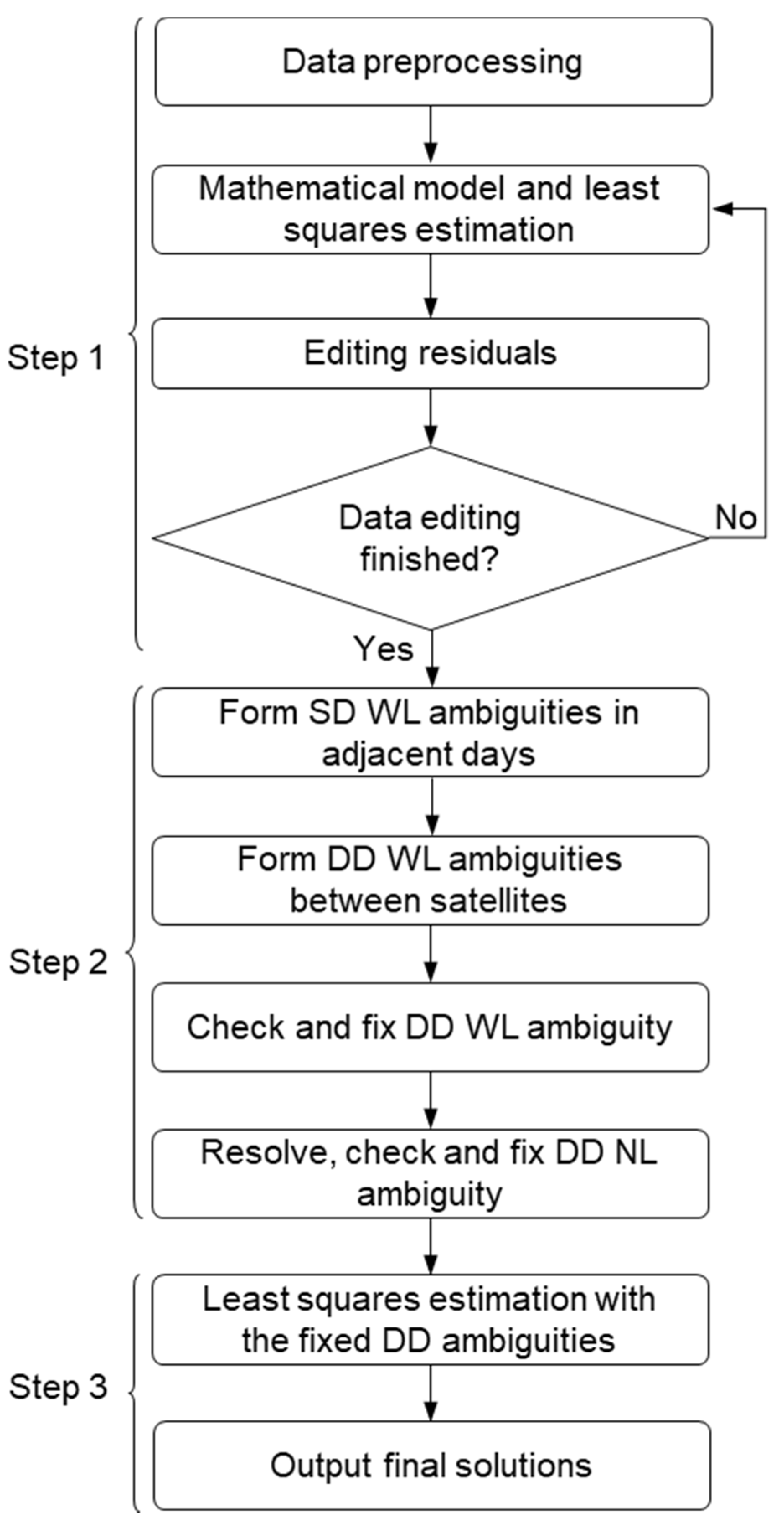
2.4. Data Processing Scheme

According to the methods mentioned above, the data processing scheme could be mainly divided into three steps which are shown in Figure 2, and the details are as follows:
  • The first step includes data preprocessing mathematical modelling, parameter estimation and residual editing. In data preprocessing, the data gaps and cycle-slips are detected based on the Turboedit algorithm [27]. Then, the code and carrier-phase observations are modelled with the IF combinations, and the parameters are estimated with the sequential least squares method to obtain the real-valued solution. It should be noted that we do not eliminate the ambiguity parameter as [7] did, because the number of parameters is not large for a single station.
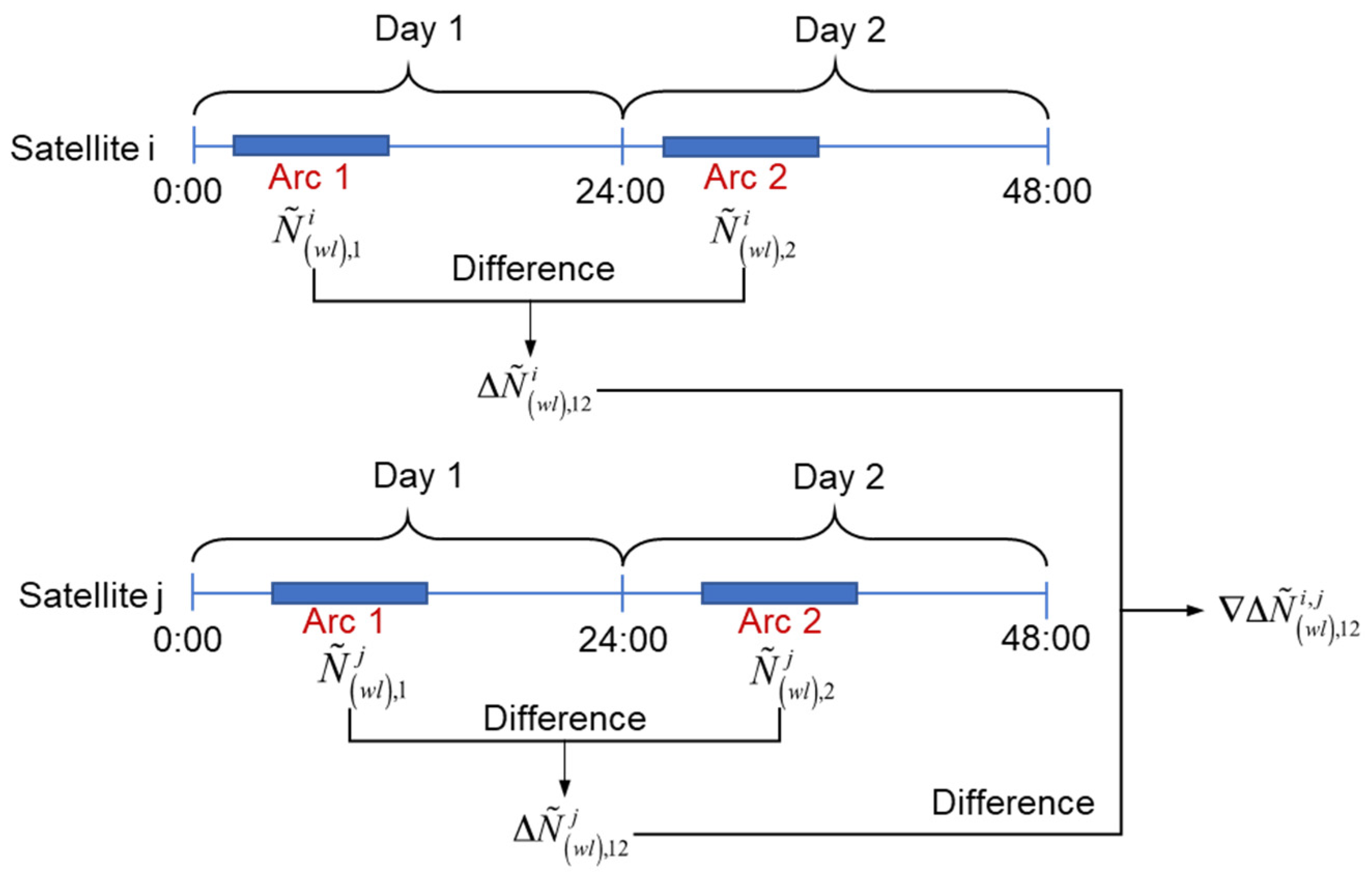
  • The second step is on the ambiguity resolution. Firstly, the un-differenced estimates of wide-lane ambiguities are derived from HMW combinations. Then, for each satellite, search the corresponding WL ambiguity for the second sidereal day through the start and end epochs plus 2864, and form the SD WL ambiguity. Note that, even though the specific GPS satellite has slightly different repeat periods [28,29], observations with 30s sampling rate would not have to consider the specific repeat period. However, for the higher sampling rates, such as less than 10s, the exact repeat period needs to be considered for the specific satellite. Next, the DD ambiguity is formed between satellites and inserted to Equation (14) to check whether the ambiguity can be successfully resolved. If it is fixable, the un-differenced IF ambiguities are mapped as the WL ambiguities did to obtain DD IF ambiguity, and DD NL ambiguity is derived by the fixed WL ambiguity and the DD IF ambiguity as in Equation (16). Then, Equation (14) will be applied to fix the DD NL ambiguity.
  • All the ambiguities are searched and fixed in step 2, however, only a group of independent DD ambiguities are added and constrained to the NEQ. Then, the normal equation will be resolved again based on the least squares estimation to obtain the ambiguity-fixed solution.

3. Results

To validate the pass-by-pass ambiguity resolution strategy, globally distributed IGS stations are selected. Then, we will assess the performance of the method in terms of the FCBs, the ambiguity fixing rate and the positioning accuracy. A group of GPS data collected from a dam deformation monitoring system is also processed to see the ambiguity resolution performance in a real-life application.

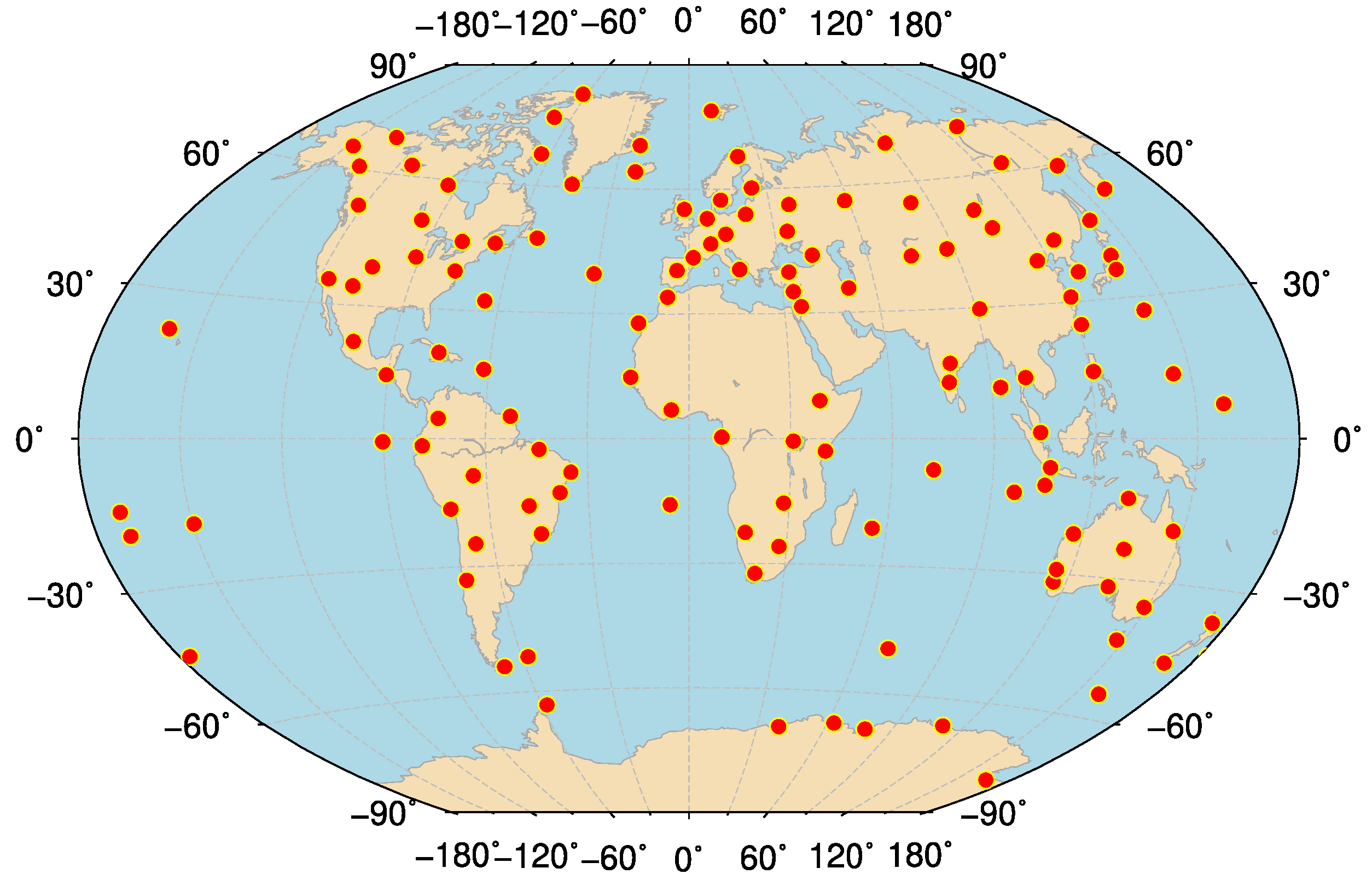
3.1. Data Collection and Processing Strategies

Data from 132 IGS stations observed during days 1 to 32 in 2018 are used in the experimental validation. Figure 3 shows the station distribution of the selected 132 IGS sites in global scale. We modified and applied the Positioning and Navigation Data Analysis (PANDA) software developed at Wuhan University in China to process the GPS data [30,31]. The detailed processing strategies are shown in Table 1, and the estimated parameters are the station coordinates, hourly zenith troposphere delays, 48 h troposphere gradients, receiver clock corrections for each epoch, and ambiguity in each arc.

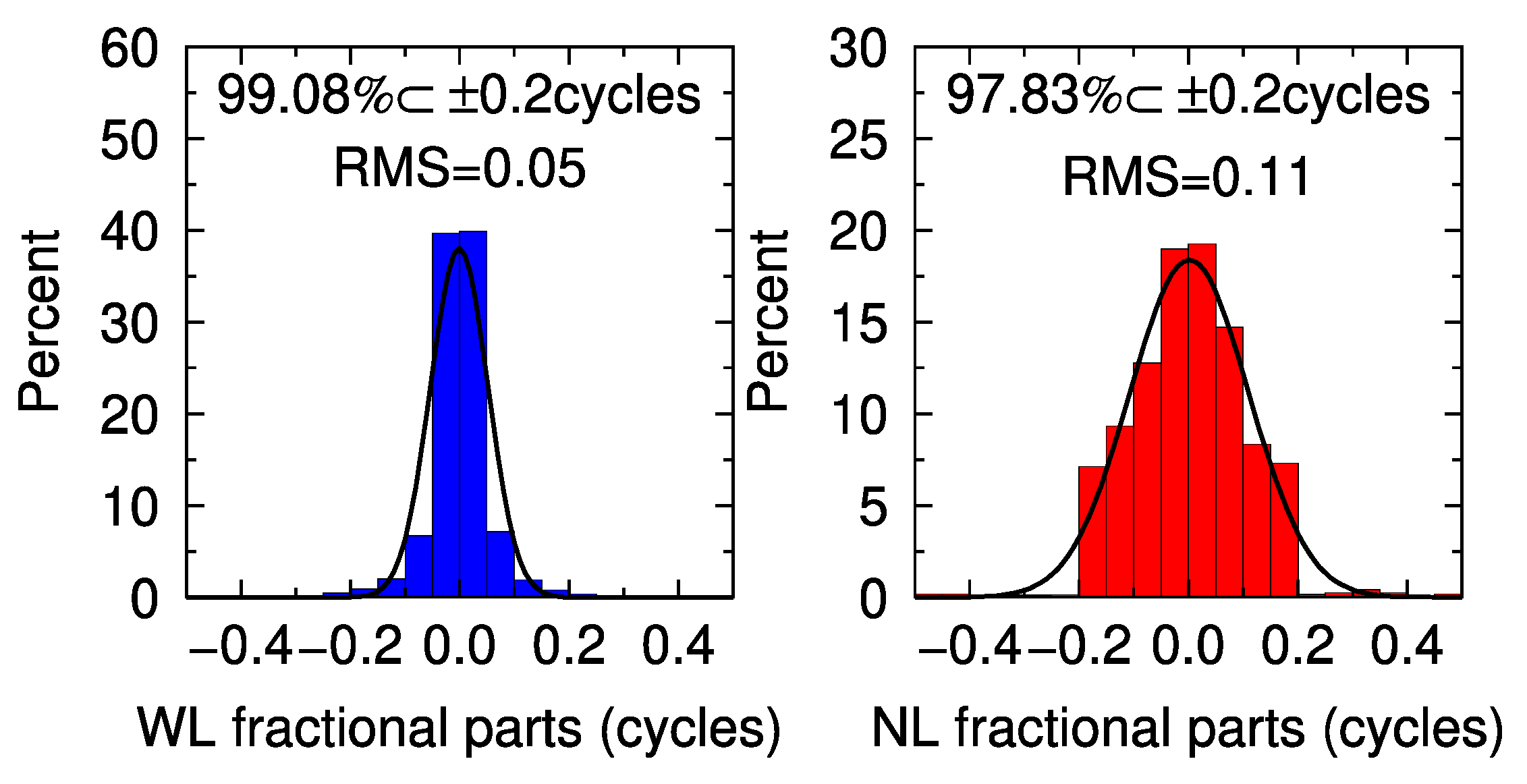
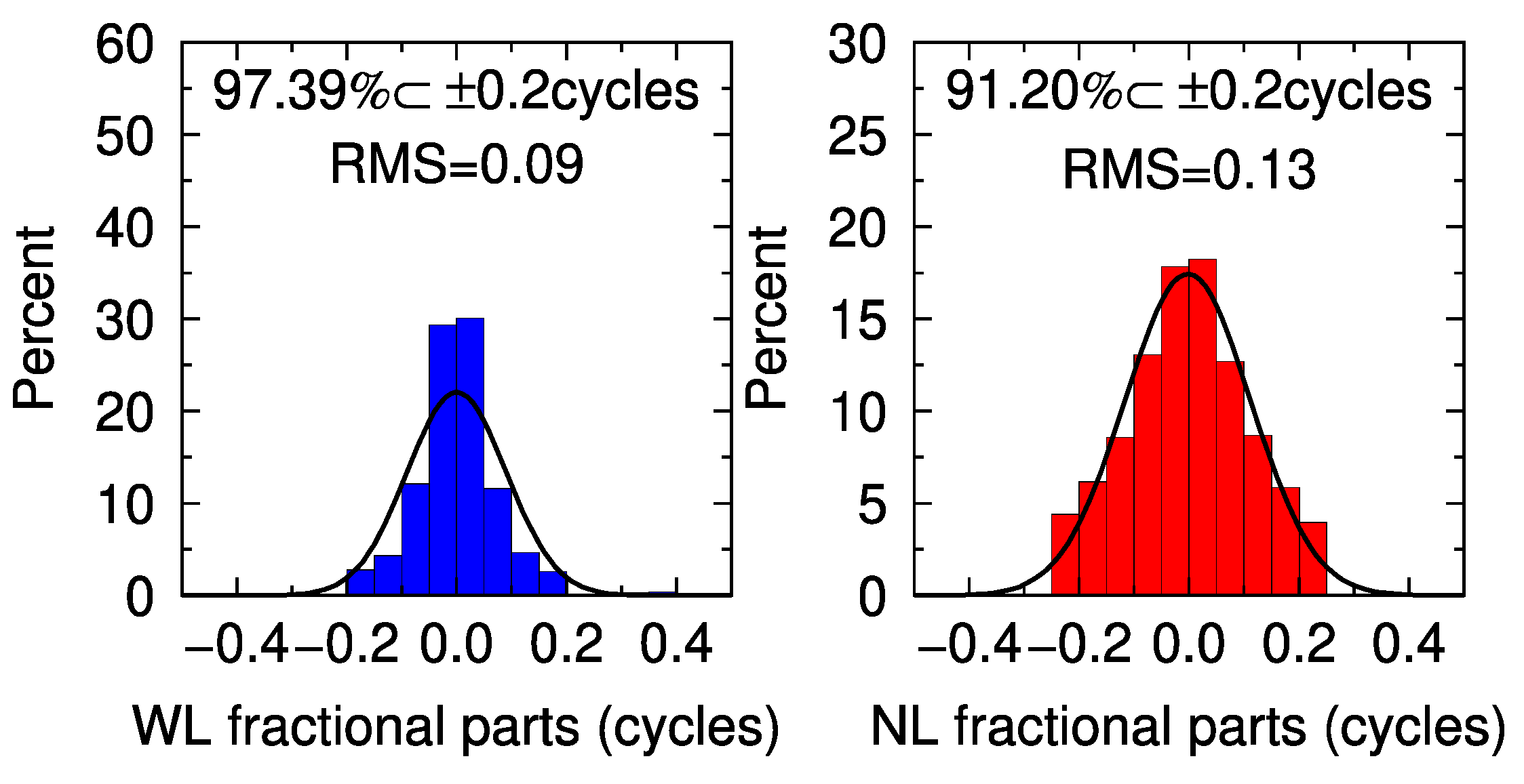
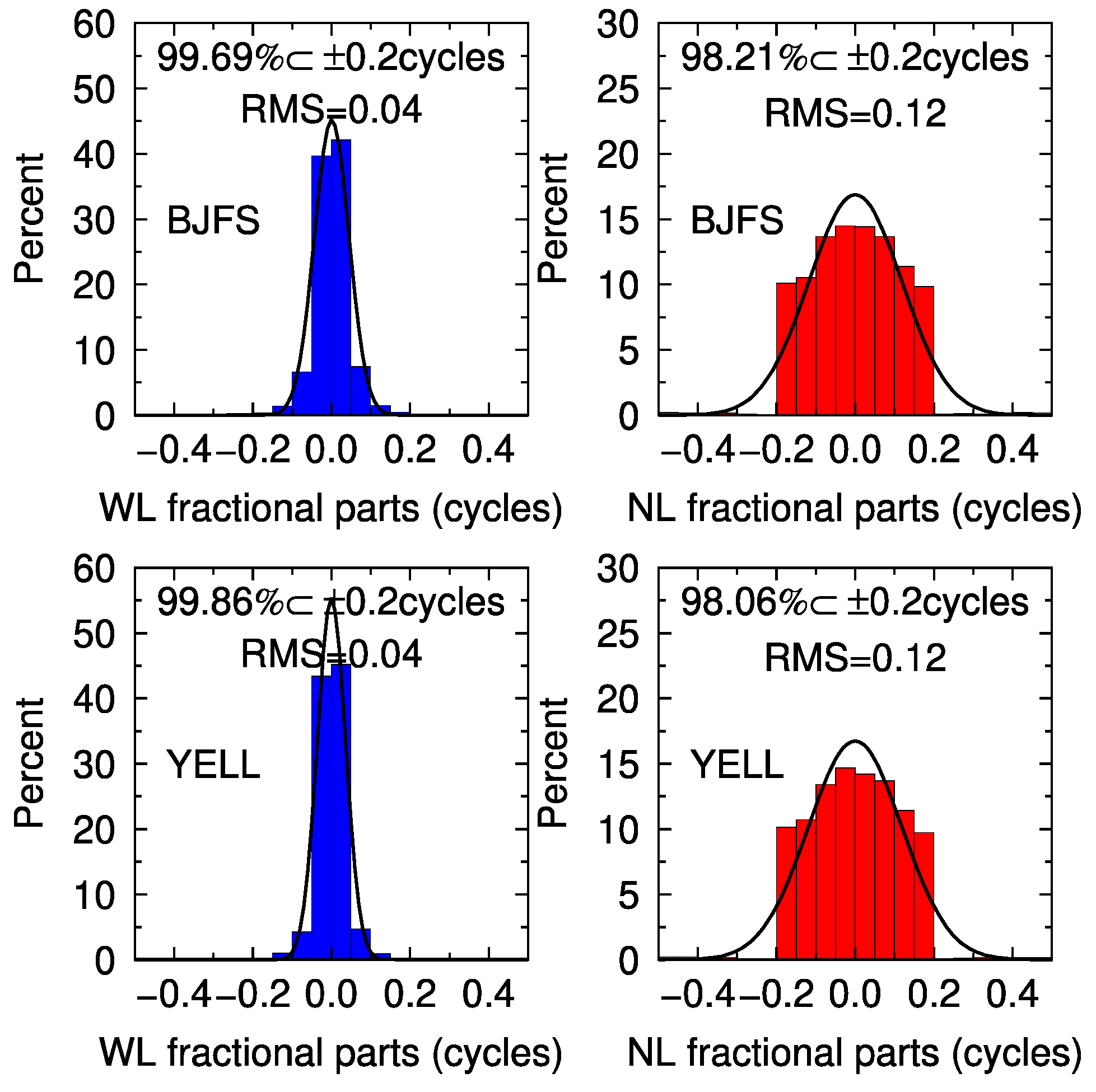
3.2. Fractional Parts of DD WL and NL Ambiguities

As previously mentioned, if the receiver and satellite related hardware delays could be removed, the DD WL and NL ambiguities should be recovered to the integer nature value. Therefore, the fractional parts of the DD WL and NL ambiguities are firstly assessed to analyze the performance of GPS ambiguity resolution. Figure 4 shows the fractional parts of the independent DD WL and NL ambiguities of all the stations on DOY 002-003 for the pass-by-pass ambiguity resolution in PPP (PPP). It demonstrates that 99.08% WL and 97.83% NL ambiguities are close to an integer within 0.2 cycles. To compare with the traditional DD network ambiguity resolution method, we applied the PANDA software to solve the network observations to obtain the network solution as well (NET). The corresponding distribution of the fractional parts of all the WL and NL ambiguities are shown in Figure 5. Only 97.39% and 91.20% of WL and NL ambiguities are close to integer. For the root mean squares (RMS) of the fractional parts, the proposed method is also lower than the NET method.
Then, we processed the data of BJFS and YELL in the whole year of 2018 and gave the statistics of the fractional parts of independent WL and NL ambiguities, as shown in Figure 6. Nearly 100% WL ambiguities are close to an integer within 0.2 cycles, and more than 98% of NL ambiguities within 0.2 cycles. Meanwhile, the fractional parts of all the ambiguities from Figure 4 to Figure 5 are satisfied the normal distribution.
From the previous analysis, we know that the hardware biases could be canceled to a large extent by differencing ambiguity candidates between satellites and two adjacent days. Therefore, DD ambiguities can be fixed to integers for a single GPS receiver.

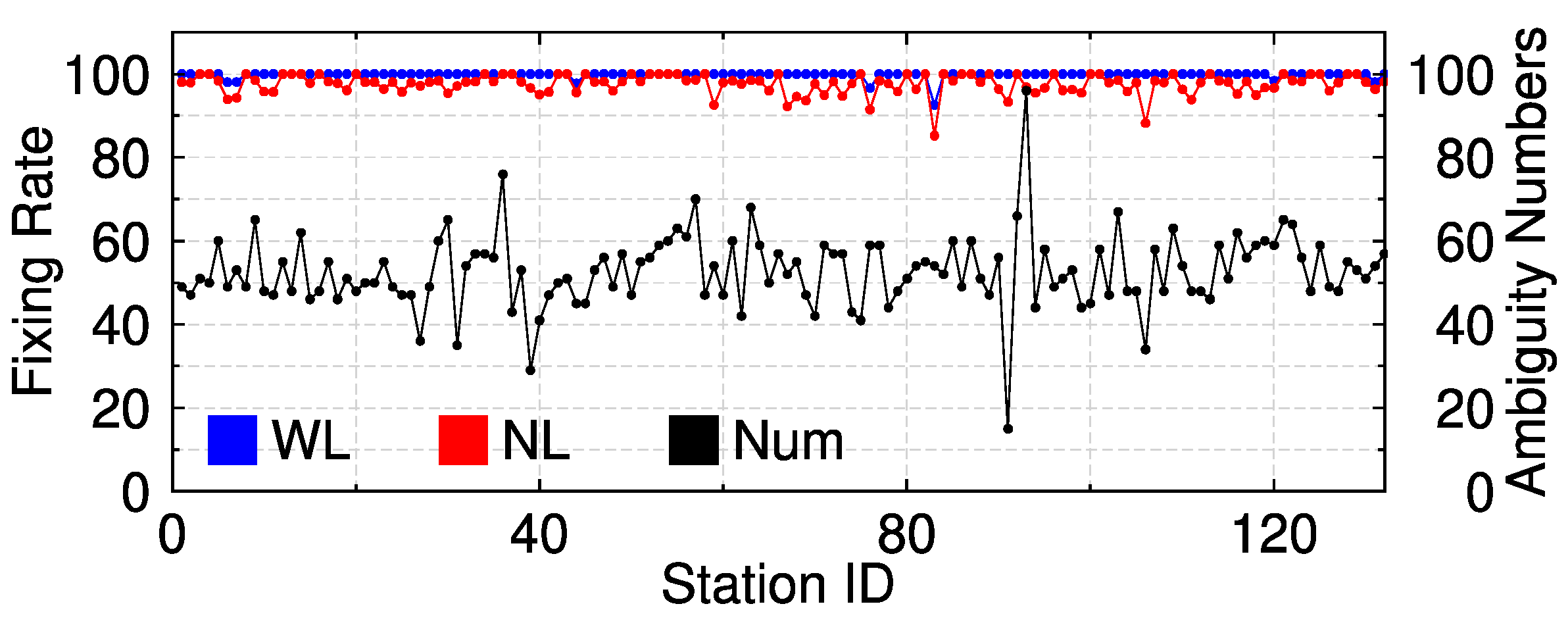
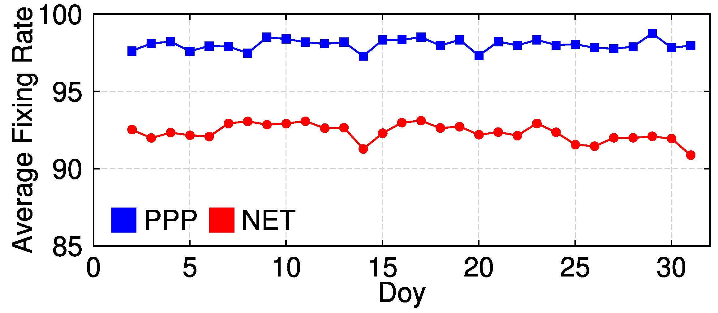
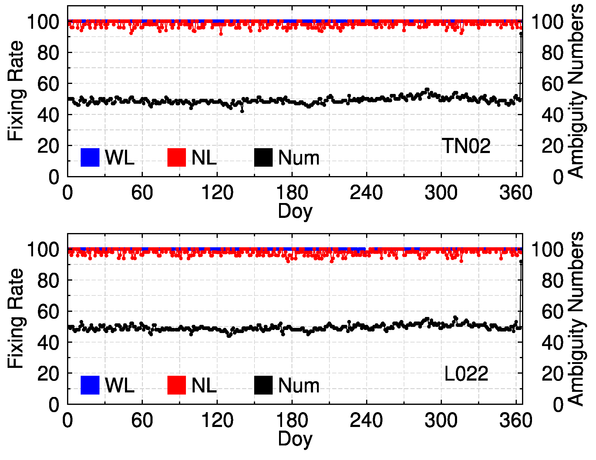
3.3. Ambiguity Fixing Rate

To assess the performance of the ambiguity fixing, we calculated the ambiguity fixing rate after processing GPS data of IGS network with the PPP method. Figure 7 shows the WL and NL ambiguity fixing rate statistics of the PPP for each station on DOY 002. Generally, there are 50 ambiguities for a station on average, and the WL ambiguity fixing rates of nearly all of stations are 100%, while the NL ambiguity fixing rates are mostly higher than 90%.
Figure 8 shows the mean averages of ambiguity fixing rate of all stations and baselines on each day with single receiver PPP and network solution. It clearly shows that the ambiguity fixing rate ranges between 97% to 98% for the single receiver PPP method, which is better than the network solution, with the latter ranging between 90% to 93%. This might be the result of the removal of the multipath effect in ambiguity estimates by differencing the observations between adjacent days. This confirms the feasibility of ambiguity resolution method by differencing the SD ambiguities parameters for the same satellite pair between two adjacent days.

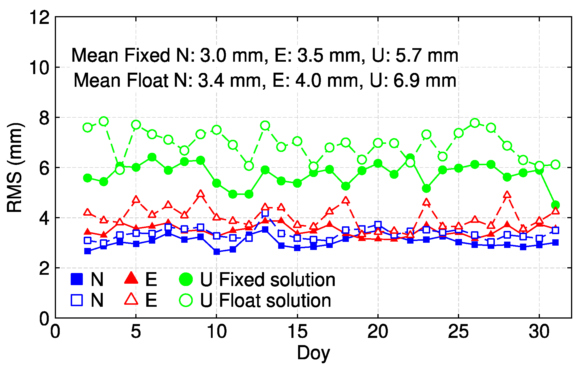
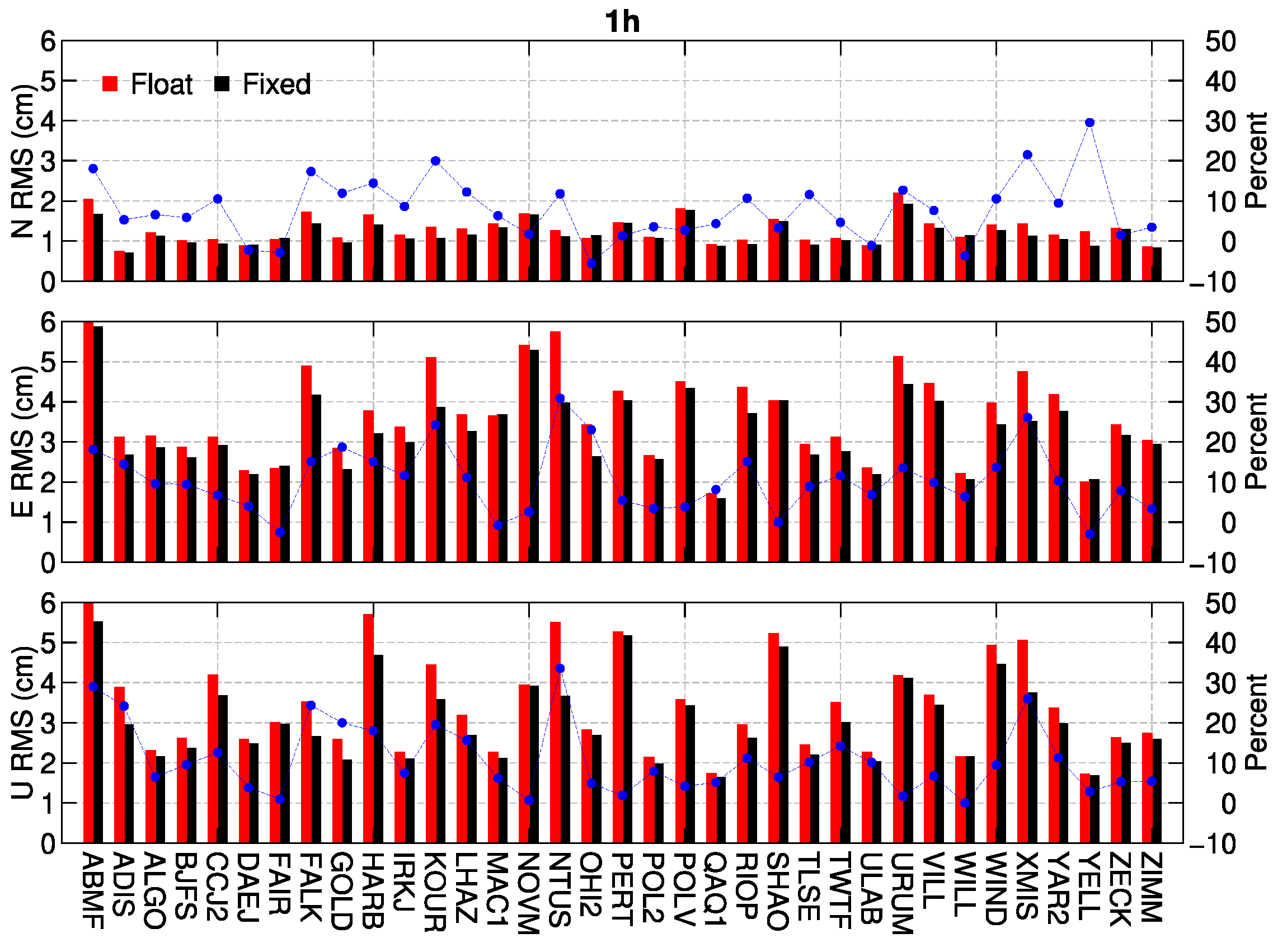
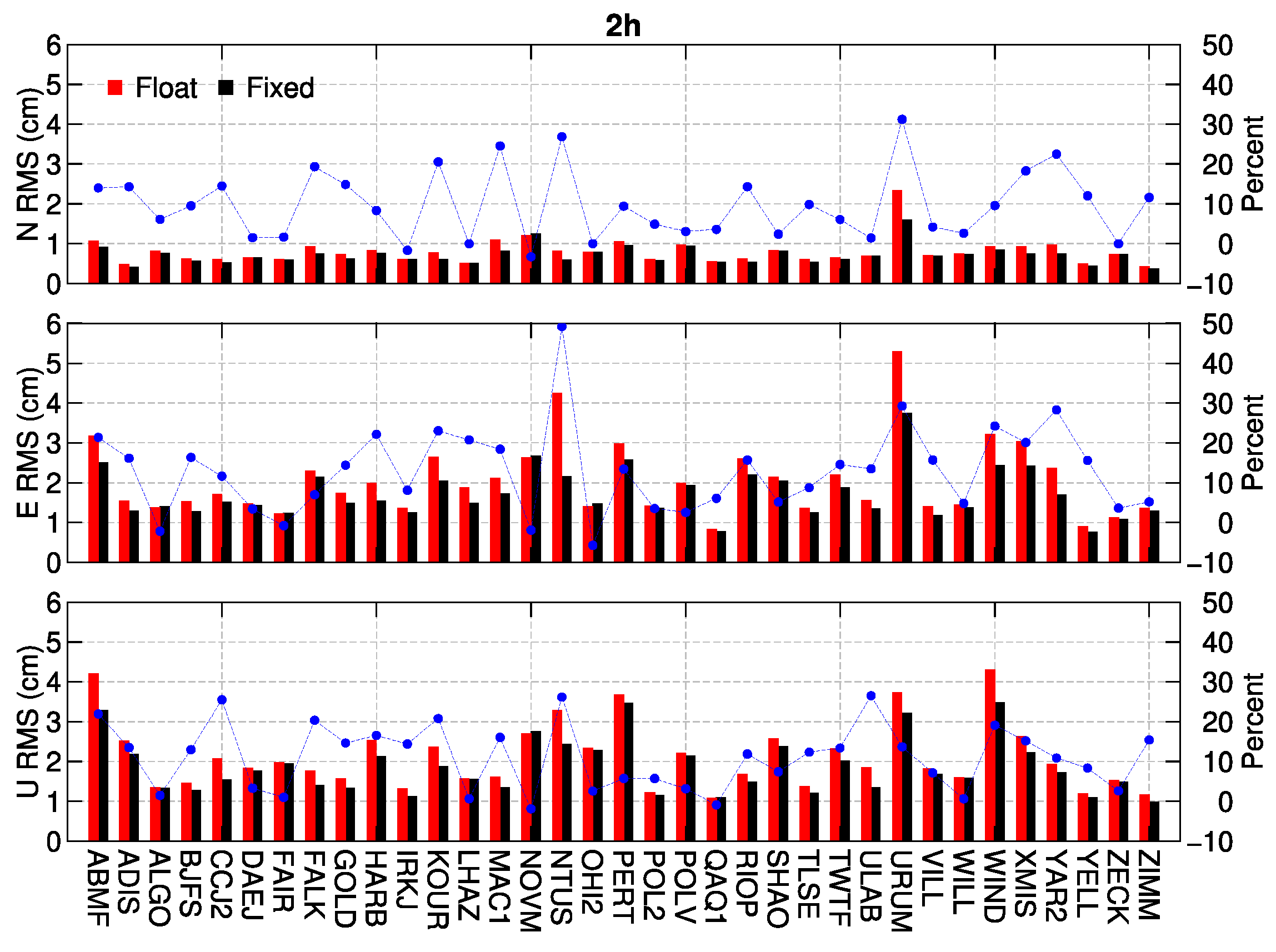
3.4. Positioning Accuracy Assessment

To demonstrate the performance of positioning, the estimated station coordinates with fixed and float ambiguities are compared with those of the IGS weekly solutions, respectively. A seven-parameter Helmert transformation was firstly applied to eliminate the possible systematic differences, then the averaged RMS in East, North and Up directions on each day are shown in Figure 9 [35]. It is observed that RMS of the fixed solutions in East and North directions vary between 2 to 4 mm, while for the Up direction the variance is about 6 mm, which is similar to the inconsistency between the Analysis Center’s and IGS final products. The float solutions are slightly lower than the fixed ones, with 3–5 mm in the horizontal component and 6–8 mm in the up direction. The mean position RMS is improved from (3.4 mm, 4.0 mm, and 6.9 mm) to (3.0 mm, 3.5 mm, and 5.7 mm) in north, east, and up directions, with an improvement of 13.3%, 12.5% and 17.4%, respectively.
To show the performance of ambiguity resolution in PPP with a short data length, we selected 35 stations randomly from the 132 IGS stations to conduct 1 h/2 h hourly PPP for a week from Doy 007 to 013 in 2018. Hence, there are 168 and 84 1 h and 2 h hourly solutions for a station with no data loss. Figure 10 and Figure 11 show the RMS of 1 h/2 h hourly positioning solutions with respect to the IGS weekly solutions. The RMSs of 1 h solutions are mostly better than 2 cm in the North direction, and 2–6 cm in East and Up directions, while the 2 h solutions are better than 1 h ones, with mostly 1 cm in the North, and 2cm in East and Up directions. The blue dots shown in the figures are the accuracy improvements of ambiguity fixed solutions compared with the float ones for each station. Roughly speaking, the accuracy of most stations is improved after fixing ambiguities; however, the improvements are limited for some stations, with less than 10%. In addition, Table 2 shows the mean positioning RMSs and mean percentage of accuracy improvement with the fixed ambiguities for the 35 stations. It shows that the mean position RMSs in the float and fixed 1 h hourly solutions are basically 1 cm in the North, and 3 cm in East and Up directions, while they are better than 1 cm in the North and 2 cm in East and Up directions for the 2 h hourly solutions. However, the percentages of accuracy improvements are roughly 10% after ambiguity resolution for 1 h/2 h hourly solutions.
The accuracy improvement of daily solutions after ambiguity resolution is 10%, which is consistent with the results of Ge et al. [8]. Geng et al. demonstrated that this is because of the float daily PPP solutions already achieving to millimeter accuracy level [16]. However, for hourly solutions, the pass-by-pass ambiguity resolution constraint is limited in accuracy improvement. This might be because of the positioning accuracy is mainly dependent on the satellite geometry transformation during the observation period. Thus, the accuracy improvements for the 2 h hourly solutions are slightly better than those of the 1 h hourly solutions.

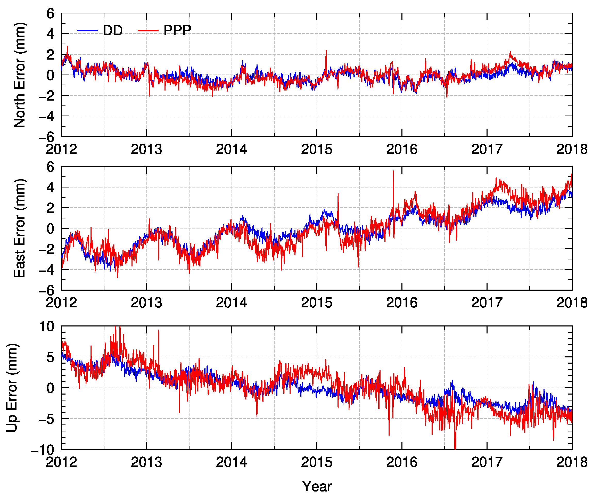
3.5. Deformation Monitoring Application

In order to assess the real-life positioning performance of the single receiver PPP with pass-by-pass ambiguity resolution, we applied a group of GPS data from a dam deformation monitoring system to carry out the experiment, where TN02 is the reference station and L022 is the monitoring station on the main dam. The observation period is from 2012 to 2018. Both of the stations are equipped with a TRIMBLE NETRS receiver and a CHOKE RING (TRM29659.00) antenna. The sampling rate is 30s. Figure 12 shows the ambiguity fixing rate of TN02 and L022 on each day for the whole year of 2013. As shown, the fixing rates of WL ambiguity are close to 100% and those of NL are higher than 90% for the two stations. The ambiguity number is around 50 for each day, which is similar to the IGS stations.
We processed the GPS observations of TN02 and L022 with PPP method and DD method by forming a baseline L022-TN02. Since the baseline length is less than 600 m, the precision of DD baseline solutions can reach up to 1 mm in horizonal component and 1–2 mm in vertical component. To generate the corresponding baseline solutions for PPP, we simply differenced the PPP solutions of TN02 and L022 and transmitted the baseline time series into NEU (Figure 13).
Figure 13 shows that the time series generated by PPP are in agreement with the DD baseline solutions, especially for the horizontal components. The annual movements and long-term trend can clearly be observed from the baseline time series. However, the PPP solutions show a larger noise compared with the DD solution, mainly in the high-frequency component of the time-series which might be the result of the large noise of IF combinations used by the PPP method.

4. Conclusions

In traditional precise point positioning applications, the phase ambiguities have to be kept as float parameters, due to the existence of receiver and satellite related hardware delays. To obtain the ambiguity-fixed solutions, a network of reference stations is required to form DD ambiguities, or the hardware delays are calibrated in advance and applied to single-receiver positioning models. In this study, we carried out an exploratory research of pass-by-pass ambiguity resolution method by differencing the satellite-related hardware delays between undifferenced ambiguity candidates in adjacent passes for two adjacent sidereal days and the receiver-related hardware delays between satellites for a single GPS receiver. Thus, ambiguity-fixed PPP solutions for a single receiver can be obtained without forming baselines and applying FCB corrections.
The pass-by-pass ambiguity resolution strategy is tested based on the GPS observations from 132 globally distributed stations of IGS during DOY 002-031, 2018. The results show that, 99.08% WL and 97.83% NL ambiguities for PPP method are close to an integer within 0.2 cycles, which are higher than the network solution with multiple receivers with 97.39% and 91.20%. On average, the ambiguity fixing rate of each day from DOY 002-031 is about 97% to 98% for the single receiver PPP, which is also higher than the network solutions with 90% to 93%. The estimated daily and hourly station coordinates are compared with that of the IGS weekly solutions. The RMSs in east and north directions are 2–4 mm and is about 6 mm in up directions for the fixed daily solutions, and 1–2 cm in north, and 2–3 cm in east and up directions for the fixed hourly solutions. The accuracy of daily and hourly solutions can be improved by roughly 10% after ambiguity resolution. Finally, we applied a group of data from a dam deformation monitoring system to validate the performance of pass-by-pass ambiguity resolution in real-life applications. It shows that the fixing rate of WL ambiguity is close to 100% and of NL is higher than 90% for the two stations, and the time series generated by PPP are in agreement with the DD baseline solutions.
With the pass-by-pass ambiguity resolution method, the single receiver ambiguity-fixed solutions can be obtained without applying the external FCB corrections. However, the current method is only applicable for the static post precise point positioning. The research of ambiguity resolution in kinematic solution and real-time mode with a single receiver is still needed to be carried out in the future.

Author Contributions

Conceptualization, W.J., P.P., X.M. and C.X.; methodology, R.X., Q.C. and P.P.; software, R.X. and P.P.; validation, R.X. and P.P.; formal analysis, X.M.; investigation, P.P.; resources, C.X.; data curation, W.J. and Q.C.; writing—original draft preparation, R.X. and Q.C.; writing—review and editing, W.J., P.P., X.M. and C.X.; visualization, C.X.; supervision, P.P. and X.M.; project administration, W.J.; funding acquisition, W.J. and R.X. All authors have read and agreed to the published version of the manuscript.

Funding

This work was supported in part by the National key R&D Program of China under Grant 2018YFC1503601, the LIESMARS Special Research Funding and the National Dam Safety Research Center (Grant No. CX2019B05). This research was also supported by the National Natural Science Foundation of China (Grant No. 41525014 and 42004017) and the National Science Innovation Group Foundation of China (Grant No. 41721003). Thank goes to The Office of China Postdoctoral Council for providing the first author a scholarship which allows him to visit the University of Nottingham for two years to research in the UK from October 2019 (No: 20190050).

Data Availability Statement

The GPS data, IGS final precise orbit and clock products can be found from the website of IGS data center of Wuhan University via ftp://igs.gnsswhu.cn/pub/gnss/ (accessed on 20 August 2021).

Conflicts of Interest

The authors declare no conflict of interest.

References

  1. Psimoulis, P.A.; Houlie, N.; Habboub, M.; Michel, C.; Rothacher, M. Detection of ground motions using high-rate GPS time-series. Geophys. J. Int. 2018, 214, 1237–1251. [Google Scholar] [CrossRef] [Green Version]
  2. Newman, A.V.; Stiros, S.; Feng, L.; Psimoulis, P.; Vamvakaris, D. Recent geodetic unrest at Santorini Caldera, Greece. Geophys. Res. Lett. 2012, 39, L06309. [Google Scholar] [CrossRef]
  3. Hudnut, K.W.; Behr, J.A. Continuous GPS Monitoring of Structural Deformation at Pacoima Dam, California. Seismol. Res. Lett. 1998, 69, 299–308. [Google Scholar] [CrossRef]
  4. Meng, X.; Nguyen, D.T.; Xie, Y.; Owen, J.S.; Psimoulis, P.; Ince, S.; Chen, Q.; Ye, J.; Bhatia, P. Design and Implementation of a New System for Large Bridge Monitoring—GeoSHM. Sensors 2018, 18, 775. [Google Scholar] [CrossRef] [PubMed] [Green Version]
  5. Psimoulis, P.; Ghilardi, M.; Fouache, E.; Stiros, S. Subsidence and evolution of the Thessaloniki plain, Greece, based on historical leveling and GPS data. Eng. Geol. 2007, 90, 55–70. [Google Scholar] [CrossRef]
  6. Ge, M.; Gendt, G.; Dick, G.; Zhang, F.P. Improving carrier-phase ambiguity resolution in global GPS network solutions. J. Geod. 2005, 79, 103–110. [Google Scholar] [CrossRef]
  7. Ge, M.; Gendt, G.; Dick, G.; Zhang, F.P.; Rothacher, M. A new data processing strategy for huge GNSS global networks. J. Geod. 2006, 80, 199–203. [Google Scholar] [CrossRef]
  8. Ge, M.; Gendt, G.; Rothacher, M.A.; Shi, C.; Liu, J. Resolution of GPS carrier-phase ambiguities in precise point positioning (PPP) with daily observations. J. Geod. 2008, 82, 389–399. [Google Scholar] [CrossRef]
  9. Khodabandeh, A.; Teunissen, P. Integer estimability in GNSS networks. J. Geod. 2019, 93, 1805–1819. [Google Scholar] [CrossRef] [Green Version]
  10. Teunissen, P.; Khodabandeh, A. Review and principles of PPP-RTK methods. J. Geod. 2015, 89, 217–240. [Google Scholar] [CrossRef]
  11. King, M.; Colemar, R.; Nguyen, L.N. Spurious periodic horizontal signals in sub-daily GPS position estimates. J. Geod. 2003, 77, 15–21. [Google Scholar] [CrossRef]
  12. Tregoning, P.; Watson, C. Atmospheric effects and spurious signals in GPS analyses. J. Geophys. Res. Solid Earth 2009, 114, B09403. [Google Scholar] [CrossRef] [Green Version]
  13. Khodabandeh, A. Single-station PPP-RTK: Correction latency and ambiguity resolution performance. J. Geod. 2021, 95, 42–66. [Google Scholar] [CrossRef]
  14. Laurichesse, D.; Mercier, F.; Berthias, J.P.; Broca, P.; Cerri, L. Integer Ambiguity Resolution on Undifferenced GPS Phase Measurements and Its Application to PPP and Satellite Precise Orbit Determination. Navigation 2009, 56, 135–149. [Google Scholar] [CrossRef]
  15. Collins, P. Isolating and estimating undifferenced GPS integer ambiguities. In Proceedings of the ION National Technical Meeting, San Diego, CA, USA, 28–30 January 2008; pp. 720–732. [Google Scholar]
  16. Geng, J.; Meng, X.; Dodson, A.H.; Teferle, F.N. Integer ambiguity resolution in precise point positioning: Method comparison. J. Geod. 2010, 84, 569–581. [Google Scholar] [CrossRef] [Green Version]
  17. Shi, J.; Gao, Y. A comparison of three PPP integer ambiguity resolution methods. GPS Solut. 2014, 18, 519–528. [Google Scholar] [CrossRef]
  18. Montenbruck, O.; Hackel, S.; Ijssel, J.; Arnold, D. Reduced dynamic and kinematic precise orbit determination for the Swarm mission from 4 years of GPS tracking. GPS Solut. 2018, 22, 79. [Google Scholar] [CrossRef]
  19. Zhou, X.; Chen, H.; Fan, W.; Zhou, X.; Chen, Q.; Jiang, W. Assessment of single-difference and track-to-track ambiguity resolution in LEO precise orbit determination. GPS Solut. 2021, 25, 1–15. [Google Scholar] [CrossRef]
  20. Montenbruck, O.; Hackel, S.; Jaggi, A. Precise orbit determination of the Sentinel-3A altimetry satellite using ambiguity-fixed GPS carrier phase observations. J. Geod. 2018, 92, 711–726. [Google Scholar] [CrossRef] [Green Version]
  21. An, X.; Meng, X.; Chen, H.; Jiang, W.; Xi, R.; Chen, Q. Combined precise orbit determination of GPS and GLONASS with ambiguity resolution. J. Geod. 2019, 93, 2585–2603. [Google Scholar] [CrossRef]
  22. Saastamoinen, J. Atmospheric correction for the troposphere and stratosphere in radio ranging satellites. Use Artif. Satell. Geod. 1972, 15, 247–251. [Google Scholar]
  23. Hatch, R. The synergism of GPS code and carrier measurements. In Proceedings of the Third International Symposium on Satellite Doppler Positioning, Las Cruces, NM, USA, 8–12 February 1982; Volume 2, pp. 1213–1231. [Google Scholar]
  24. Melbourne, W.G. The case for ranging in GPS-based geodetic systems. In Proceedings of the First International Symposium on Precise Positioning with the Global Positioning System, Rockville, MD, USA, 15–19 April 1985. [Google Scholar]
  25. Wübbena, G. Software developments for geodetic positioning with GPS using TI-4100 code and carrier measurements. In Proceedings of the First International Symposium on Precise Positioning with the Global Positioning System, Rockville, MD, USA, 15–19 April 1985. [Google Scholar]
  26. Dong, D.; Bock, Y. Global Positioning System network analysis with phase ambiguity resolution applied to crustal deformation studies in California. J. Geophys. Res. Solid Earth 1989, 94, 3949–3966. [Google Scholar] [CrossRef]
  27. Blewitt, G. An Automatic Editing Algorithm for GPS data. Geophys. Res. Lett. 1990, 17, 199–202. [Google Scholar] [CrossRef] [Green Version]
  28. Agnew, D.C.; Larson, K.M. Finding the repeat times of the GPS constellation. GPS Solut. 2007, 11, 71–76. [Google Scholar] [CrossRef]
  29. Larson, K.M.; Bilich, A.; Axelrad, P. Improving the precision of high-rate GPS. J. Geophys. Res. 2007, 112, B05422. [Google Scholar] [CrossRef]
  30. Liu, J.; Ge, M. PANDA software and its preliminary result of positioning and orbit determination. Wuhan Univ. J. Nat. Sci. 2003, 8, 603–609. [Google Scholar]
  31. Shi, C.; Zhao, Q.; Geng, J.; Lou, Y.; Liu, J. Recent development of PANDA software in GNSS data processing. In Proceedings of the SPIE 7285, International Conference on Earth Observation Data Processing and Analysis (ICEODPA), Wuhan, China, 28–30 December 2008. [Google Scholar]
  32. Boehm, J.; Niell, A.; Tregoning, P.; Schuh, H. Global mapping function (GMF): A new empirical mapping function based on numerical weather model data. Geophys. Res. Lett. 2006, 33, L07304. [Google Scholar] [CrossRef] [Green Version]
  33. Chen, G.; Herring, T.A. Effects of atmospheric azimuthal asymmetry on the analysis of space geodetic data. J. Geophys. Res. 1997, 102, 20489–20502. [Google Scholar] [CrossRef]
  34. Lyard, F.; Lefevre, F.; Letellier, T.; Francis, O. Modelling the global ocean tides: Modern insights from FES2004. Ocean Dyn. 2006, 56, 394–415. [Google Scholar] [CrossRef]
  35. Chen, H.; Jiang, W.; Ge, M.; Wickert, J.; Schuh, H. An enhanced strategy for GNSS data processing of massive networks. J. Geod. 2014, 88, 857–867. [Google Scholar] [CrossRef]
Figure 1. The diagram of forming DD WL ambiguity.
Remotesensing 13 03728 g001
Figure 2. Flowchart of data processing.
Remotesensing 13 03728 g002
Figure 3. Station distribution.
Remotesensing 13 03728 g003
Figure 4. Distribution of the fractional parts of all the WL and NL ambiguities for the PPP method on DOY 002-003.
Remotesensing 13 03728 g004
Figure 5. Distribution of the fractional parts of all the WL and NL ambiguities for network resolution on DOY 002.
Remotesensing 13 03728 g005
Figure 6. Distribution of the fractional parts of all the WL and NL ambiguities for BJFS and YELL on the whole year of 2018.
Remotesensing 13 03728 g006
Figure 7. Ambiguity fixing rate and ambiguity numbers of IGS stations on DOY 002 with PPP method.
Remotesensing 13 03728 g007
Figure 8. Means of ambiguity fixing rate of all stations.
Remotesensing 13 03728 g008
Figure 9. Averaged RMS statistics in east, north and up directions on each day during the experimental period.
Remotesensing 13 03728 g009
Figure 10. RMS of the float and fixed position estimates for 1 h hourly data length with respect to the weekly estimates for 35 stations during 7days.
Remotesensing 13 03728 g010
Figure 11. RMS of the float and fixed position estimates for 2 h hourly data length with respect to the weekly estimates for 35 stations during 7days.
Remotesensing 13 03728 g011
Figure 12. The ambiguity fixing rate of TN02 and L022 on each day for the whole year of 2013.
Remotesensing 13 03728 g012
Figure 13. Time series comparison between PPP solutions and DD baseline resolutions.
Remotesensing 13 03728 g013
Table 1. PPP data processing strategies.
ItemsStrategies
ObservationsUndifferenced IF combination of code and phase observations
Parameter estimationLeast squares
Reference FrameITRF2014
Cut-off elevation
Sampling rate30s
Session length48h
Weight methodElevation dependent weighting method
Phase Center OffsetPCO/PCV corrections, igs14_2045.atx
Phase wind-upCorrected
Tropospheric delaysMapping function: GMF [32]; Zenith delay parameters for station with a 1 h interval; 48 h gradients for north and east horizontal delays [33]
Receiver clocksSolved at each epoch (white noise process)
Tidal CorrectionsFES2004 [34]
Table 2. Mean position RMS in the float and fixed 1 h/2 h hourly solutions, and the accuracy improvements after fixing the ambiguities for the 35 stations.
Session LengthFloat Solutions (cm)Fixed Solutions (cm)Improvement
NEUNEUNEU
1 h1.33.73.51.23.23.18.4%11.4%12.4%
2 h0.82.02.10.71.71.810.8%15.8%11.8%
Publisher’s Note: MDPI stays neutral with regard to jurisdictional claims in published maps and institutional affiliations.

