Article

Modal Parameters Identification of Bridge Structures from GNSS Data Using the Improved Empirical Wavelet Transform

1
Key Laboratory for Wind and Bridge Engineering of Hunan Province, Hunan University, Changsha 410082, China
2
College of Architecture and Civil Engineering, Beijing University of Technology, Beijing 100124, China
*
Author to whom correspondence should be addressed.
Remote Sens. 2021, 13(17), 3375; https://doi.org/10.3390/rs13173375
Submission received: 9 July 2021 / Revised: 19 August 2021 / Accepted: 23 August 2021 / Published: 25 August 2021

Abstract

:
It is difficult to accurately identify the dynamic deformation of bridges from Global Navigation Satellite System (GNSS) due to the influence of the multipath effect and random errors, etc. To solve this problem, an improved empirical wavelet transform (EWT)-based procedure was proposed to denoise GNSS data and identify the modal parameters of bridge structures. Firstly, the Yule–Walker algorithm-based auto-power spectrum and Fourier spectrum were jointly adopted to segment the frequency bands of structural dynamic response data. Secondly, the improved EWT algorithm was used to decompose and reconstruct the dynamic response data according to a correlation coefficient-based criterion. Finally, Natural Excitation Technique (NExT) and Hilbert Transform (HT) were applied to identify the modal parameters of structures from the decomposed efficient components. Two groups of simulation data were used to validate the feasibility and reliability of the proposed method, which consisted of the vibration responses of a four-storey steel frame model, and the acceleration response data of a suspension bridge. Moreover, field experiments were carried out on the Wilford suspension bridge in Nottingham, UK, with GNSS and an accelerometer. The fundamental frequency (1.6707 Hz), the damping ratio (0.82%), as well as the maximum dynamic displacements (10.10 mm) of the Wilford suspension bridge were detected by using this proposed method from the GNSS measurements, which were consistent with the accelerometer results. In conclusion, the analysis revealed that the improved EWT-based method was capable of accurately identifying the low-order, closely spaced modal parameters of bridge structures under operational conditions.

1. Introduction

Global Navigation Satellite System (GNSS) positioning technology, as an innovative monitoring method, features the provision of real-time 3D absolute displacements of monitoring structures; continuously autonomous operation, regardless of the weather and visibility conditions; and easy operation. Additionally, the GNSS positioning technology can overcome some shortcomings of traditional monitoring methods, as it easily identifies low-frequency structural vibration responses. It has been widely used in the bridge deformation monitoring in the last few years [1,2,3,4]. However, due to the existence of the multipath effect and random errors, true dynamic displacements are often overflooded by strong noise, which limits the GNSS vibration monitoring in modal parameters identification [5,6]. Hence, data processing methods should be used to eliminate GNSS measurement error before extracting the structural dynamic characteristics.
The data processing methods consist of the time domain methods, the frequency domain methods, and the time–frequency domain methods [7]. Bridge vibration responses are usually nonlinear and non-stationary, and the local time-varying characteristic may be ignored by using methods with a single parameter of time or frequency [8]. Consequently, time–frequency methods, which can provide instantaneous data information in both time and frequency domains, are becoming more competitive to process structural health monitoring (SHM) data [9]. In recent years, some time–frequency domain methods have been widely used in the identification of structural and modal parameters, and have shown a good performance. Time–frequency domain methods are mainly divided into two groups. One group is wavelet transform (WT) and its variants, such as continuous wavelet transform (CWT), least-squares wavelet analysis (LSWA), and weighted wavelet analysis (WWA). The other group includes empirical mode decomposition (EMD), ensemble empirical mode decomposition (EEMD) and multivariate empirical mode decomposition (MEMD), etc. [10,11,12,13,14].
In terms of noise reduction, data processing methods based on WT and EMD have been widely studied. WT can provide a high time–frequency resolution, by selecting a suitable basis function and a decomposition scale. However, the non-adaptive binary frequency partition technique may cause modal aliasing and false modes. Huang et al. [15] proposed empirical mode decomposition (EMD), a well-known adaptive approach, to adaptively decompose the oscillatory data into sets of Intrinsic Mode Functions (IMFs). This method was able to separate stationary and non-stationary components effectively. However, the major shortcomings of the EMD are a lack of mathematical theory, mode aliasing, and the end effect [16].
A novel empirical wavelet transform (EWT) has been developed recently by Gilles [17,18], combining the advantages of WT and EMD. The main idea of EWT is to determine the segmentation of spectrum and then build a wavelet filter bank to decompose the vibration responses into a series of IMFs. Furthermore, the modal parameters are derived from the EWT-extracted IMFs by using Natural Excitation Technique (NExT) and Hilbert transform (HT). The EWT method exhibits calculation efficiency, excellent adaptation, and consolidated mathematic foundation. It is highly favorable for the processing and interpretation of non-stationary and complex data. Therefore, EWT demonstrates outstanding performance in various applications of machine fault diagnosis, seismic data analysis, image processing, medical disease diagnosis, and so on [19,20,21,22,23]. The vibration responses of engineering structures are usually complex due to the structural scale and intricate interactions between structures and dynamic loadings. There will be improper frequency band division and false modes when the EWT method is applied to the above structural health monitoring data.
Recently, several improvements or modifications have been proposed to overcome the shortcomings of traditional EWT. One way to improve the traditional EWT is employing a spectrum other than the Fourier, one which is used for an appropriate boundaries division, such as the pseudospectrum [24,25], power spectrum [26], scale–space representation [27], and time–frequency representation [28]. Amezquita-Sanchez et al. [24,25] presented a pseudospectrum segment method based on multiple signal classification (MUSIC). The MUSIC-EWT method identified the first six natural frequencies (NFs) and damping ratios (DRs) of the 123-storey Lotte World Tower. Xin et al. [26,28] used a standardized autoregression power spectrum calculated by the Burg algorithm and the time–frequency representation determined by Synchro-extracting Transform (SET) to define the boundaries for EWT analysis. The enhanced EWT methods reliably identified the loosely spaced modes of a real footbridge and the instantaneous frequencies of a time-varying highway bridge. Xia et al. [27] separated the mono-components from the health monitoring data of the civil structure via scale–space EWT and obtained the instantaneous modal parameters by the FREEVIB method. Another way to improve the traditional EWT is optimizing the Fourier spectrum segmentation method. Hu et al. [16] presented an enhanced EWT based on the envelope of the Fourier spectrum, calculated by the order statistic filter, and with criterions presented to pick out useful peaks. Dong et al. [29] proposed an EWT algorithm of modified spectrum separation based on the local window maxima (LWM) method. The experimental results indicated that the proposed method performed better than the original EWT method in identifying different damage mechanisms of composite structures. EWT achieved some successful applications in the field of the modal identification of civil structures, but the measurements were mainly based on the accelerometer whose data features were simpler and clearer than GNSS. Moreover, fewer studies discussed the judgment criterion of effective IMFs among a series of EWT-extracted IMFs. With the continuous development of GNSS hardware and software, it was crucial to identify the structural modes and dynamic displacements from GNSS vibration monitoring data.
In this paper, an improved EWT-based method is presented to denoise data and identify the modal parameters of bridge structures. Three steps are involved in the proposed method. Firstly, an auto-power spectrum based on the Yule–Walker algorithm [30] and the Fourier amplitude spectrum are jointly applied to build the appropriate boundaries. Secondly, the improved EWT algorithm is used to decompose the GNSS coordinate time series into a number of effective IMFs and reconstruct the dynamic response according to a correlation coefficient-based criterion. Thirdly, effective IMFs are further used to identify the structural modal parameters, NFs and DRs, by using Natural Excitation Technique (NExT) and Hilbert transform (HT). Numerical and experimental studies are conducted in this study to validate the feasibility and reliability of this proposed method.
The paper is organized as follows. In Section 2, the basic principles of the improved EWT algorithm and modal parameters identification based on the improved EWT are explained briefly, and the flowchart of data denoising and modal parameters identification is provided. Section 3 verifies the feasibility and accuracy of the improved EWT-based method for the identification of structural and modal parameters. Numerical studies on the vibration responses of a four-storey steel frame model, and acceleration response data of a suspension bridge are provided. In Section 4, field experiments with GNSS and an accelerometer on the Wilford pedestrian bridge located in Nottingham, UK, are conducted to further validate the capability of the proposed method. Finally, the conclusions are presented in Section 5.

2. Methodology

In order to further improve the identification accuracy of operational modal of bridge structures, this paper proposes an improved EWT-based method to denoise data and identify modal parameters, as shown in Figure 1. In the first step, the vibration responses data are collected from a real bridge by GNSS receivers. In the second step, the improved EWT method is applied for data denoising and dynamic displacements reconstruction. When the effective IMFs are defined by applying judgment criteria, NExT, HT and a nonlinear exponential function are subsequently performed to extract the modal information: NF and DR.

2.1. The Improved EWT

The traditional EWT process contains three important aspects [17]: (1) The data spectrum is segmented. First, the local maxima of the standardized Fourier spectrum are estimated, and the boundaries of various frequencies are defined as the center point between two consecutive maxima in Equation (1). (2) The empirical wavelets, which are equivalent to build a set of bandpass filters, are constructed. Centered around each boundary, a transition phase T n of width 2 τ n is defined for construction. The empirical scaling function and the empirical wavelets is defined by Equations (2) and (3), respectively. (3) The individual components or the approximate mono amplitude-modulation-frequency-modulation (AM-FM) components are extracted by applying the wavelet filter banks to divide the data into frequency sub-bands. The IMF S k is given in Equation (4):
ω n = { 0 , n = 0 Ω n + Ω n + 1 2 , n = 1 , 2 , , N 1 π n = N ,
where, ω n is the segmentation boundaries, and Ω n is the corresponding angular frequency of the local maxima:
ϕ n ( ω ) = { 1 , cos [ π 2 β ( 1 2 γ ω n + 1 ( | ω | ( 1 γ ) ω n + 1 ) ) ] 0 , , | ω | ( 1 γ ) ω n ( 1 γ ) ω n | ω | ( 1 + γ ) ω n otherwise ,
ψ ^ n ( ω ) = { 1 ,                  ( 1 + γ ) ω n | ω | ( 1 γ ) ω n + 1 cos [ π 2 β ( 1 2 γ ω n + 1 ( | ω | ( 1 γ ) ω n + 1 ) ) ] ,   ( 1 γ ) ω n + 1 | ω | ( 1 γ ) ω n + 1 sin [ π 2 β ( 1 2 γ ω n + 1 ( | ω | ( 1 γ ) ω n ) ) ] ,    ( 1 γ ) ω n | ω | ( 1 + γ ) ω n 0 ,                     otherwise ,
where, β ( x ) = x 4 ( 35 84 x + 70 x 2 20 x 3 ) , 0 < y < 1 and y < m i n n ( ω n + 1 ω n ω n + 1 + ω n ) .
s n ( t ) = { W s ε ( 0 , t ) · ϕ 1 ( t ) , n = 0 W s ε ( k , t ) · ψ k ( t ) , n = k ,
where, W s ε ( 0 , t ) is the detail coefficient, and W s ε ( k , t ) is the approximation coefficient.
The spectrum segmentation is at the core of EWT for adaptively obtaining ideal frequency bands. However, the Fourier spectrum is very sensitive to noise, leading to spurious local maxima. The traditional EWT segmentation method may lead to an improper separation when the data are contaminated with significant noise and/or nonstationary components. The autoregression power spectrum is smoothed with a lower-level variance and can define the boundaries more appropriately than the Fourier spectrum. Li et al. [30] studied three common algorithms of the power spectrum of the autoregression model. The Yule–Walker method had good resolution and met the requirement for analyzing the EEG data through comparative analysis. Under these circumstances, an auto-power spectrum based on the Yule–Walker algorithm and the Fourier spectrum are combined to define the appropriate boundaries in this study.
According to the theory of spectral analysis, stationary random data x ( n ) can be regarded as the output of a causal stable reversible system H ( z ) excited by Gaussian white noise. The output H ( z ) can be represented by a p-order Autoregressive (AR) model. It can be written as:
H ( z ) = G 1 + i = 1 p a i z i ,
where, a i and gain G are called predicted coefficients. Furthermore, the output x ( n ) can be expressed as:
x ( n ) = i = 1 p a i x ( n i ) + G ω ( n ) ,
where, ω n is the Gaussian white noise.
Based on the Yule–Walker algorithm, the regular equation of the AR model is obtained, and the auto-power spectral density estimation of the random data is calculated according to the solved p + 1 parameters. The auto-power spectrum can be defined as follows:
R x ( m ) = { i = 1 p a i R x ( i ) + G 2 ,      m = 0 i = 1 p a i R x ( m i ) , m = 1 , 2 , , p ,
P A R ( ω ) = G 2 | 1 + k = 1 p a k R x ( k ) + G 2 | ,
The theory of the Yule–Walker algorithm is very clear, simple, and easy to use based on the above discussion. Compared with the Fourier spectrum, the auto-power spectrum based on the Yule–Walker method is more robust and can identify significant spectral peaks even in the noisy data. It is more suitable to separate different portions in EWT analysis than using the Fourier spectrum for analyzing complex data. In this study, the measured response data are decomposed into a number of effective components by using the improved EWT. The specific procedure is described in Figure 2. In the first step, the auto-power spectrum, which is calculated using the Yule–Walker algorithm, is used as the spectrum for searching the local maxima. In the second step, the two consecutive local maxima obtained in the first step, are regarded as the end points of the interval. Then, the boundary set, as the smallest minima in the interval, is computed on the Fourier spectrum to avoid the spectrum subdividing problem [31]. When the boundaries are defined, EWT analysis is performed to build the wavelet filter bank. Finally, the vibration responses are decomposed into several mono individual components or approximate mono AM-FM components, denoted as IMFs. Finally, the effective IMFs are extracted through judgment criteria.
Traditionally, the judgment and reconstruction of effective IMFs are based on correlation coefficients [6]. On the basis of Liu et al. [32], this paper proposes a criterion based on the Pearson correlation coefficient between each decomposed IMF component I M F i ( n ) and the original vibration data ω n for determining the effective IMFs, which is defined as:
ρ ( IMF i , x ) = n = 1 M | IMF i ( n ) IMF i ¯ | | x ( n ) x ¯ | n = 1 M | IMF i ( n ) IMF i ¯ | 2 n = 1 M | x ( n ) x ¯ | 2 ,
where, M is the sequence length of the frequency domain discrete values.
Firstly, the Pearson coefficients, between each decomposed IMF and the original vibration data, is calculated and sorted by frequency, from high to low. Then, the correlation coefficient distribution diagram is obtained. Secondly, The IMFK is denoted as the corresponding IMF component of K which mutates in the correlation coefficient diagram. The high-frequency IMFs after IMFK are removed as the noise components, since noise is mainly concentrated in the high-frequency components of the data. The IMFK and the low-frequency IMFs are retained. Thirdly, the remaining IMF components are regarded as information components to be further selected. The components with a value of a Pearson correlation coefficient of less than 0.1 are classified as pseudo components, otherwise they are classified as meaningful components [6].

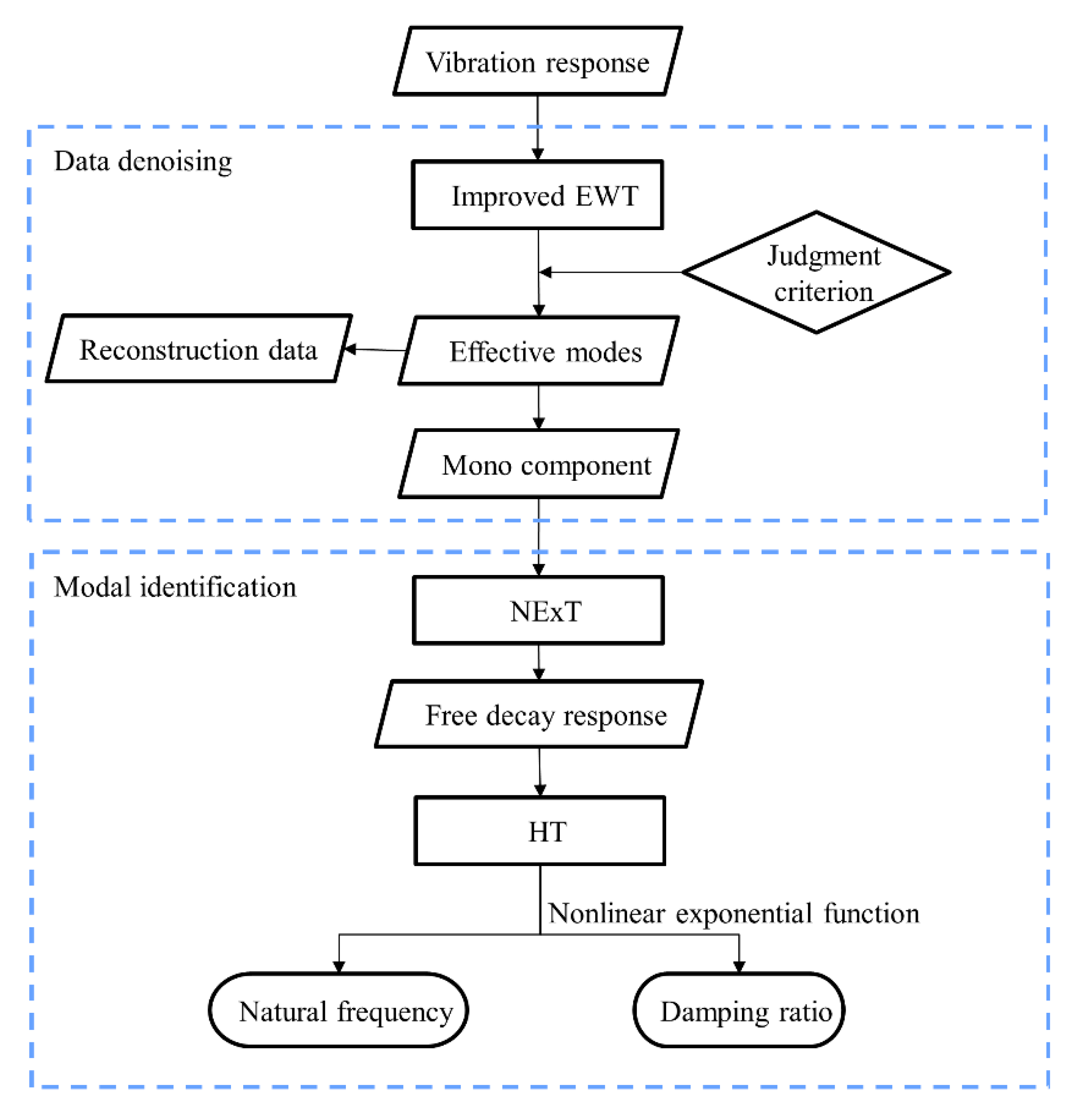
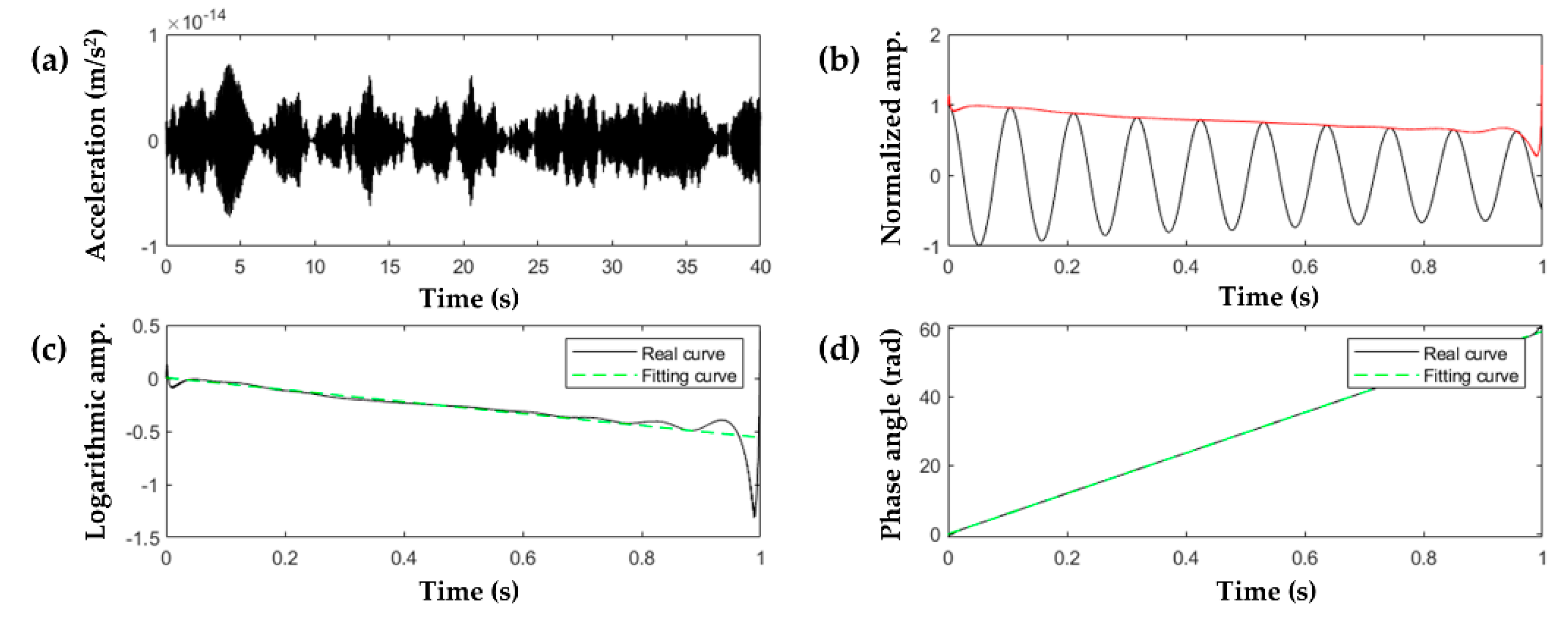
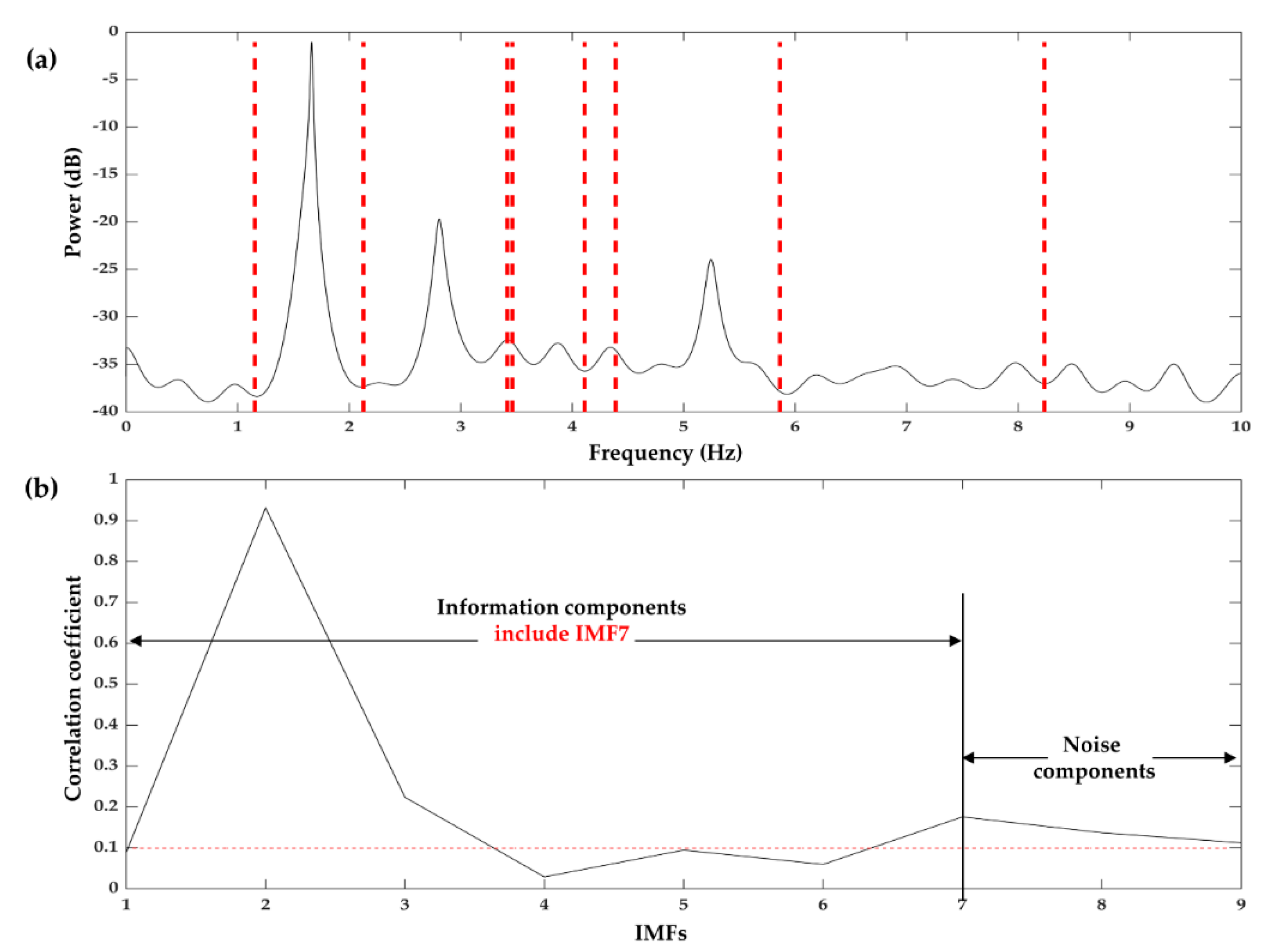
2.2. Modal Parameters Identification Based on the Improved EWT

The improved EWT method has been successfully utilized for decomposing the multi-frequency data of structure vibration into a series of mono-frequency IMFs. Therefore, the issue of modal parameters identification is transformed from multi-Degrees-of-Freedom (DOFs) system parameters identification to Single-Degree-of-Freedom (SDOF). With the individual IMF from the improved EWT method, NExT is applied to estimate the free decay response of each IMF. Once the free decay response of the mono component is estimated, HT is adopted to calculate the envelope of each free decay response to further determine the NF. Afterwards, a nonlinear exponential function is used to fit the envelope for computing the DR of each component. The modal parameters identification process based on the improved EWT is shown in Figure 3.
When the vibration responses of civil structures under environmental excitation are decomposed into various IMFs using the improved EWT, NExT [33] is used to estimate the free decay response of each individual mono component, which can be expressed by Equation (10):
u R f ( t ) = R i j k ( τ ) = E [ x i k ( t + τ ) x j k ( t ) ] ,
where, u R f ( t ) represents the free decay response of IMFR, R i j k ( τ ) denotes the correlation function, and moreover, x i k ( t ) and x j k ( t ) are the response of the measuring points i and j , respectively. The core of NExT is that the correlation function between two points of a structure is similar to the free decay response under white noise excitation. Hence, the correlation function can be used instead of the free decay response to identify the modal parameters.
Each estimated free decay response u R f ( t ) has a narrow frequency band corresponding to the extracted IMFR. The analytical signal of u R f ( t ) can be written as follows:
A R ( t ) e ξ R θ R t = u R f ( t ) + j H [ u R f ( t ) ] ,
where, A R ( t ) and θ R are the instantaneous amplitude and phase angle of the free decay response u R f ( t ) . H [ u R f ( t ) ] is the Hilbert transform of u R f ( t ) .
The traditional HT estimates the instantaneous amplitude logarithmic curve and phase curve of u R f ( t ) . Then, the NF and DR of bridge structures are obtained according to the linear least-squares fit procedure. However, the recognition accuracy of DR is difficult to guarantee since time-domain identification methods are susceptible to the interference of external noise and may produce a large deviation. Therefore, a nonlinear exponential function is applied to fit the exponentially decaying curve for calculating the DR of each IMF precisely. The nonlinear exponential model and the identification of DR can be expressed as follows:
G f i t t e d ( t ) = A R e b t ,
ξ R = b θ R ,
in which A ^ R represents the fitted amplitude of the free decay response of IMFR, and b defines the decay rate of the exponential function.

3. Numerical Studies

For the feasibility and effectiveness of the improved EWT-based method, the vibration responses of a four-storey steel frame model, and the acceleration response data of a suspension bridge are provided in this section.

3.1. Numerical Study on a 4-Storey Steel Frame Model

The Digital Environment for Enabling Data-Driven Science (NEEDS) datasets provide a 4-storey, 2 × 2 bay, 3D steel-frame structure benchmark model, as shown in Figure 4, which is used for related research on building structural health monitoring under external excitations [34]. A 12-DOFs finite element model code in MATLAB provided by Johnson et al. [35] was employed to simulate the dynamic response. Each floor was subject to environmental excitation in the form of white noise, perpendicular to the central column. The vibration data were measured by 16 accelerometers placed in the x- and y-directions on each floor. These sensors recorded the data for a duration of 20 s using a sampling rate of 1000 Hz and the damping ratio was assumed as 1% for each mode of the frame model. Moreover, 10% of the largest structural response root mean square (RMS) was added as noise. Figure 5a shows the time–history response of sensor 9 in the x-direction and the corresponding Yule–Walker power spectral density estimate is displayed in Figure 5b.
Considering that the inherent modes of the structure were mainly concentrated from 0~100 Hz, a 100 Hz lowpass filter was applied to the acceleration response for a better separation of the closely spaced modes. An auto-power spectrum, based on the Yule–Walker algorithm and the Fourier amplitude spectrum of the filtered simulation time–history response, were jointly adopted to calculate the boundaries. We fixed a prior number of segments, N = 10, and no global trend removal, as well as smoothing operations, for the improved EWT. The frequency segment results are shown in Figure 6.
As shown in Figure 6, in the range from 0~100 Hz, the Fourier spectrum is divided into 10 frequency bands. The frequency band division results obtained using the improved EWT method do not cause modal aliasing and have a good segmentation. Furthermore, IMF10 belongs to a noise component and IMF 1,5,7,8,9 are pseudo components whose correlation coefficient is less than 0.1, as displayed in Figure 7. According to the judgment criteria, these IMFs do not participate in the subsequent identification of modal parameters.
Based on the defined boundaries, the corresponding wavelet filter bank is established, and the original data is decomposed into several mono individual components through EWT. Taking IMF2 as an example (see Figure 8a), the free decay response is obtained through NExT, and then the HT is applied to determine the envelop of the free decay response (see Figure 8b). Besides, the logarithmic amplitude and phase angle representation are fitted by the least square algorithm (see Figure 8c,d). The NF and DR estimated by the HT are 9.4051 Hz and 0.92%, respectively. The DR, using the nonlinear exponential function, is 0.96%, which is closer to the theoretical value. The modal parameters information and corresponding theoretical values of the remaining meaningful IMF are shown in Table 1.
In addition, the measured frequencies of the pseudo components IMF5, 7, and 8 are 38.6387, 56.7514, and 66.6769 Hz, respectively, which are within 1% of the FEA results. This phenomenon proves that the pseudo components also contain useful information about the structure. The DRs of three sets of pseudo components are 1.17%, 2.35%, and 2.71%, respectively; the error from the theoretical value increases with the frequency. In summary, the improved EWT-based methodology can accurately identify the modal parameters of the closely spaced modes, with an NF error of less than 1% and a DR error of less than 5%. Meanwhile, the pseudo components were found to contain useful information regarding the structure. However, due to the small value of the correlation coefficient, there is a certain error between the recognized modes and the FEA values.

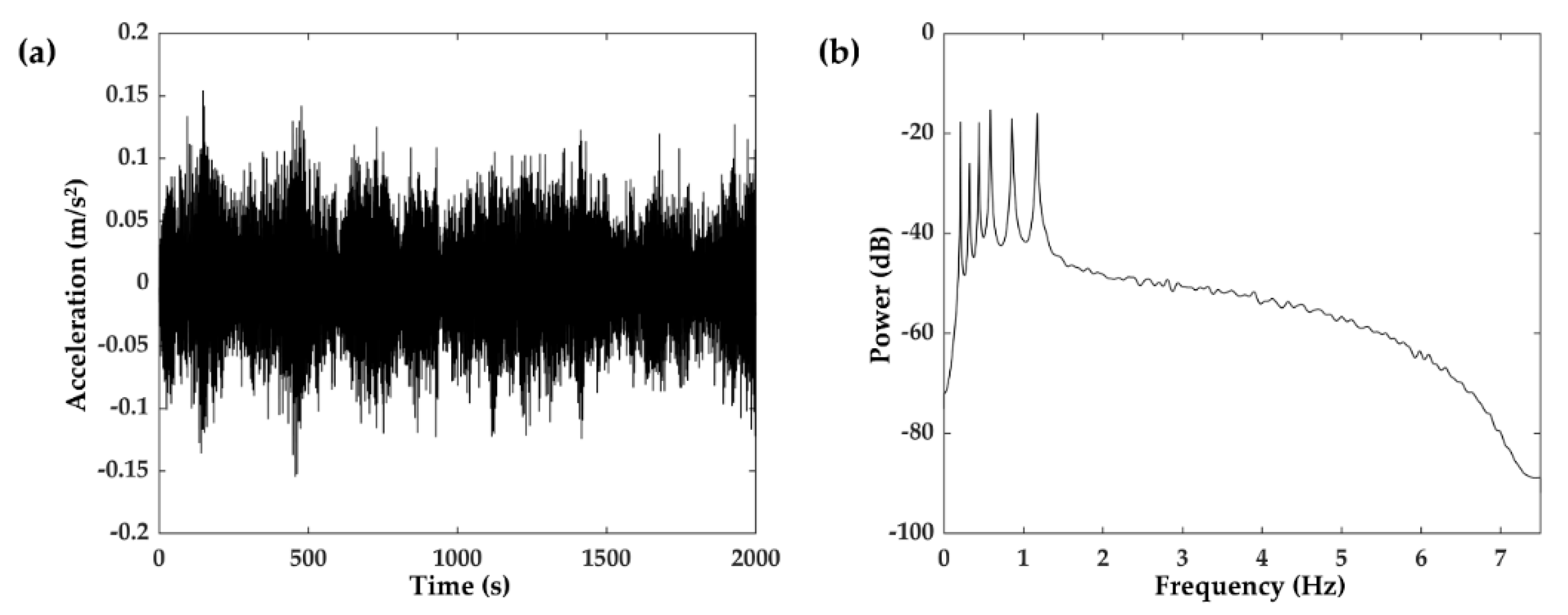
3.2. Numerical Study on Acceleration Response Data of a Suspension Bridge

Cheynet et al. [36] established a simple model of the Lysefjord suspension bridge based on the long-term monitoring data. The acceleration-response data were based on simulated displacement records which were recorded by a sampling frequency of 15 Hz for a duration of 2000 s. Figure 9 shows the time–history responses of the acceleration data and its power spectrum.
Figure 10a shows the segmentation results of the Fourier spectrum determined by the improved EWT method, and the obtained EWT component is shown in Figure 10b. According to the effective component judgment criteria, the reconstructed components IMF 2~7 are effective components. Using the improved EWT-based procedure, the modal parameters of the Lysefjord suspension bridge are identified. For a comparison with the results of the proposed method, the target values of corresponding modal parameters are also provided in Table 2.
It is noted that the first five modal parameters identified by the proposed method are essentially consistent with the target values. The NF identification error is less than 0.1%, and the highest error of DR does not exceed 8%. However, with the increasing frequency, the NF error of mono individual components is increased to 2%, and the DR error of high-order modes exceeds 10%. This may be related to the interference of high-frequency noise.

4. Field Experiments

4.1. Engineering Background

In this section, the proposed method is used to process the forced vibration data of the Wilford footbridge, which is a self-anchored suspension bridge with double main cable located in Nottingham, UK. The main span length of this bridge is 69 m, and the width is 3.7 m. In order to monitor the vibration responses of this bridge structure, the main instrumentation employed in the experiments included three sets of GS10 GNSS receivers with a sampling rate of 20 Hz, a Kistler 8392A2 tri-axial accelerometer with a sampling rate of 100 Hz, a precise time–data logger, a signal splitter, a Leica AR10 antenna (used on the monitoring site) and a Leica AT504 choke-ring antenna (used at the reference station). Five monitoring experiments, which mainly recorded the dynamic responses of the structure under the synchronous jumping excitation of the experimenters, were carried out on this suspension bridge. For more details about this field of experiments, refer to Yu et al. [37,38]. In the field experiments, the instruments placement is shown in Figure 11.
The kinematic solution methods of the GNSS data adopted three data-processing modes (real-time kinematic, network real-time kinematic, and post-processing kinematic). The real-time kinematic (RTK) mode received correction differences sent by an independent reference station (3# receiver) set up at the riverside near the bridge, about 60 m away. Whereas the network RTK (NRTK) used the correction differences from the Smart NET CORS system in United Kingdom. Both kinematic solution methods transmitted the corrections at the updating rate of 1 Hz. The monitoring site was located on the downstream side of the mid-span of the bridge. The receivers, 1# and 2#, were connected to the Leica AR10 antenna through a signal splitter, which enabled the receivers to synchronously acquire GNSS data (SRTK, SNRTK). The accelerometer was kept coaxial with the GNSS antenna and the center of the base through a cage monitoring device, by rotating the upper and lower plate, where one axis of the accelerometer was parallel to the longitudinal axis of the bridge. The forced vibrations were excited by three experimenters with a total weight of 180 kg jumping synchronously for 10 s every 3 min at the mid-span of the bridge. During the field experiments, the GNSS receivers received only GPS satellite signals with an elevation cutoff angle of 15 degrees. Using the above sensors, three groups of monitoring data were collected simultaneously (SRTK, SNRTK, SACC). To verify the proposed method, the GNSS and accelerometer (ACC) data covering approximately 12 min were selected. Taking the z-direction as an example, Figure 12 shows the time–history of the data observed by GNSS for a total of 14,400 epochs, and the accelerometer data.

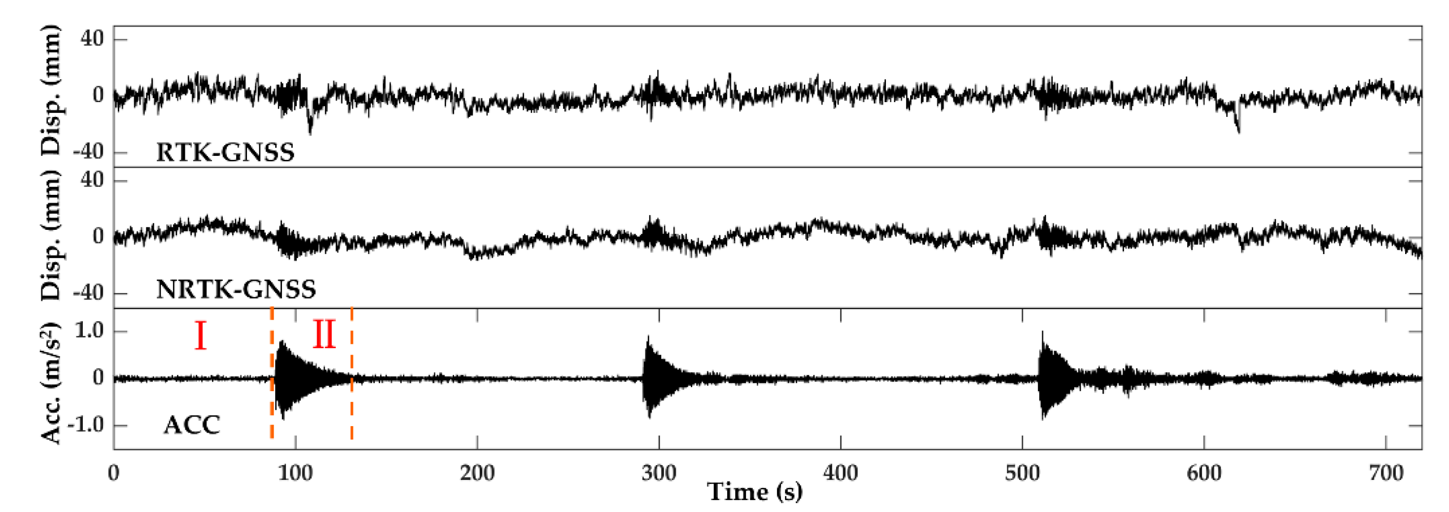
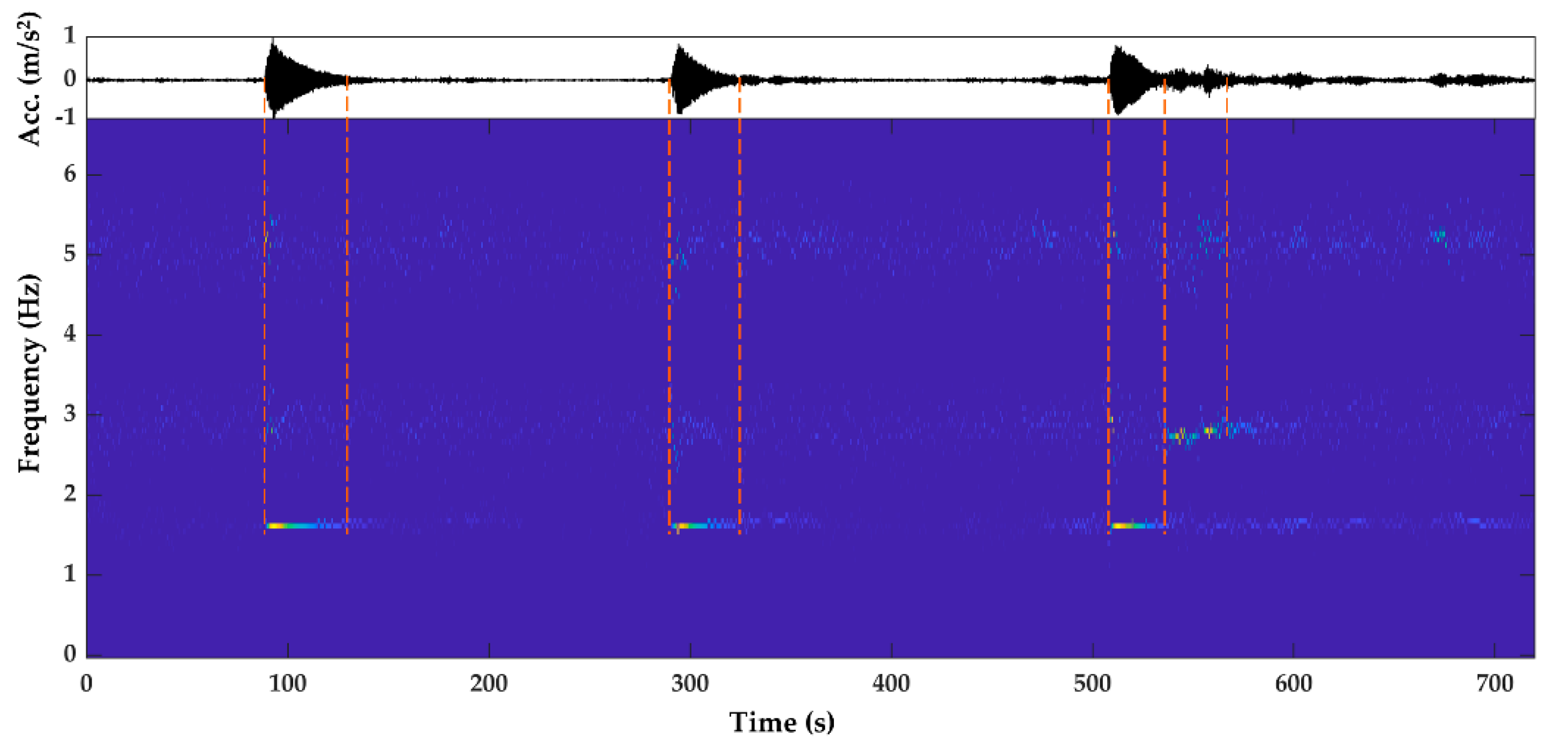
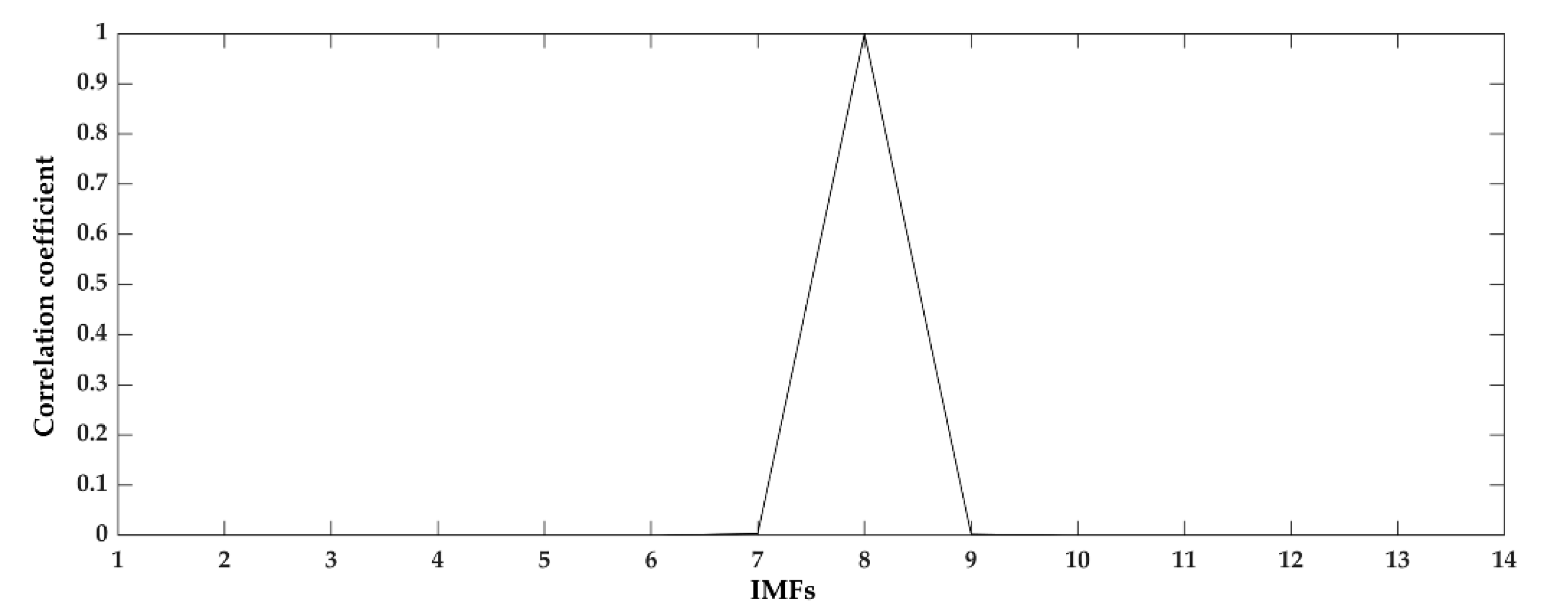
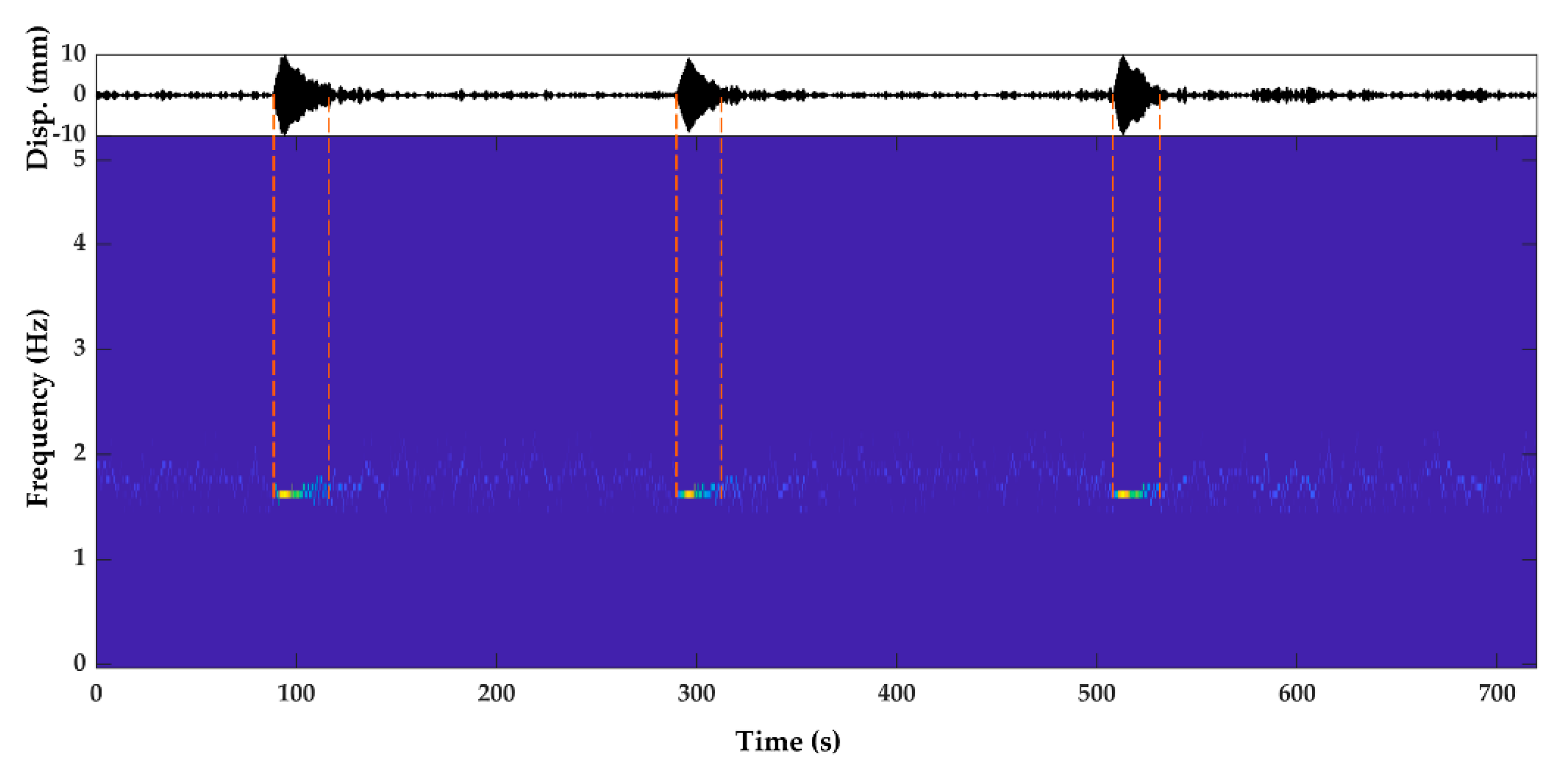
4.2. Data Processing and Analysis

As shown in Figure 12, the actual vibration responses from the ACC data SACC of the bridge are divided into two parts. Part one is the random vibration caused by environmental excitation, and part two is the forced vibration under synchronous jumping excitation of three experimenters weighing 180 kg. In the first step, according to the improved algorithm, the meaningful dynamic displacement and various modal parameters are extracted from the ACC data.
Figure 13a,b shows the power-spectrum frequency-band division results and correlation coefficient distribution diagram of the accelerometer. Three obvious peaks can be observed in the power spectrum and its corresponding frequencies, at 1.662, 2.798, and 5.243 Hz. Furthermore, IMF8, 9 belongs to noise components and IMF 1, 4~6 are pseudo components whose correlation coefficient is less than 0.1, as displayed in Figure 13b. According to the judgment criteria, the remaining IMF 2, 3, and 7 are the effective modes. Furthermore, the modal parameters of these effective modes are identified using the improved EWT-based method, shown as Table 3. The error between the identified modal frequencies and the peak values extracted from the power spectral density is within 2%, which is relatively consistent. The time–frequency (TF) representation of meaningful components of SACC is displayed in Figure 14. The structural vibration effect caused by the jumping excitation on the time–history response is consistent with the time–frequency response of IMF2, indicating that the modal parameters of this component are related to the jumping excitation. The brightness for the instantaneous frequency lines of IMF3 at 540~570 s is very high, which is consistent with the fluctuation of the time–history curve, confirming that modal parameters of this component are related to environmental excitation.
NRTK obtains high-quality continuous observation data and establishes an accurate differential calculation model through the establishment of the continuous operation reference station (CORS) network system. It realizes the real-time dynamic high-precision relative positioning of the rover station, and its positioning accuracy can achieve the accuracy of the traditional RTK short baseline [1]. However, the time–history of RTK data appears to be an abnormal displacement [38]. In order to accurately extract the NF and DR of the bridge, the NRTK-GNSS monitoring data are analyzed.
Due to the influence of long-period displacement and various noise, the structural vibration characteristics monitored by GNSS are cloaked by noise. As shown in Figure 12, the waveforms of the GNSS data and the accelerometer data are clearly different. The dynamic displacement component obtained by the improved EWT has little correlation with the original data. However, the low-frequency component of the data (long period displacement, multipath error, etc.) shows a good correlation with the original data. Hence, the modal parameters identification could be successfully addressed to the GNSS data only after removing the low-frequency components of long-period displacement and multipath error. Meng et al. [39] measured the fundamental frequency of the Wilford bridge as 1.733 Hz from the response measurements of decayed free vibration in 2003. After the restoration of this bridge, Yu et al. [38] re-identified the vibration mode of the bridge and found that the fundamental frequency was 1.690 Hz. Based on the experimental results of the above scholars, the minimum modal frequency of the Wilford bridge should be about 1.700 Hz. Considering the influence of GNSS low-frequency noise, the low-frequency components whose boundaries are less than 1.700 Hz need to be removed when the mono individual mode is defined as using the improved EWT method, and the effective IMFs are detected by the proposed criteria. The spectrum segmentation and correlation coefficient diagrams of NRTK-GNSS are shown in Figure 15. Based on the judgment criteria, IMF1, 2, 3, 6, and 8 are effective components before reconstruction. After removing the frequency band of less than 1.700 Hz, only IMF8 remains the effective component, and the correlation coefficients of other components with the reconstructed data tend to be 0, as presented in Figure 16. Subsequently, the NF and DR of IMF8, identified using the improved EWT-based method, are 1.6707 Hz and 0.84%, respectively. The error of the fundamental frequency and damping ratio between NRTK-GNSS and the accelerometer’s result is 0.02% and 2.38%, separately. Moreover, the difference between NRTK-GNSS and Meng et al. [39] is less than 5%, which satisfies the limitation. Figure 17 shows the TF representation of the effective components of NRTK-GNSS. The vibration displacement generated by the jumping excitation is consistent with the brightness duration of the instantaneous frequency line, as well as the time–frequency diagram of the ACC data.
Figure 18 shows the NRTK-GNSS dynamic displacement derived by the improved EWT-based method and the acceleration dynamic displacement obtained by double integration in the frequency domain. It is noted that the waveforms of the two groups of displacement curves after noise reduction are similar. In order to evaluate the noise reduction effect, the NRTK-GNSS data are used as noise data; meanwhile, the dynamic displacement derived from the accelerometer is used as ideal data. The EMD algorithm and WT algorithm are compared with the proposed method, and the evaluation indicators throw light on the noise reduction effect of different methods, namely, signal-to-noise ratio (SNR), root mean square error (RMSE) and the correlation coefficient (R). Table 4 enlists the statistical results for the above methods. It reveals that the R, RMSE and SNR of the proposed method are superior to the other two methods, which confirm that the proposed method could effectively remove multipath error, random noise and maintain the meaningful data.
The maximum vibration displacement is an important index to evaluate the safety performance of bridge structure. The maximum dynamic displacements of the NRTK, RTK data, extracted using the improved EWT method, are 10.10 mm and 10.40 mm, respectively. Besides, as the verification group, the maximum dynamic displacement calculated by the accelerometer is 9.42 mm. The monitoring difference between two sensors is lower than 1.0 mm after data processing. As shown in Figure 18, there are three obvious peak ranges in the displacement curve. Figure 19 shows that the dynamic displacement of NRTK-GNSS and the accelerometer in the E2 interval (288~300 s). In this range, the correlation coefficient of the bridge’s dynamic displacement, derived from the GNSS and ACC data, is 0.9343, which indicates that these two coordinate time series are very similar. The standard deviation of displacement between NRTK and the accelerometer is less than 2.0 mm. The accuracy is sufficient enough for structural health monitoring.

5. Conclusions

In order to effectively reduce the noise of bridge GNSS monitoring data and identify the structural modal parameters, this paper proposed an improved EWT-based method. The vibration responses of a four-storey steel frame model, acceleration response data of the Lysefjord bridge, and a Wilford bridge experimental study were employed to illustrate the efficiency of the proposed method. Moreover, the denoising ability of the proposed method was evaluated in comparison with the EMD and WT algorithm. In the numerical examples, the improved EWT, building boundaries using the Yule–Walker algorithm-based auto-power spectrum, combined with the Fourier spectrum, could identify the structural low-order, closely spaced modes. The modal parameters error of NF and DR was less than 2% and 10%, respectively. However, the DR of high-order components could not be measured accurately because of the existence of high-frequency noise. In the field experiments, the first three modal parameters of the Wilford bridge were extracted from the accelerometer data using the improved EWT-based procedure. Due to the low sampling frequency of the GNSS receiver, only a group of the modal parameters of 1.6707 Hz and 0.84% were identified from the NRTK-GNSS monitoring data, which was less than 5% in the fundamental frequency error compared with the error detected by Meng et al. [39]. Moreover, the DR error between the NRTK-GNSS and the accelerometer result was 2.38%. The maximum dynamic displacements (10.10 mm) of the Wilford bridge were successfully derived from the NRTK-GNSS.
The first contribution of this study was that the feasibility of using the improved EWT-based method for data denoising was validated. The power spectrum calculated by the Yule–Walker algorithm combined with the Fourier spectrum could divide the frequency band properly. The proposed judgment criteria could separate effective modes from a series of components. Moreover, the effect of data denoising and dynamic displacements reconstruction was superior to the EMD and WT method.
In addition, the feasibility of using the improved EWT-based procedure for the identification of modal parameters was proven in the experiment presented herein. The low-order NFs and DRs of a four-storey steel-frame model and the Lysefjord bridge model were identified accurately. Moreover, its DR identification results were better than the estimation of Zhou et al. [7] in the first four modes of the Lysefjord bridge. However, the DR of high-frequency components was an uncertain parameter. According to this method, the fundamental frequency and first-order damping ratio of the Wilford footbridge were effectively identified from NRTK-GNSS monitoring data, which were verified by accelerometer identification results.
The improved empirical wavelet transform would therefore be a promising tool of denoising GNSS data, as well as identifying structural modal parameters. In this study, the proposed method is capable of accurately identifying the low-order, closely spaced modal parameters of bridge structures. However, the DR error of high-order modes is large since the effective components extracted by improved EWT still contained noise. Further research needs to be conducted on the combination of EWT with other algorithms to denoise data further.

Author Contributions

Conceptualization, J.Y. and X.M.; methodology, J.Y. and Z.F.; formal analysis, Z.F.; data curation, J.Y.; writing—original draft preparation, Z.F.; writing—review and editing, J.Y. and X.M.; supervision, X.M.; project administration, J.Y. and X.M.; funding acquisition, J.Y. All authors have read and agreed to the published version of the manuscript.

Funding

This research was funded by Changsha science and technology project (No. kq1907110), Hunan Water Resources Science and Technology project (No. XSKJ2021000-46), Hunan Provincial Natural Science Foundation of China (No. 2021JJ30102) and Hunan commercialization of research findings and industrialization plan (No. 2020GK2026).

Data Availability Statement

The four-storey steel frame model and corresponding MATLAB codes are available on the web site at https://datacenterhub.org/resources/257 (accessed on 12 May 2021).

Acknowledgments

The University of Nottingham is thanked for supplying instruments in field experiments.

Conflicts of Interest

The authors declare no conflict of interest.

Abbreviations

AbbreviationThe Full Name
GNSSGlobal Navigation Satellite System
EWTEmpirical Wavelet Transform
NExTNatural Excitation Technique
HTHilbert Transform
WTWavelet Transform
CWTContinuous Wavelet Transform
LSWALeast-Squares Wavelet Analysis
WWAWeighted Wavelet Analysis
EMDEmpirical Mode Decomposition
EEMDEnsemble Empirical Mode Decomposition
MEMDMultivariate Empirical Mode Decomposition
IMFIntrinsic Mode Function
MUSICMultiple Signal Classification
NFNatural Frequency
DRDamping Ratio
SETSynchro-Extracting Transform
LWMLocal Window Maxima
AM-FMAmplitude Modulation-Frequency Modulation
DOFDegrees-of-Freedom
FEAFinite Element Analysis
RTKReal-Time Kinematic
NRTKNetwork Real-Time Kinematic
PPKPost-Processing Kinematic
CORSContinuous Operation Reference Station
ACCAccelerometer
TFTime–frequency
SNRSignal-to-Noise Ratio
RMSERoot Mean Square Error
RCorrelation Coefficient

References

  1. Shen, N.; Chen, L.; Liu, J.B.; Wang, L.; Tao, T.Y.; Wu, D.W.; Chen, R.Z. A review of Global Navigation Satellite System (GNSS)-based dynamic monitoring technologies for structural health monitoring. Remote Sens. 2019, 11, 1001. [Google Scholar] [CrossRef] [Green Version]
  2. Moschas, F.; Stiros, S. Dynamic deflections of a stiff footbridge using 100-Hz GNSS and accelerometer data. J. Surv. Eng. 2015, 141, 04015003. [Google Scholar] [CrossRef]
  3. Yu, J.Y.; Meng, X.L.; Yan, B.F.; Xu, B.; Fan, Q.; Xie, Y.L. Global Navigation Satellite System-based positioning technology for structural health monitoring: A review. Struct. Control Health Monit. 2020, 27, e2467. [Google Scholar] [CrossRef] [Green Version]
  4. Gaxiola-Camacho, J.R.; Bennett, R.; Guzman-Acevedo, G.M.; Gaxiola-Camacho, I.E. Structural evaluation of dynamic and semi-static displacements of the Juarez Bridge using GPS technology. Measurement 2017, 110, 146–153. [Google Scholar] [CrossRef]
  5. Xi, R.J.; Chen, H.; Meng, X.L.; Jiang, W.P.; Chen, Q.S. Reliable dynamic monitoring of bridges with integrated GPS and BeiDou. J. Surv. Eng. 2018, 144, 04018008. [Google Scholar] [CrossRef]
  6. Yu, L.N.; Xiong, C.B.; Gao, Y.; Zhu, J.S. Combining GNSS and accelerometer measurements for evaluation of dynamic and semi-static characteristics of bridge structures. Meas. Sci. Technol. 2020, 31, 125102. [Google Scholar] [CrossRef]
  7. Zhou, W.; Feng, Z.R.; Liu, D.S.; Wang, X.J.; Chen, B.B. Modal parameter identification of structures based on short-time narrow-banded mode decomposition. Adv. Struct. Eng. 2020, 23, 3062–3074. [Google Scholar] [CrossRef]
  8. Fan, Q.; Meng, X.L.; Nguyen, D.T.; Xie, Y.L.; Yu, J.Y. Predicting displacement of bridge based on CEEMDAN-KELM model using GNSS monitoring data. J. Appl. Geod. 2020, 14, 253–261. [Google Scholar] [CrossRef]
  9. Kaloop, M.R.; Hussan, M.; Kim, D. Time-series analysis of GPS measurements for long-span bridge movements using wavelet and model prediction techniques. Adv. Space Res. 2019, 63, 3505–3521. [Google Scholar] [CrossRef]
  10. Kaczmarek, A.; Kontny, B. Identification of the noise model in the time series of GNSS stations coordinates using wavelet analysis. Remote Sens. 2018, 10, 1611. [Google Scholar] [CrossRef] [Green Version]
  11. Ji, K.; Shen, Y.; Wang, F. Signal extraction from GNSS position time series using weighted wavelet analysis. Remote Sens. 2020, 12, 992. [Google Scholar] [CrossRef] [Green Version]
  12. Ghaderpour, E.; Ghaderpour, S. Least-squares spectral and wavelet analyses of V455 Andromedae time series: The life after the super-outburst. Publ. Astron. Soc. Pac. 2020, 132, 114504. [Google Scholar] [CrossRef]
  13. Barbosh, M.; Singh, P.; Sadhu, A. Empirical mode decomposition and its variants: A review with applications in structural health monitoring. Smart Mater. Struct. 2020, 29, 093001. [Google Scholar] [CrossRef]
  14. Civera, M.; Surace, C. A comparative analysis of signal decomposition techniques for structural health monitoring on an experimental benchmark. Sensors 2021, 21, 1825. [Google Scholar] [CrossRef] [PubMed]
  15. Huang, N.E.; Shen, Z.; Long, S.R.; Wu, M.C.; Shih, H.H.; Zheng, Q.; Yen, N.-C.; Tung, C.C.; Liu, H.H. The empirical mode decomposition and the Hilbert spectrum for nonlinear and non-stationary time series analysis. Proc. R. Soc. Lond. Ser. A Math. Phys. Eng. Sci. 1998, 454, 903–995. [Google Scholar] [CrossRef]
  16. Hu, Y.; Li, F.; Li, H.; Liu, C. An enhanced empirical wavelet transform for noisy and non-stationary signal processing. Digit. Signal Process. 2017, 60, 220–229. [Google Scholar] [CrossRef]
  17. Gilles, J. Empirical wavelet transform. IEEE Trans. Signal Process. 2013, 61, 3999–4010. [Google Scholar] [CrossRef]
  18. Gilles, J.; Heal, K. A parameterless scale-space approach to find meaningful modes in histograms—Application to image and spectrum segmentation. Int. J. Wavelets Multiresolut. Inf. Process. 2014, 12, 1450044. [Google Scholar] [CrossRef]
  19. Akbari, H.; Sadiq, M.T.; Rehman, A.U. Classification of normal and depressed EEG signals based on centered correntropy of rhythms in empirical wavelet transform domain. Health Inf. Sci. Syst. 2021, 9, 1–15. [Google Scholar] [CrossRef]
  20. Liao, Z.R.; Zhang, Y.F.; Li, Z.Y.; He, B.B.; Lang, X.; Liang, H.; Chen, J.H. Classification of red blood cell aggregation using empirical wavelet transform analysis of ultrasonic radiofrequency echo signals. Ultrasonics 2021, 114, 106419. [Google Scholar] [CrossRef]
  21. Liu, H.; Yu, C.Q.; Wu, H.P.; Duan, Z.; Yan, G.X. A new hybrid ensemble deep reinforcement learning model for wind speed short term forecasting. Energy 2020, 202, 117794. [Google Scholar] [CrossRef]
  22. Kalra, M.; Kumar, S.; Das, B. Seismic signal analysis using Empirical Wavelet Transform for moving ground target detection and classification. IEEE Sens. J. 2020, 20, 7886–7895. [Google Scholar] [CrossRef]
  23. Yu, H.; Li, H.R.; Li, Y.L. Vibration signal fusion using improved empirical wavelet transform and variance contribution rate for weak fault detection of hydraulic pumps. ISA Trans. 2020, 107, 385–401. [Google Scholar] [CrossRef]
  24. Amezquita-Sanchez, J.P.; Park, H.S.; Adeli, H. A novel methodology for modal parameters identification of large smart structures using MUSIC, empirical wavelet transform, and Hilbert transform. Eng. Struct. 2017, 147, 148–159. [Google Scholar] [CrossRef]
  25. Amezquita-Sanchez, J.P.; Adeli, H. A new music-empirical wavelet transform methodology for time-frequency analysis of noisy nonlinear and non-stationary signals. Digit. Signal Process. 2015, 45, 55–68. [Google Scholar] [CrossRef]
  26. Xin, Y.; Hao, H.; Li, J. Operational modal identification of structures based on improved empirical wavelet transform. Struct. Control Health Monit. 2019, 26, e2323. [Google Scholar] [CrossRef]
  27. Xia, Y.X.; Zhou, Y.L. Mono-component feature extraction for condition assessment in civil structures using empirical wavelet transform. Sensors 2019, 19, 4280. [Google Scholar] [CrossRef] [Green Version]
  28. Xin, Y.; Hao, H.; Li, J. Time-varying system identification by enhanced empirical wavelet transform based on synchroextracting transform. Eng. Struct. 2019, 196, 109313. [Google Scholar] [CrossRef]
  29. Dong, S.; Yuan, M.; Wang, Q.; Liang, Z. A modified empirical wavelet transform for acoustic emission signal decomposition in structural health monitoring. Sensors 2018, 18, 1645. [Google Scholar] [CrossRef] [PubMed] [Green Version]
  30. Zhao, L.; He, Y. The power spectrum estimation of the AR model based on motor imagery EEG. In Mechatronics and Intelligent Materials Iii, Pts 1-3; Chen, R., Sung, W.P., Kao, J.C.M., Eds.; Advanced Materials Research; Trans Tech Publications Ltd.: Stafa-Zurich, Switzerland, 2013; Volumes 706–708, pp. 1923–1927. [Google Scholar]
  31. Xue, B.; Hong, H.; Zhou, S.; Chen, G.; Li, Y.; Wang, Z.; Zhu, X. Morphological filtering enhanced empirical wavelet transform for mode decomposition. IEEE Access 2019, 7, 14283–14293. [Google Scholar] [CrossRef]
  32. Liu, X.L.; Jiang, M.Z.; Liu, Z.Q.; Wang, H. A morphology filter-assisted extreme-point symmetric mode decomposition (MF-ESMD) denoising method for bridge dynamic deflection based on ground-based microwave interferometry. Shock Vib. 2020, 2020, 8430986. [Google Scholar] [CrossRef]
  33. Pei, Q.; Li, L. Structural modal parameter identification based on natural excitation technique. In Advanced Research on Civil Engineering, Materials Engineering and Applied Technology; Zhang, H., Jin, D., Zhao, X.J., Eds.; Advanced Materials Research; Trans Tech Publications Ltd.: Stafa-Zurich, Switzerland, 2014; Volume 859, pp. 167–170. [Google Scholar]
  34. Dyke, S.; Agrawal, A.K.; Caicedo, J.M.; Christenson, R.; Gavin, H.; Johnson, E.; Nagarajaiah, S.; Narasimhan, S.; Spencer, B. NEES: Database for Structural Control and Monitoring Benchmark Problems. 2015. Available online: https://datacenterhub.org/resources/257 (accessed on 12 May 2021).
  35. Johnson, E.A.; Lam, H.F.; Katafygiotis, L.S.; Beck, J.L. Phase I IASC-ASCE structural health monitoring benchmark problem using simulated data. J. Eng. Mech. 2004, 130, 3–15. [Google Scholar] [CrossRef]
  36. Cheynet, E.; Daniotti, N.; Jakobsen, J.B.; Snæbjörnsson, J. Improved long-span bridge modeling using data-driven identification of vehicle-induced vibrations. Struct. Control Health Monit. 2020, 27, e2574. [Google Scholar] [CrossRef]
  37. Yu, J.Y.; Meng, X.L.; Shao, X.D.; Yan, B.F.; Yang, L. Identification of dynamic displacements and modal frequencies of a medium-span suspension bridge using multimode GNSS processing. Eng. Struct. 2014, 81, 432–443. [Google Scholar] [CrossRef]
  38. Yu, J.Y.; Yan, B.F.; Meng, X.L.; Shao, X.D.; Ye, H. Measurement of bridge dynamic responses using network-based real-time kinematic GNSS technique. J. Surv. Eng. 2016, 142, 04015013. [Google Scholar] [CrossRef]
  39. Meng, X.L.; Dodson, A.H.; Roberts, G.W. Detecting bridge dynamics with GPS and triaxial accelerometers. Eng. Struct. 2007, 29, 3178–3184. [Google Scholar] [CrossRef]
Figure 1. Flowchart of data denoising and modal parameters identification.
Remotesensing 13 03375 g001
Figure 2. Flowchart of the improved EWT.
Remotesensing 13 03375 g002
Figure 3. Flowchart of modal parameters identification based on the improved EWT.
Remotesensing 13 03375 g003
Figure 4. Scale model structure of steel frame.
Remotesensing 13 03375 g004
Figure 5. Time–history response of sensor 9 in the x-direction and its power spectrum: (a) time–history response and (b) Yule–Walker power spectral density estimate.
Remotesensing 13 03375 g005
Figure 6. Segmentation of the Fourier spectrum.
Remotesensing 13 03375 g006
Figure 7. Correlation coefficient distribution diagram.
Remotesensing 13 03375 g007
Figure 8. Modal parameters identification of IMF2: (a) time–history response of IMF2; (b) free vibration response and envelop; (c) logarithmic amplitude curve and (d) phase angle curve.
Remotesensing 13 03375 g008
Figure 9. Time–history response and power spectrum of Lysefjord suspension bridge: (a) time–history response and (b) Yule–Walker power spectral estimate.
Remotesensing 13 03375 g009
Figure 10. Segmentation of the Fourier spectrum and the decomposed EWT components: (a) segmentation of Fourier spectrum and (b) decomposed EWT components.
Remotesensing 13 03375 g010aRemotesensing 13 03375 g010b
Figure 11. The Wilford suspension bridge and the instrumentation layout.
Remotesensing 13 03375 g011
Figure 12. Time–history of GNSS and the accelerometer in the z-direction.
Remotesensing 13 03375 g012
Figure 13. Spectrum segmentation and correlation coefficient distribution diagram of ACC data: (a) segmentation of power spectrum and (b) correlation coefficient distribution map.
Remotesensing 13 03375 g013
Figure 14. TF plane of the effective modes of ACC data.
Remotesensing 13 03375 g014
Figure 15. Spectrum segmentation and correlation coefficient diagram of NRTK-GNSS: (a) segmentation of power spectrum and (b) correlation coefficient distribution map.
Remotesensing 13 03375 g015
Figure 16. Correlation coefficient distribution diagram after reconstruction.
Remotesensing 13 03375 g016
Figure 17. TF plane of the effective modes of NRTK-GNSS.
Remotesensing 13 03375 g017
Figure 18. Dynamic displacements derived from the GNSS and ACC data.
Remotesensing 13 03375 g018
Figure 19. Comparison of the dynamic displacement in E2 interval: (a) dynamic displacement of NRTK-GNSS and ACC and (b) the displacement difference between NRTK-GNSS and ACC.
Remotesensing 13 03375 g019
Table 1. Modal parameters identification results of the frame model.
IMFFEAProposed MethodDifference
NF (Hz)DR (%)NF (Hz)DR (%)NF (%)DR (%)
29.411.09.40510.960.054
316.381.016.35401.00.160
425.541.025.45291.020.342
648.011.047.98890.960.044
Table 2. The modal parameters identification of Lysefjord bridge.
IMFTarget ValueProposed MethodDifference
NF (Hz)DR (%)NF (Hz)DR (%)NF (%)DR (%)
20.20460.500.20460.5306
30.31890.500.31920.520.094
40.43910.500.43810.540.238
50.58520.500.58520.5408
60.86430.500.85740.670.8034
71.19440.501.17180.391.8922
Table 3. Modal parameters identification from ACC data of Wilford bridge.
ModeNF (Hz)DR (%)
11.67100.82
22.84340.48
35.20590.50
Table 4. The denoising effect of different methods.
MethodSNR (dB)RMSE (mm)R
EMD2.04241.70.6145
WT2.48351.50.6628
Proposed method8.77730.520.9343
Publisher’s Note: MDPI stays neutral with regard to jurisdictional claims in published maps and institutional affiliations.

