Feature Selection and Mislabeled Waveform Correction for Water–Land Discrimination Using Airborne Infrared Laser

Abstract

The discrimination of water–land waveforms is a critical step in the processing of airborne topobathy LiDAR data. Waveform features, such as the amplitudes of the infrared (IR) laser waveforms of airborne LiDAR, have been used in identifying water–land interfaces in coastal waters through waveform clustering. However, water–land discrimination using other IR waveform features, such as full width at half maximum, area, width, and combinations of different features, has not been evaluated and compared with other methods. Furthermore, false alarms often occur when water–land discrimination in coastal areas is conducted using IR laser waveforms because of environmental factors. This study provides an optimal feature for water–land discrimination using an IR laser by comparing the performance of different waveform features and proposes a dual-clustering method integrating K-means and density-based spatial clustering applications with noise algorithms to improve the accuracy of water–land discrimination through the clustering of waveform features and positions of IR laser spot centers. The proposed method is used for practical measurement with Optech Coastal Zone Mapping and Imaging LiDAR. Results show that waveform amplitude is the optimal feature for water–land discrimination using IR laser waveforms among the researched features. The proposed dual-clustering method can correct mislabeled water or land waveforms and reduce the number of mislabeled waveforms by 48% with respect to the number obtained through traditional K-means clustering. Water–land discrimination using IR waveform amplitude and the proposed dual-clustering method can reach an overall accuracy of 99.730%. The amplitudes of IR laser waveform and the proposed dual-clustering method are recommended for water–land discrimination in coastal and inland waters because of the high accuracy, resolution, and automation of the methods.

1. Introduction

Airborne LiDAR bathymetry (ALB) uses scanning and pulsed laser beams from air to detect shallow waters, showing high efficiency, accuracy, and resolution and economy, safety, and flexibility [1,2]. Apart from water depth measurement [3,4,5,6,7,8], ALB has been applied to water–land discrimination [9,10,11,12], suspended sediment concentration monitoring [13,14], ocean wave pattern analysis [15,16,17,18], and seabed classification [19,20,21]. Integrated infrared (IR) and green ALB systems use green laser with a wavelength of 532 nm to detect water bottom and IR laser with a wavelength of 1064 nm to detect water surface. Green-only ALB systems use green laser to detect water surface and bottom [8]. ALB systems can integrate water and land measurements and receive laser pulse returns reflected from water and land [11]. The entire sequence of the interactions of the laser pulse with water or land is recorded at the receiver as a full waveform [9]. The discrimination of water–land waveforms is a critical step in ALB laser waveform processing and can be performed for the determination of water–land interfaces [9,12], which play an important role in the management and scientific research of water and land resources in estuaries and coastal zones.

Waveform saturation judgement [1,10], red waveform analysis [22,23], waveform classification [24,25,26], and point cloud threshold or clustering [11,12] methods are primarily used in water–land discrimination. Guenther [1] proposed the waveform saturation judgement method for Optech SHOALS series to identify an IR laser waveform as land if the amplitude of the waveform is in saturation for more than 5 ns or as water if otherwise. Collin et al. [10] distinguished land waveforms from water waveforms with Guenther’s waveform saturation judgement method. The development of ALB devices has enabled analog-to-digital converters in ALB systems to record full laser waveforms [27]. Thus, the amplitudes of land signals may be unsaturated. Another problem with waveform saturation is that the IR laser waveform can also be saturated due to scattering from bubbles that occur in rolling surfs and whitecaps [9,28].

A wavelength is generated by the Raman scattering of the green pulse generated by water and produces a detectable signal in the red at 645 nm [22]. Based on this phenomenon, some ALB systems, such as the Optech SHOALS series, identify water and land by adding red channels to collect red laser pulses. Pe’eri and Philpot [23] summarized water–land discrimination methods using ALB waveforms, including IR waveform saturation, green–red–IR ratio (Cornell algorithm), red-IR peak ratio, and red standard deviation algorithms. However, red channels are not adopted in modern mainstream ALB systems, such as Optech Coastal Zone Mapping and Imaging LiDAR (CZMIL), AHAB Hawkeye III, RIEGL VQ-880-G, and Fugro LADS-MK3 [11].

The amplitude of an IR laser land waveform is much larger than that of a water waveform. Accordingly, the amplitude of an IR waveform can be used as a feature for distinguishing water from land. Supervised classification models, such as support vector machines (SVMs) [24,25,26], and unsupervised classification models, such as K-means and Fuzzy C-means clustering [12], that are based on the amplitude of IR waveforms are used in discriminating water and land waveforms. Unsupervised classification does not need sample data and is more applicable for water–land discrimination compared with supervised classification. An IR laser has a strong reflection because bubble-entrained water enables special IR laser waveforms to achieve amplitudes close to those of the typical IR laser waveforms of land [9]. These special IR laser waveforms of bubble-entrained water are incorrectly labeled as land when the amplitude of an IR waveform is applied. Furthermore, land topography causes the amplitudes of some IR/green laser waveforms of land to be similar to those of water [12]. These special IR/green laser waveforms of land are incorrectly labeled as water when the amplitude of an IR waveform is applied. The shape of the green laser waveform of water is different from that of land. The amplitudes of green laser waveforms can be used in discriminating water and land [11]. However, green laser waveforms are significantly influenced by the merge effect in very shallow waters [23], and the accuracy of water–land discrimination using green laser waveforms is low [12].

An elevation threshold method using 3D point clouds obtained with IR laser is proposed to realize rapid water–land identification [11]. This method can distinguish ocean from land but cannot effectively identify inland waters. Zhao et al. [12] proposed an improved water–land discriminator, which discriminates between ocean and land by using a 3D point cloud and further identifies inland water by using the amplitudes of IR laser waveforms. This method needs waveform and point cloud data.

In summary, red waveform can be used in discriminating water and land effectively but is not always available in ALB systems. Green laser waveforms are highly influenced by the merge effect in very shallow waters, and the accuracy of water–land discrimination using green waveforms is lower than that of water–land discrimination using IR waveforms. Point cloud elevations can be used in discriminating between ocean and land but cannot effectively identify inland waters. The amplitude of an IR waveform is a reliable feature for distinguishing water and land; however, other IR waveform features have not been verified and compared through experimental analysis, and false alarms often occur in coastal areas because of complex environments. The accuracy of water–land waveform discrimination can be improved if mislabeled waveforms can be corrected. Thus, this study determines an optimal feature for water–land discrimination using IR laser waveforms through experimental verification and comparison and proposes a dual-clustering method based on K-means and density-based spatial clustering of applications with noise (DBSCAN) to correct the mislabeled waveforms and improve water–land discrimination accuracy.

2. Materials and Methods

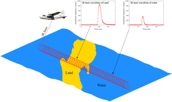
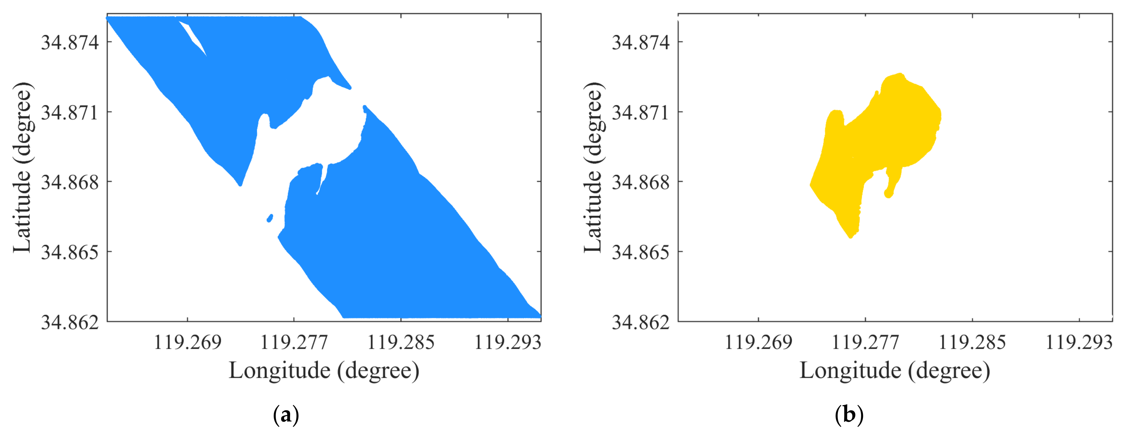
2.1. Research Area and Data Acquisition

The effectiveness of the proposed method is verified by conducting a practical ALB measurement using Optech CZMIL in the coastal waters of Qinshan Island, Jiangsu Province, China on 27 December 2014. Qinshan Island is a non-resident island in the Yellow Sea of China. A wide intertidal zone with white sand or dark mud exists around the island. Bared earth, low vegetation, and tall vegetation exist in the interior of the island.

Table 1. Primary technical parameters of CZMIL.

Parameter	Value
Flight altitude	400 m (nominal)
Flight velocity	140 kts (nominal)
Laser pulse repetition rate	10 kHz
Scanner frequency	27 Hz
Laser wavelength	IR: 1064 nm; green: 532 nm
Maximum measurable depth	4.2/Kd (bottom power reflectivity > 15%)
Minimum measurable depth	0.15 m
Depth accuracy	(0.32 + (0.013 d)2)½ m, 2σ
Horizontal accuracy	(3.5 + 0.05 d) m, 2σ
Scan angle	20° (circular scan)
Cross-track swath width	294 m (nominal)

shows the primary technical parameters of CZMIL, which uses a circular scanner with a fixed incidence angle of 20° and adopts a collinear and synchronous method to emit IR (1064 nm) and green (532 nm) lasers [29,30,31]. The recommended laser pulse repetition rate and scanner frequency for CZMIL are 10 kHz and 27 Hz, respectively [31]. A total of 1,011,132 IR laser waveforms collected in the IR channel of CZMIL and the corresponding 1,011,132 points obtained with IR laser are extracted from raw CZMIL binary files within the research area. Figure 1 shows the position and hill-shaded relief figures of Qinshan Island, which are constructed using 3D point clouds derived with CZMIL. The track lines and flight directions of the three strips (C14, C15, and C16) are represented by black lines with arrows.

The optical properties of water and land are different. Different optical reactions occur when an IR laser arrives at the surface of water and land and result in significant differences in laser pulse waveforms. Figure 2a,b show the typical IR waveforms of water and land collected with Optech CZMIL from with 192 samples, respectively. The amplitude of a land waveform is much larger than that of a water waveform; thus, the amplitude of an IR waveform can be used in identifying water and land waveforms. However, other IR waveform features have not been verified through experimental analysis. Furthermore, special laser waveforms occur in coastal areas with complex environments and result in mislabeled water and land waveforms. Therefore, an optimal feature for water–land discrimination using IR laser should be determined by comparing different features, and mislabeled water–land waveforms should be corrected.

2.2. Feature Selection

The performance of a water–land discrimination method using a single waveform feature and a combination of different features are evaluated and compared.

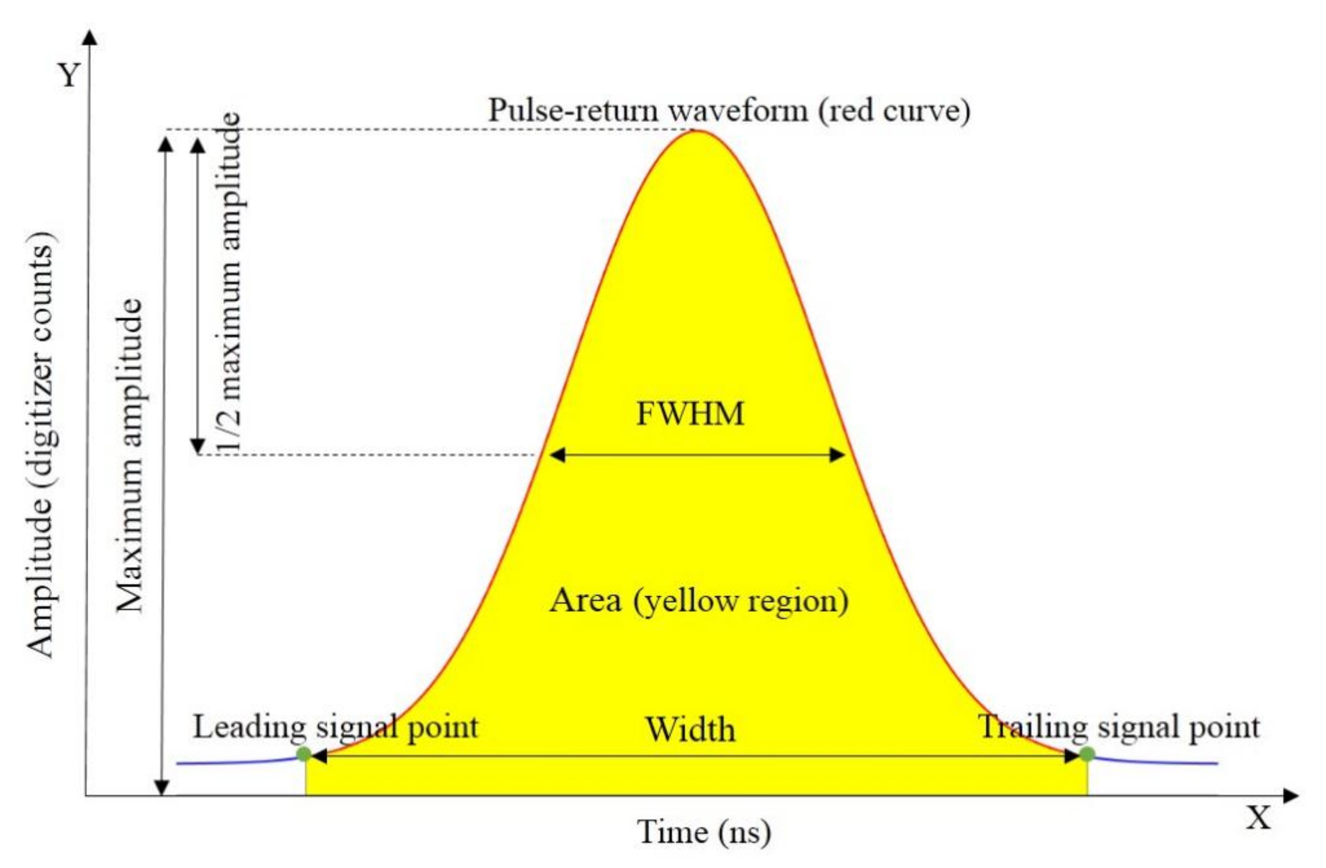
2.2.1. Single Waveform Feature

Apart from waveform amplitudes, other waveform features can be extracted from raw IR laser waveforms. Verifying the effectiveness of water–land discrimination methods using other waveform features is necessary. In Figure 3, features such as amplitude, full width at half maximum (FWHM), area, and width are separately extracted from raw IR laser waveforms and used in verifying their effectiveness in water–land discrimination.

Waveform amplitudes are extracted from an IR laser waveform as follows: let m IR laser full-waveforms be Y = {y₁, y₂, …, y_i, …, y_m}, where y_i is the ith IR full waveform and i ranges from 1 to m. Each full waveform has n samples, that is, y_i = {x₁, x₂, …, x_j, …, x_n}, where x_j is the amplitude of the jth sample in the ith IR full waveform and j ranges from 1 to n. The maximum amplitude of the ith IR full waveform A_i can be extracted according to the following formula:

$$A_i=\max \left(x_i^1,x_i^2,\dots , x_i^j,\dots ,x_i^n\right)$$

(1)

where x^j_i is the amplitude of the jth sample in the ith IR full waveform.

FWHM is the width of waveform at half of amplitude, that is, the time interval between two points on the y-axis, which are half the maximum amplitude, as shown in Figure 3. The FWHM can be calculated with the following formula:

$$FWHM=T_2-T_1$$

(2)

where T₁ and T₂ are the times of the leading and trailing points with half of the maximum amplitude, respectively.

Waveform area is the integral of the pulse return amplitude with respect to time. However, noise inevitably exists in raw IR full waveforms because of the influence of ALB electronics and the environment [32]. A raw full waveform is the sum of pulse-return signal and noise, and noise affects the accuracy of area extraction. Therefore, waveform separation is necessary before feature extraction. Waveform separation can be performed according to Zhao’s separation method [32] for the separation of the pulse-return waveform from a raw full waveform. After waveform separation, the area of the pulse-return waveform can be calculated as follows:

$$S={{\displaystyle \int }}_{t_1}^{t_2}y\left(t\right) dt$$

(3)

where t₁ and t₂ are the times of the leading and trailing edge points of the pulse-return waveform, respectively, and y(t) is the waveform intensity at time t.

Waveform width is the time interval between the leading and the trailing edge points of a pulse-return waveform separated by waveform separation. Width can be calculated by subtracting the leading-edge time from the trailing-edge time of the pulse-return waveform.

2.2.2. Combination of Waveform Features

Whether the performance of water–land discrimination can be improved by using a combination of waveform features with respect to single features needs to be verified. Single waveform features are combined to form different combinations of waveform features.

A reference water–land interface derived from 3D point clouds [11] is used in forming a confusion matrix and calculating the overall accuracy of water–land discrimination using different waveform features. In

Table 2. Confusion matrix for water–land discrimination.

	Water (Reference Label)	Land (Reference Label)
Water (discriminated label)	TN	FN
Land (discriminated label)	FP	TP

, the confusion matrix is derived by comparing discriminated labels (column) against reference ones (row). Diagonal elements in the confusion matrix represent the number of laser measurements in which the discriminated label is the same as the reference label, whereas off-diagonal elements are those that are mislabeled. The overall accuracy OA can be calculated by the following formula:

$$OA=\frac{TP+TN}{TP+FP+TN+FN}$$

(4)

where a true positive (TP) decision is such that a land waveform is assigned to land, a false positive (FP) decision is such that a water waveform is assigned to land, a true negative (TN) decision is such that a water waveform is assigned to water, and a false negative (FN) decision is such that land waveform is assigned to water. OA is used to evaluate the performance of water–land discrimination using different features. The larger OA is, the better the water–land discrimination will be. Thus, the optimal feature for water–land discrimination using IR laser can be determined by OA comparison.

2.3. Dual-Clustering Method for Mislabeled Waveform Correction

Zhao et al. [12] summarized special IR waveforms as follows. First, the IR laser waveforms of bubble-entrained water are mislabeled as land. The strong reflection of an IR laser is due to bubble-entrained water, which enables special IR laser waveforms to achieve amplitudes close to those of the typical IR laser waveforms of land [9]. These special IR laser waveforms of bubble-entrained water are incorrectly labeled as land when the amplitude of an IR waveform is applied. Second, the IR laser waveforms of special land topography are mislabeled as water. Land topography causes the amplitudes of some IR laser waveforms of land to be similar to those of water [12]. These special IR laser waveforms of land are incorrectly labeled as water.

The accuracy of water–land discrimination can be improved by correcting mislabeled waveforms. In reality, water–land interface is obvious and shows spatial continuity. Correctly labeled waveforms appear as aggregated point clouds with high densities in spatial distribution. By contrast, mislabeled waveforms may be single or sparse points and with low densities in spatial distribution, and special mislabeled waveforms induced by complex environments are typical isolated and discrete points with respect to correctly labeled waveforms. Thus, mislabeled waveforms can be corrected if the spatial information of corresponding laser spot centers are considered. K-means clustering is first used to discriminate water/land waveforms through waveform feature clustering. Then, DBSCAN clustering is used to correct mislabeled waveforms by clustering the positions of laser spot centers.

2.3.1. K-Means Clustering

K-means is a classic clustering algorithm based on distance and has low complexity and a good clustering effect. This algorithm can hold better scalability and high efficiency when dealing with large datasets [33,34]. Thus, this study uses the K-means clustering algorithm to cluster water and land waveforms on the basis of waveform amplitudes. In K-means clustering, given a dataset X = {x₁, x₂,…, x_i,…, x_n}, K-means divides the dataset X into k clusters C = {C₁, C₂, …, C_j, …, C_k} by minimizing the squared distance between discrete points and their nearest centroids [35].

$${\displaystyle \sum }_{j=1}^k{\displaystyle \sum }_{i\in C_j}{\parallel X_i-{\mu }_j\parallel }^2$$

(5)

where ∥*∥ denotes the Euclidian distance between each discrete point X_i and centroid of the cluster μ_j calculated by the average of C_j. The number of clusters k for water–land waveform clustering is set to two, namely, water and land. The specific steps of the K-means algorithm for water–land waveform clustering are presented as follows:

Step 1:

Randomly select two points from X as the initial centroids of C₁ and C₂.

Step 2:

Calculate the Euclidean distance d_j = ∥x_i−μ_j∥ between point x_i and centroids μ₁ and μ₂ and assign point x_i to the nearest cluster.

Step 3:

Recalculate the centroids of all clusters using the reassigned points.

Step 4:

Repeat Steps 2 and 3 until μ₁ and μ₂ are stable.

2.3.2. DBSCAN Clustering

DBSCAN is significantly effective in discovering clusters of arbitrary shapes based on the density of data and divides the spatial database into clusters with different densities [36]. Given that DBSCAN can effectively identify outliers with low densities, this study uses DBSCAN algorithm to identify isolated and discrete mislabeled waveforms.

Given a dataset D = {x₁, x₂, …, x_i, …, x_m}, several important definitions are used in DBSCAN. In p ∈ D, the epsilon (Eps)-neighborhood of point p includes the subsample set whose distance from p is less than Eps, namely, N_Eps(p) = {q ∈ D|dist(p, q) ≤ Eps). The number of this subsample set is denoted as |N_Eps(p)|. If the Eps-neighborhood of p contains at least a minimum number (MinPts) of points, that is, |N_Eps(p)| ≥ MinPts, then p would be a core point. In terms of p, q ∈ D, if point q is in the Eps-neighborhood of the core point p, then q is directly density-reachable from p. In dataset D, given a chain of points p₁, p₂, …, p_n, where p = p₁, q = p_n, if p_i is directly density-reachable from p_i−1, then q is density-reachable from p. In terms of p and q, if there is a core point o, and p and q are density-reachable from o, then p is density-connected to q. Given D, Eps, and MinPts, the specific algorithm steps of DBSCAN are presented as follows [37,38,39]:

Step 1

Initialize the core point set Ω = ϕ, the number of clusters k = 0, the sample set unvisited Γ = D, and the cluster division C = ϕ.

Step 2

All core points can be found for i = 1, 2, …, m by following the steps:

(1)

The Eps-neighborhood subsample set N_Eps(x_i) of the sample x_i should be determined through distance measurement;

(2)

If the number of samples in the subsample set satisfies |N_Eps(x_i)| ≥ MinPts, sample x_i will be added to the core point set, that is, Ω = Ω ∪ {x_i}.

Step 3

If the core point set Ω is equal to ϕ, then the algorithm would end. Subsequently, the cluster division C = {C₁, C₂, …, C_k}. Otherwise go to step 4.

Step 4

A core point o needs to be randomly selected from the core point set Ω. Then, the current core point queue Ω_cur = {o}, the serial number k = k + 1, and the current cluster sample set C_k = {o}. The data set unvisited Γ is updated to Γ−{o}.

Step 5

If the current core point queue Ω_cur is ϕ, cluster C would be {C₁, C₂, …, C_k} and the core point set Ω would be Ω−C_k. Then, go to Step 3. Otherwise, the core point set Ω would be Ω−C_k.

Step 6

A core point o’ is taken from the current core point queue Ω_cur. Then, all Eps-neighborhood subsample sets N_Eps(o’) can be found through the Eps-neighborhood distance threshold Eps. Let Δ equal to N_Eps (o’) ∩ Γ. C_k updates to C_k ∪ Δ, Γ updates to Γ−Δ, and Ω_cur updates to Ω_cur ∪ (Δ ∩ Ω)−o’. Then, go to step 5.

2.4. Reference Water–Land Interface

A reference water–land interface is used in evaluating the effectiveness of different waveform features and the clustering method. In situ measurements (such as GNSS-RTK measurements) or satellite imagery [40] can be used as references. Simultaneous GNSS-RTK measurements during ALB measurements can generate accurate water–land interfaces but is costly, time consuming, and dangerous in certain cases. The acquisition time of a satellite image and ALB data may not be entirely synchronized. Water–land interfaces are changing because of the effects of ocean tides and waves. Furthermore, water–land interfaces in satellite images are fuzzy in areas with muddy and sand beaches. Therefore, water–land interfaces derived from satellite images may be inconsistent with the real ones when ALB measurement is carried out. Land elevations are higher than water surface elevations; thus, 3D point clouds can be used in discriminating between water and land [11,12]. Furthermore, water–land interfaces derived using 3D point clouds are theoretically consistent with those derived with IR laser waveforms because both interfaces reflect the water–land interface when ALB measurement is carried out. Precise water–land interfaces derived from 3D point clouds [11] are used as reference for the evaluation of different waveform features and clustering methods.

2.5. Flowchart of the Proposed Water–Land Discrimination Procedure

The flowchart of a water–land discrimination method using IR laser waveforms is shown in Figure 4. First, the IR laser waveforms of airborne LiDAR are extracted from raw ALB data files, and waveform separation is performed for the division of laser waveform into pulse-return and non-pulse-return waveforms. Second, the waveform feature selection method described in Section 2.2 is carried out for the selection of the optimal waveform feature. Finally, the dual-clustering method is performed for discrimination between water and land waveforms. Specifically, K-means clustering is used in clustering waveform amplitude for the generation of rough water and land waveforms. Then, DBSCAN is utilized for the identification and correction of mislabeled waveforms.

3. Results

3.1. Optimal Feature Selection

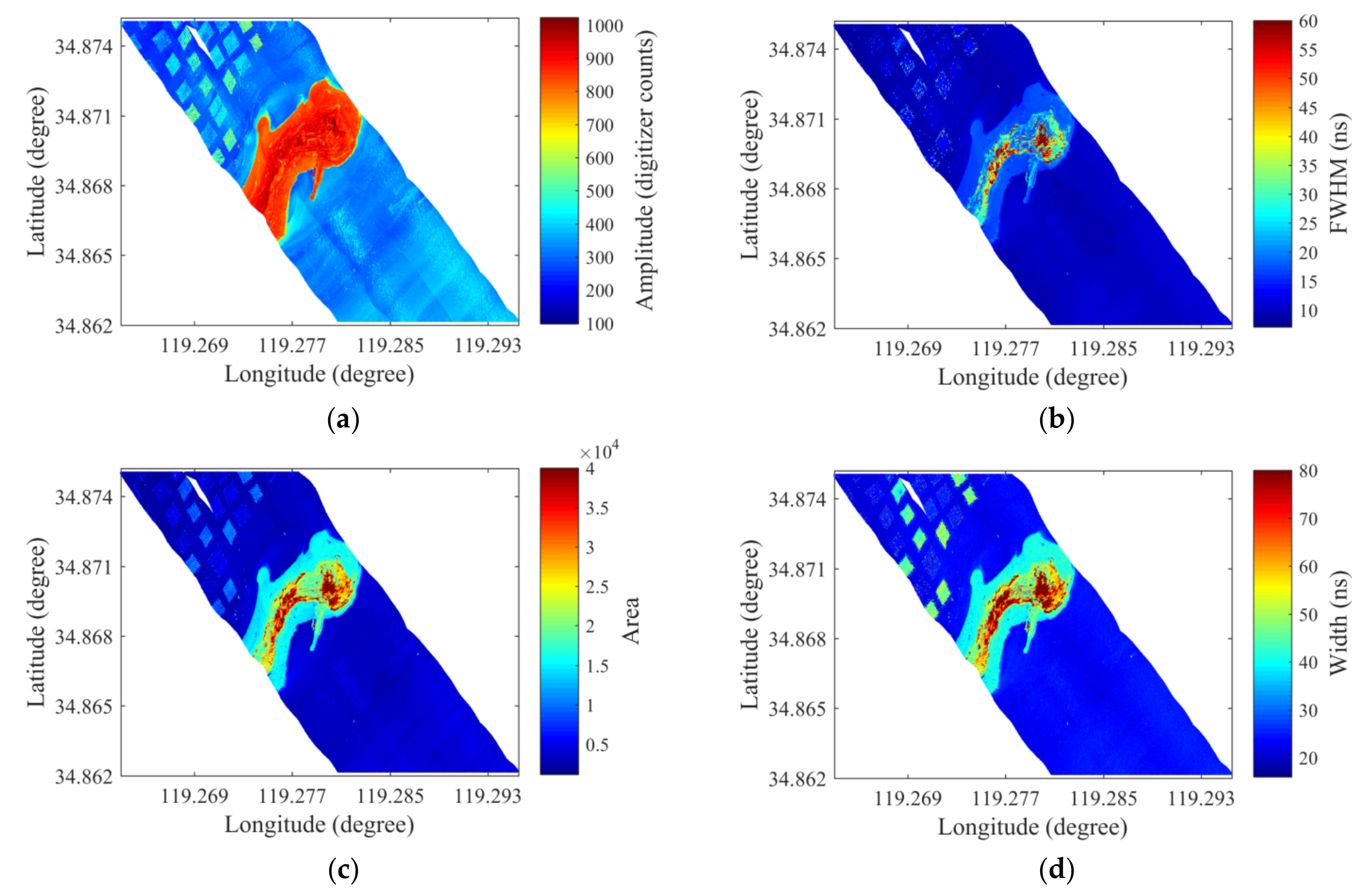
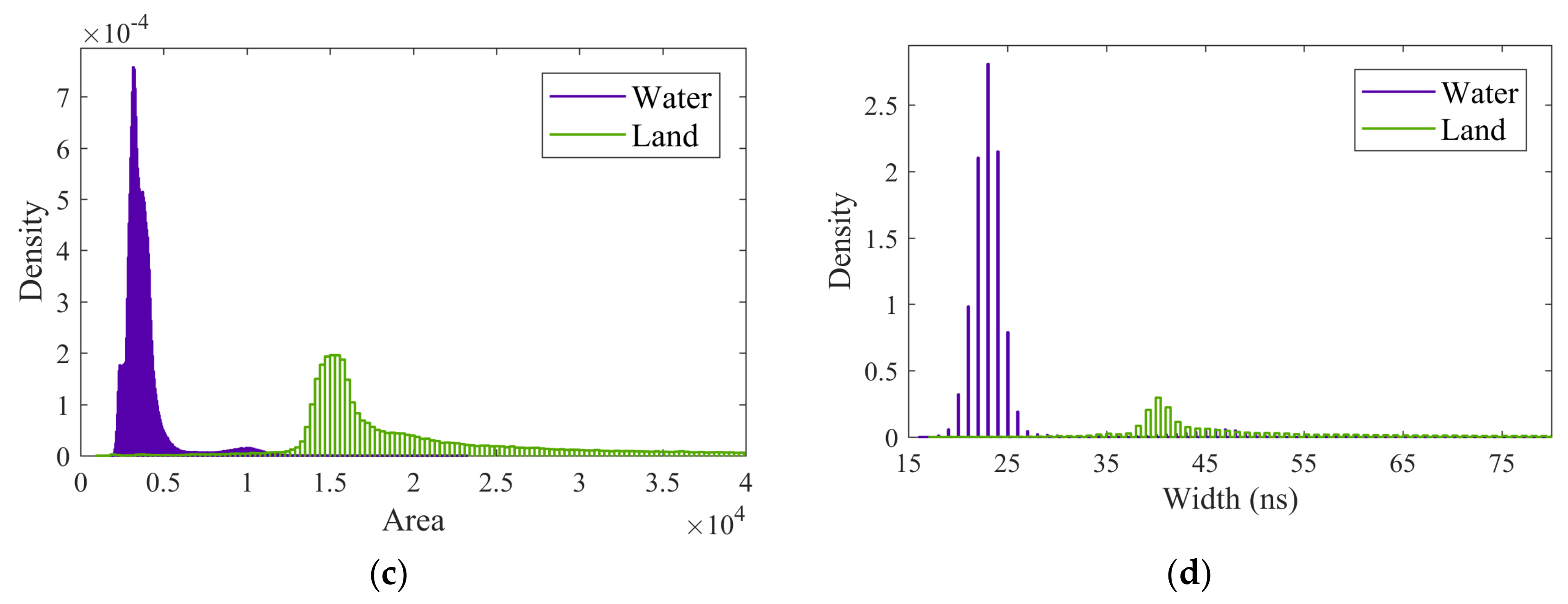
3.1.1. Single Waveform Feature

A raw IR waveform comprises pulse-return and non-pulse-return waveforms. Waveform separation needs to be conducted to reduce the influence of non-pulse-return waveforms on the extraction of the waveform features of pulse-return waveforms. Therefore, waveform separation is necessary before feature extraction. A total of 1,011,132 IR waveforms in the research area are separated into pulse-return and non-pulse-return waveforms according to Zhao’s waveform separation algorithm [32]. Figure 5a,b show the pulse-return and non-pulse-return waveforms separated from a typical IR full waveform, respectively. Then, waveform features such as amplitude, FWHM, area, and width are separately extracted from the pulse-return waveforms according to the method described in Section 2.2.1. Figure 6a–d show the spatial distributions of amplitude, FWHM, area, and width of IR laser waveforms, respectively.

Figure 7a–d show the probability density functions (PDFs) of water/land waveform features (i.e., amplitude, FWHM, area, and width). As shown in Figure 7, the waveform features of water and land are remarkably different, thus further verifying the feasibility of water–land discrimination using IR waveforms. Amplitude, FWHM, area, and width are used to conduct water–land discrimination based on K-means clustering. With the water–land interface derived by 3D point clouds as reference, the confusion matrices similar to those in Table 2 and the overall accuracy of water–land discrimination using different features are shown in

Table 3. Results of water–land discrimination using single features.

Feature	Confusion Matrix			Overall Accuracy
		Reference Water	Reference Land
Amplitude	Discriminated water	839,274	1826	99.48%
	Discriminated land	3416	166,616
FWHM	Discriminated water	840,597	136,299	86.31%
	Discriminated land	2093	32,143
Area	Discriminated water	841,276	5139	99.35%
	Discriminated land	1414	163,303
Width	Discriminated water	802,969	9769	95.11%
	Discriminated land	39,721	158,673

. The confusion matrix and overall accuracy indicate the performance of different features for water–land discrimination. The greater the number of samples correctly identified, the higher the overall accuracy, and the higher the consistence of the discriminated water–land categories with the reference categories.

The spatial distributions of the mislabeled waveforms using amplitude, FWHM, area, and width based on K-means clustering are shown in Figure 8a–d, respectively. In terms of amplitude, 3416 water waveforms are mislabeled as land waveforms, and 1826 land waveforms are mislabeled as water waveforms. The mislabeled water waveforms are induced by the special land topography [12]. The mislabeled land waveforms are induced by bubble-entrained water [9], aquaculture rafts, and a mix of land and water in the laser spot located at the water–land interface. In terms of the FWHM, 136,299 land waveforms are mislabeled as water waveforms, and 2093 water waveforms are mislabeled as land waveforms. The FWHM centroids of the water and land waveforms are 11.4 and 43.2, respectively. FWHM is not influenced by the strong reflection of bubble-entrained water because it reflects the differences in water and land waveforms in the time dimension and not in terms of amplitude. However, many land waveforms are mislabeled as water waveforms, and waveforms reflected from aquaculture rafts are mislabeled as land waveforms because the FWHM values of water and land waveforms are close. With regard to the area, 5139 land waveforms are mislabeled as water waveforms, and 1414 water waveforms are mislabeled as land waveforms. The area centroids of the water and land waveforms are 3800 and 20,000, respectively. The area can reflect the differences in water and land waveforms not only in the time dimension, but also in amplitude. Similar to FWHM, area is rarely influenced by the strong reflection of bubble-entrained water. Nevertheless, many aquaculture raft waveforms are mislabeled as land, and land waveforms are mislabeled as water. In terms of width, 9769 land waveforms are mislabeled as water waveforms, and 39,721 water waveforms are mislabeled as land waveforms. The centroids of the waveform width of water and land waveforms are 23.1 and 49.1, respectively. Similar to FWHM, waveform width reflects the difference in water and land waveforms in the time dimension. Width can better reflect the differences in water and land waveforms than FWHM. However, width is significantly influenced by aquaculture rafts.

Figure 9 shows the typical IR waveforms reflected from aquaculture rafts, water, and land collected by CZMIL. The orange, green, and blue curves represent the waveforms reflected from aquaculture rafts, water, and land, respectively. In Figure 10, the feature values (amplitude, FWHM, area, and width) of typical land waveforms are greater than those of typical water waveforms. Typical ALB systems use a Gaussian temporal and spatial energy distribution [41]. Along the emission direction of the laser, the laser energy presents a Gaussian distribution. The energy distribution across the emission direction is also Gaussian because of the divergence of the laser beam [42]. The closer the position to the central laser ray is, the stronger the laser energy is. Pulse spot size on the water surface is typically 2–3 m [41]. The width and amplitude of waveforms reflected from water are smaller than those reflected from land because of the strong absorption of laser energy by the water surface. No light photon is reflected from the verge of the laser spot on the water surface. The waveforms reflected from aquaculture rafts floating above the water surface have a larger width than those reflected from water, representing the superposition of the waveforms of aquaculture rafts and water. Aquaculture rafts are easily mislabeled as land, and they exert a significant influence on water–land discrimination using FWHM, area, or width. Aquaculture rafts also affect water–land discrimination based on amplitude, but the effect is not as great as that based on FWHM, area, or width.

In summary, water–land discrimination using FWHM, area, or width is rarely influenced by the strong reflection from bubble-entrained water, but it is highly influenced by aquaculture rafts. The results in Table 3 indicate that waveform amplitude has the best performance among the researched features for water–land discrimination in waters with aquaculture rafts.

3.1.2. Combination of Waveform Features

An experimental analysis was conducted to verify whether the performance of water–land discrimination can be improved by using the combination of waveform features. Waveform amplitude is combined with other waveform features to form five new combined features, namely, a combination of amplitude and FWHM; a combination of amplitude and area; a combination of amplitude and width; a combination of amplitude, FWHM, area, and width; and a combination of amplitude, FWHM, area, and width after PCA reduction. Then, these combined features are evaluated by comparing the overall accuracy of water–land discrimination. Water–land discrimination is carried out using amplitude and five combined features through K-means clustering. The overall accuracy of water–land discrimination using different combined features is calculated and shown in

Table 4. Results of water–land discrimination using combined features.

Feature	Confusion Matrix			Overall Accuracy
		Reference Water	Reference Land
Amplitude and FWHM	Discriminated water	839,274	1826	99.48%
	Discriminated land	3416	166,616
Amplitude and area	Discriminated water	841,275	5130	99.35%
	Discriminated land	1415	163,312
Amplitude and width	Discriminated water	839,219	1826	99.48%
	Discriminated land	3471	166,616
Combination of amplitude, FWHM, area, and width	Discriminated water	841,275	5130	99.35%
	Discriminated land	1415	163,312
Combination of amplitude, FWHM, area, and width after PCA reduction	Discriminated water	841,276	5129	99.35%
	Discriminated land	1414	163,313

. In Table 4, the overall accuracy of water–land discrimination using combined features does not improve, but reduces, compared with that using waveform amplitude. Therefore, waveform amplitude is the optimal feature for water–land classification using IR laser waveforms among the researched features in this study.

3.2. Dual-Clustering Method

Waveform amplitudes are used as features for dual clustering. Figure 11 shows the amplitude distribution of 1,011,132 IR laser waveforms, and the pulse number is the abscissa. The laser pulses in the green, red, and yellow regions represent typical land, aquaculture rafts, and water, respectively. The aquaculture rafts are striped wooden structures floating on the water surface. The amplitude distribution of the laser waveforms reflects the environmental changes along the strip, namely, water, land, and aquaculture rafts. The laser waveforms of aquaculture rafts are the mixed waveforms reflected from aquaculture rafts and water because of the large laser spot. The waveform amplitude of the aquaculture raft is between the amplitudes of water and land.

3.2.1. K-Means Clustering

The amplitudes of the 1,011,132 IR waveforms are clustered through K-means clustering according to Section 2.3.1. The amplitude centroids of water and land waveforms are 331 and 851.2, respectively. These values indicate that the difference between the amplitudes of water and land is significant. Figure 12a,b show the spot center positions of land and water IR waveforms labeled through K-means clustering, respectively. Land and water waveforms are effectively discriminated with a clear water–land interface. However, numerous mislabeled waveforms exist in the water and land areas. In Figure 12a, numerous scattered waveforms exist in the island areas. These IR waveforms can be divided into two types. The first type includes mislabeled water waveforms induced by complex land topography. The other one includes the correctly identified water waveforms of ponds or reservoirs in islands. The waveforms of ponds or reservoirs can be verified using IR laser amplitudes and elevations, given that they are aggregation points with low waveform amplitudes and small elevation fluctuations. In Figure 12b, numerous laser points exist in an ocean area. These points are mislabeled as land waveforms because of the presence of bubble-entrained water and wooden aquaculture rafts floating on the ocean surface. IR waveform amplitudes reflected from bubble-entrained water or wooden aquaculture rafts are as large as those reflected from land. These mislabeled waveforms reduce the accuracy of water–land discrimination. The results further indicate the necessity of mislabeled waveform correction. The spatial densities of mislabeled waveforms that can be regarded as noise are lower compared with the densities of correctly labeled water and land waveforms. The spatial distance between the correctly labeled and mislabeled waveforms is significant. Therefore, the spatial distribution information can be used in correcting the mislabeled waveforms.

3.2.2. DBSCAN Clustering

DBSCAN clustering is used in identifying and correcting mislabeled water and land waveforms by clustering the positions of laser spots. The water and land waveforms derived through K-Means clustering are clustered again through DBSCAN according to the positions of laser spots. The criteria of DBSCAN clustering for this study are the premises that the integrity of water and land areas can be ensured, mislabeled waveforms can be identified, and inland water bodies, such as ponds or reservoirs, can be retained. The parameter settings of Eps and MinPts in DBSCAN are 0.0001 and 4, respectively, on the basis of experimental analysis. Figure 13 shows the DBSCAN results of water and land waveforms. Mislabeled water and land waveforms are successfully identified with DBSCAN. As shown in the island area in Figure 13a, mislabeled water waveforms induced by complex land topography are identified and represented by the red color. Water waveforms reflected from ponds in islands are maintained. In Figure 13b, the mislabeled land waveforms in ocean areas are successfully identified with DBSCAN. The mislabeled water and land waveforms identified with DBSCAN are corrected into land and water waveforms, respectively. The laser spot positions of the final water and land waveforms are shown in Figure 14. The results show that DBSCAN effectively identifies the mislabeled waveforms (noise), and water–land interfaces are clear and smooth.

The water and land waveforms determined through K-means clustering and dual clustering and by using the pulse number as the abscissa are shown in Figure 15a,b, respectively. Traditional water–land discrimination using K-means clustering only considers waveform features, and a clear dividing line exists between the amplitudes of water and land waveforms, resulting in numerous mislabeled waveforms. By contrast, dual clustering not only considers the waveform amplitude but also the position of the laser spot. K-means clustering is used in clustering waveform amplitudes for the generation of rough water and land waveforms, and DBSCAN is utilized for the identification and correction of mislabeled waveforms through the clustering of spot positions. The dual-clustering method proposed in this study uses IR waveform amplitudes to distinguish land from water and the positions of laser spots to correct mislabeled waveforms. Hence, mislabeled water waveforms with amplitudes close to those of land waveforms are corrected to land waveforms, and mislabeled land waveforms with amplitudes close to those of land waveforms are corrected to water waveforms. The influence of environmental factors on the water–land discrimination is reduced, and the accuracy of water–land discrimination is improved.

3.2.3. Accuracy Analysis

The water–land interface derived by 3D point cloud is used as a reference for the evaluation and comparison of the performance of K-means clustering and dual-clustering methods.

Table 5. Results of water–land discrimination using two clustering methods.

Method	Confusion Matrix			Overall Accuracy
		Reference Water	Reference Land
K-means	Discriminated water	839,274	1826	99.48%
	Discriminated land	3416	166,616
Dual clustering	Discriminated water	841,615	1659	99.73%
	Discriminated land	1075	166,783

shows the confusion matrices of K-means clustering and dual clustering using IR waveform amplitude, which are used in calculating their respective overall accuracy rates. The overall accuracy rates of K-means clustering and dual clustering are 99.482% and 99.730%, respectively. The dual clustering corrects a total of 2508 mislabeled IR waveforms, including 167 mislabeled water waveforms and 2341 mislabeled land waveforms, compared with K-means clustering. The proposed dual-clustering method can correct mislabeled water or land waveforms and reduce the number of mislabeled waveforms by 48% with respect to the number obtained through traditional K-means clustering. The mislabeled waveform correction improves the overall accuracy of water–land discrimination.

4. Discussion

4.1. Influencing Factors for Water–Land Discrimination

Feature extraction, feature selection, and clustering method are the three main factors that influence the performance of water–land discrimination using laser waveforms. The quality of waveform features can be controlled by improving the accuracy of feature extraction. Waveform separation can reduce the influence of non-pulse-return waveform on the feature extraction of pulse-return waveform. The performance of water–land discrimination is highly influenced by the waveform feature. Feature selection should be conducted in the selection of optimal features, and the performance of different waveform features is compared. Waveform amplitude is suggested to be the optimal feature for water–land discrimination using IR laser waveforms by experimental analysis in this study. The clustering method is the third influencing factor. The proposed dual-clustering method can correct the mislabeled water and land waveforms and improve the overall accuracy of water–land discrimination.

4.2. Detection of Aquaculture Rafts Using Waveform Width

Research suggests that aquaculture rafts provide favorable substrates for the microscopic propagules of Ulva prolifera. Aquaculture rafts play an important role in offering attachment conditions for the early formation of green tides [43]. The monitoring of aquaculture rafts using satellite imagery is highly limited by environmental factors, such as haze, clouds, illumination conditions, and image resolution. Moreover, it cannot provide structural information in vertical directions. As analyzed in Section 3.1.1, water–land discrimination using waveform width is not influenced by the strong reflection of bubble-entrained water, but it is highly influenced by aquaculture rafts. The sensitivity of waveform width to aquaculture rafts is not beneficial for water–land discrimination, but it provides a possible approach to the detection and extraction of aquaculture rafts. Figure 16a shows the spatial distributions of aquaculture rafts detected using waveform width. Figure 16b displays the structural information of an aquaculture raft in the vertical direction. The spatial distributions and structural information in the vertical direction of aquaculture rafts can be detected with high accuracy and resolution by using waveform width and the point clouds of airborne infrared laser.

4.3. Applications

The proposed method using IR laser waveforms is suitable for airborne LiDAR systems with IR lasers, that is, airborne topographic LiDAR systems or integrated IR and green ALB systems, and is not applicable to green-only ALB systems, which have no additional IR lasers. Water–land discrimination using green laser waveforms is low because the green laser waveform is highly influenced by the merge effect in very shallow waters [12]. More studies should be carried out to improve the accuracy of water–land discrimination using green laser waveforms. The results of water–land discrimination using IR laser waveforms in this study can be used as an exact external reference for the evaluation of the performance of water–land discrimination using green laser waveforms.

5. Conclusions

This study verifies the performance of the different features of IR waveforms and proposes a dual-clustering method to correct mislabeled waveforms for water–land discrimination using airborne infrared LiDAR.

(1)

The performance of water–land discrimination using single waveform features and combinations of waveform features are evaluated and compared through experimental analysis. The overall accuracy rates of water–land discrimination using amplitude; FWHM; area; width; a combination of amplitude and FWHM; a combination of amplitude and area; a combination of amplitude and width; a combination of amplitude, FWHM, area, and width; and a combination of amplitude, FWHM, area, and width after PCA reduction based on K-means clustering are 99.482%, 86.313%, 99.352%, 95.105%, 99.482%, 99.353%, 99.476%, 99.353%, and 99.353%, respectively. The results show that waveform amplitude is the optimal feature for water–land discrimination using IR laser waveforms.

(2)

Dual-clustering has two levels. The first level removes outliers in the waveform amplitudes. The second level removes geographic outliers to correct the mislabeled waveforms derived by the first level. The proposed dual-clustering method can correct mislabeled water or land waveforms and reduce the number of mislabeled waveforms by 48% with respect to the number obtained through traditional K-means clustering. Water–land discrimination using IR waveform amplitude and the proposed dual-clustering method can reach an overall accuracy of 99.730%. The proposed dual-clustering method can correct and reduce mislabeled waveforms with respect to the traditional feature clustering methods.

Water–land discrimination using IR laser waveform amplitudes and the proposed dual-clustering method is robust and highly accurate, has a high resolution, and is capable of automation. Hence, its use in coastal and inland waters is recommended.

References

1. Guenther, G.C. Airborne Laser Hydrography: System Design and Performance Factors; NOAA Professional Paper Series; NOAA: Washington, DC, USA, 1985; pp. 1–385. [Google Scholar]
2. Guenther, G.C.; Cunningham, A.G.; LaRocque, P.E.; Reid, D.J. Meeting the accuracy challenge in airborne Lidar bathymetry. In Proceedings of the 20th EARSeL Symposium: Workshop on Lidar Remote Sensing of Land and Sea, Dresden, Germany, 16–17 June 2000; pp. 1–27. [Google Scholar]
3. Hilldale, R.C.; Raff, D. Assessing the ability of airborne LiDAR to map river bathymetry. Earth Surf. Process. Landf. 2008, 33, 773–783. [Google Scholar] [CrossRef]
4. Kinzel, P.J.; Legleiter, C.J.; Nelson, J.M. Mapping river bathymetry with a small footprint green lidar: Applications and challenges. J. Am. Water Resour. Assoc. 2013, 49, 183–204. [Google Scholar] [CrossRef]
5. Saylam, K.; Hupp, J.R.; Averett, A.R.; Gutelius, W.F.; Gelhar, B.W. Airborne lidar bathymetry: Assessing quality assurance and quality control methods with Leica Chiroptera examples. Int. J. Remote. Sens. 2018, 39, 2518–2542. [Google Scholar] [CrossRef]
6. Allouis, T.; Bailly, J.-S.; Pastol, Y.; Le Roux, C. Comparison of LiDAR waveform processing methods for very shallow water bathymetry using Raman, near-infrared and green signals. Earth Surf. Process. Landf. 2010, 35, 640–650. [Google Scholar] [CrossRef]
7. Mandlburger, G.; Pfennigbauer, M.; Pfeifer, N. Analyzing near water surface penetration in laser bathymetry—A case study at the River Pielach. ISPRS Ann. Photogramm. Remote. Sens. Spat. Inf. Sci. 2013, II-5/W2, 175–180. [Google Scholar] [CrossRef] [Green Version]
8. Zhao, J.; Zhao, X.; Zhang, H.; Zhou, F. Shallow Water Measurements Using a Single Green Laser Corrected by Building a Near Water Surface Penetration Model. Remote Sens. 2017, 9, 426. [Google Scholar] [CrossRef] [Green Version]
9. Pe’Eri, S.; Morgan, L.V.; Philpot, W.D.; Armstrong, A.A. Land-Water Interface Resolved from Airborne LIDAR Bathymetry (ALB) Waveforms. J. Coast. Res. 2011, 62, 75–85. [Google Scholar] [CrossRef]
10. Collin, A.; Long, B.; Archambault, P. Merging land-marine realms: Spatial patterns of seamless coastal habitats using a multispectral LiDAR. Remote. Sens. Environ. 2012, 123, 390–399. [Google Scholar] [CrossRef]
11. Zhao, X.; Wang, X.; Zhao, J.; Zhou, F. Water–land classifification using three-dimensional point cloud data of airborne LiDAR bathymetry based on elevation threshold intervals. J. Appl. Remote. Sens. 2019, 13, 034511. [Google Scholar] [CrossRef]
12. Zhao, X.; Wang, X.; Zhao, J.; Zhou, F. An Improved Water–land Discriminator Using Laser Waveform Amplitude and Point Cloud Elevation of Airborne LiDAR. J. Coast. Res. 2021. [Google Scholar] [CrossRef]
13. Zhao, X.; Zhao, J.; Zhang, H.; Zhou, F. Remote Sensing of Suspended Sediment Concentrations Based on the Waveform Decomposition of Airborne LiDAR Bathymetry. Remote Sens. 2018, 10, 247. [Google Scholar] [CrossRef] [Green Version]
14. Zhao, X.; Zhao, J.; Zhang, H.; Zhou, F. Remote Sensing of Sub-Surface Suspended Sediment Concentration by Using the Range Bias of Green Surface Point of Airborne LiDAR Bathymetry. Remote Sens. 2018, 10, 681. [Google Scholar] [CrossRef] [Green Version]
15. Tulldahl, H.M.; Steinvall, K.O. Simulation of sea surface wave influence on small target detection with airborne laser depth sounding. Appl. Opt. 2004, 43, 2462–2483. [Google Scholar] [CrossRef] [PubMed]
16. Westfeld, P.; Maas, H.-G.; Richter, K.; Weiß, R. Analysis and correction of ocean wave pattern induced systematic coordinate errors in airborne LiDAR bathymetry. ISPRS J. Photogramm. Remote Sens. 2017, 128, 314–325. [Google Scholar] [CrossRef]
17. Xu, W.; Guo, K.; Liu, Y.; Tian, Z.; Tang, Q.; Dong, Z.; Li, J. Refraction error correction of Airborne LiDAR Bathymetry data considering sea surface waves. Int. J. Appl. Earth Obs. Geoinf. 2021, 102, 102402. [Google Scholar] [CrossRef]
18. Guo, K.; Li, Q.; Mao, Q.; Wang, C.; Zhu, J.; Liu, Y.; Xu, W.; Zhang, D.; Wu, A. Errors of Airborne Bathymetry LiDAR Detection Caused by Ocean Waves and Dimension-Based Laser Incidence Correction. Remote Sens. 2021, 13, 1750. [Google Scholar] [CrossRef]
19. Wang, C.-K.; Philpot, W. Using airborne bathymetric lidar to detect bottom type variation in shallow waters. Remote Sens. Environ. 2007, 106, 123–135. [Google Scholar] [CrossRef]
20. Narayanan, R.; Sohn, G.; Kim, H.B.; Miller, J.R. Soft classification of mixed seabed points based on fuzzy clustering analysis using airborne LIDAR bathymetry data. J. Appl. Remote Sens. 2011, 5, 053534. [Google Scholar] [CrossRef]
21. Su, D.; Yang, F.; Ma, Y.; Zhang, K.; Huang, J.; Wang, M. Classification of coral reefs in the south china sea by combining air-borne lidar bathymetry bottom waveforms and bathymetric features. IEEE Trans. Geosci. Remote Sens. 2019, 57, 815–828. [Google Scholar] [CrossRef]
22. Guenther, G.C.; Larocque, P.E.; Lillycrop, W.J. Multiple surface channels in Scanning Hydrographic Operational Airborne Lidar Survey (SHOALS) airborne lidar. In Proceedings of the Ocean Optics XII, Bergen, Norway, 26 October 1994; Volume 2258, pp. 422–430. [Google Scholar]
23. Pe’eri, S.; Philpot, W. Increasing the Existence of Very Shallow-Water LIDAR Measurements Using the Red-Channel Wave-forms. IEEE Trans. Geosci. Remote Sens. 2007, 45, 1217–1223. [Google Scholar] [CrossRef]
24. Cao, B.; Zhu, S.; Qiu, Z.; Cao, B. Water–land classification for LiDAR bathymetric data based on echo waveform characteristics. Hydrographic surveying and charting. Hydrogr. Surv. Chart. 2018, 38, 12–16. [Google Scholar]
25. Qiu, Z.; Cao, B. Water–land classification method for airborne LiDAR bathymetric data. In Proceedings of the China Inertial Technology Society High-end Frontier Special Topics Academic Conference, Beijing, China, 10 December 2017; pp. 328–338. [Google Scholar]
26. Huang, T.; Tao, B.; Mao, Z.; He, Y.; Hu, S.; Wang, C.; Yu, J.; Chen, P. Classification of sea and land waveform based on multi–channel ocean LiDAR. Chin. J. Lasers 2017, 44, 294–303. [Google Scholar]
27. Fuchs, E.; Tuell, G. Conceptual design of the CZMIL data acquisition system (DAS): Integrating a new bathymetric lidar with a commercial spectrometer and metric camera for coastal mapping applications. Proc. SPIE 2010, 7695, 76950U. [Google Scholar] [CrossRef]
28. Zhang, X.; Lewis, M.; Johnson, B. Influence of bubbles on scattering of light in the ocean. Appl. Opt. 1998, 37, 6525–6536. [Google Scholar] [CrossRef] [PubMed]
29. Pierce, J.W.; Fuchs, E.; Nelson, S.; Feygels, V.; Tuell, G. Development of a novel laser system for the CZMIL lidar. Proc. SPIE 2010, 7695, 76950. [Google Scholar] [CrossRef]
30. Payment, A.; Feygels, V.; Fuchs, E. Proposed lidar receiver architecture for the CZMIL system. Proc. SPIE 2010, 7695, 76950. [Google Scholar] [CrossRef]
31. Fuchs, E.; Mathur, A. Utilizing circular scanning in the CZMIL system. Proc. SPIE 2010, 7695, 76950W. [Google Scholar] [CrossRef]
32. Zhao, X.; Liang, G.; Liang, Y.; Zhao, J.; Zhou, F. Background noise reduction for airborne bathymetric full waveforms by cre-ating trend models using Optech CZMIL in the Yellow Sea of China. Appl. Opt. 2020, 59, 11019–11026. [Google Scholar] [CrossRef]
33. Kanungo, T.; Mount, D.M.; Netanyahu, N.S.; Piatko, C.D.; Silverman, R.; Wu, A.Y. A local search approximation algorithm for k-means clustering. Comput. Geom. 2004, 28, 89–112. [Google Scholar] [CrossRef]
34. Abdeyazdan, M. Data clustering based on hybrid K-harmonic means and modifier imperialist competitive algorithm. J. Supercomput. 2013, 68, 574–598. [Google Scholar] [CrossRef]
35. Li, R.; Huang, Y.; Wang, J. Long-term traffic volume prediction based on K-means Gaussian interval type-2 fuzzy sets. IEEE/CAA J. Autom. Sin. 2019, 1–8. [Google Scholar] [CrossRef]
36. Ester, M.; Kriegel, H.P.; Sander, J.; Xu, X. A density-based algorithm for discovering clusters in large spatial databases with noise. AAAI Press 1996, 96, 226–231. [Google Scholar]
37. Cui, H.; Wu, W.; Zhang, Z.; Han, F.; Liu, Z. Clustering and application of grain temperature statistical parameters based on the DBSCAN algorithm. J. Stored Prod. Res. 2021, 93, 101819. [Google Scholar] [CrossRef]
38. Çelik, M.; Dadaşer-Çelik, F.; Dokuz, A.Ş. Anomaly detection in temperature data using DBSCAN algorithm. In Proceedings of the 2011 International Symposium on Innovations in Intelligent Systems and Applications, Istanbul, Turkey, 15–18 June 2011; pp. 91–95. [Google Scholar]
39. Shen, J.; Hao, X.; Liang, Z.; Liu, Y.; Wang, W.; Shao, L. Real-Time Superpixel Segmentation by DBSCAN Clustering Algorithm. IEEE Trans. Image Process. 2016, 25, 5933–5942. [Google Scholar] [CrossRef] [Green Version]
40. Randazzo, G.; Barreca, G.; Cascio, M.; Crupi, A.; Fontana, M.; Gregorio, F.; Lanza, S.; Muzirafuti, A. Analysis of Very High Spatial Resolution Images for Automatic Shoreline Extraction and Satellite-Derived Bathymetry Mapping. Geosciences 2020, 10, 172. [Google Scholar] [CrossRef]
41. Carr, D.A. A Study of the Target Detection Capabilities of an Airborne Lidar Bathymetry System. Ph.D. Thesis, Georgia Institute of Technology, Atlanta, GA, USA, 2013. [Google Scholar]
42. Zhao, X.; Zhao, J.; Wang, X.; Zhou, F. Improved waveform decomposition with bound constraints for green waveforms of airborne LiDAR bathymetry. J. Appl. Remote Sens. 2020, 14, 027502. [Google Scholar] [CrossRef]
43. Geng, H.; Yan, T.; Yu, R.; Zhang, Q.; Kong, F.; Zhou, M. Comparative study on germination of Ulva prolifera spores on different substrates. Oceanol. Limnol. Sin. 2018, 49, 1006–1013. [Google Scholar]
Figure 1. Location and hill-shaded relief figures of the research area.
Remotesensing 13 03628 g001
Figure 2. Typical IR waveforms of (a) water and (b) land.
Remotesensing 13 03628 g002
Figure 3. Features of IR laser waveform.
Remotesensing 13 03628 g003
Figure 4. Flow chart of the proposed dual-clustering method.
Remotesensing 13 03628 g004
Figure 5. (a) Pulse-return and (b) non-pulse-return waveforms of a typical IR full waveform.
Remotesensing 13 03628 g005
Figure 6. Spatial distributions of (a) amplitude, (b) FWHM, (c) area, and (d) width of IR laser waveforms.
Remotesensing 13 03628 g006
Figure 7. PDFs of (a) amplitude, (b) FWHM, (c) area, and (d) width of water–land waveforms.
Remotesensing 13 03628 g007aRemotesensing 13 03628 g007b
Figure 8. Spatial distributions of mislabeled waveforms derived by (a) amplitude, (b) FWHM, (c) area, and (d) width based on K-means clustering.
Remotesensing 13 03628 g008
Figure 9. Typical IR waveforms reflected from aquaculture raft (orange), water (green), and land (blue) collected by CZMIL.
Remotesensing 13 03628 g009
Figure 10. Illustration of IR waveforms reflected from (a) aquaculture rafts, (b) water, and (c) land.
Remotesensing 13 03628 g010
Figure 11. Distribution of waveform amplitudes of water (yellow), aquaculture rafts (red), and land (green) with pulse number as abscissa.
Remotesensing 13 03628 g011
Figure 12. Spot center positions of (a) water and (b) land IR waveforms labeled by K-means clustering.
Remotesensing 13 03628 g012
Figure 13. DBSCAN results of (a) water and (b) land waveforms derived through K-means clustering.
Remotesensing 13 03628 g013
Figure 14. Laser spot positions of final (a) water and (b) land waveforms.
Remotesensing 13 03628 g014
Figure 15. Water/land waveforms derived by (a) K-means and (b) dual clustering.
Remotesensing 13 03628 g015
Figure 16. Structural information in the (a) horizontal and (b) vertical directions.
Remotesensing 13 03628 g016