Technical Note

Global Ocean Studies from CALIOP/CALIPSO by Removing Polarization Crosstalk Effects

1
Science Systems Applications, Inc., Hampton, VA 23666, USA
2
NASA Langley Research Center, Hampton, VA 23681, USA
*
Author to whom correspondence should be addressed.
Remote Sens. 2021, 13(14), 2769; https://doi.org/10.3390/rs13142769
Submission received: 7 June 2021 / Revised: 10 July 2021 / Accepted: 12 July 2021 / Published: 14 July 2021
(This article belongs to the Special Issue Monitoring Aquatic Environments Using LiDAR)

Abstract

:
Recent studies indicate that the Cloud-Aerosol Lidar with Orthogonal Polarization (CALIOP) aboard the Cloud-Aerosol Lidar and Infrared Pathfinder Satellite Observations (CALIPSO) satellite provides valuable information about ocean phytoplankton distributions. CALIOP’s attenuated backscatter coefficients, measured at 532 nm in receiver channels oriented parallel and perpendicular to the laser’s linear polarization plane, are significantly improved in the Version 4 data product. However, due to non-ideal instrument effects, a small fraction of the backscattered optical power polarized parallel to the receiver polarization reference plane is misdirected into the perpendicular channel, and vice versa. This effect, known as polarization crosstalk, typically causes the measured perpendicular signal to be higher than its true value and the measured parallel signal to be lower than its true value. Therefore, the ocean optical properties derived directly from CALIOP’s measured signals will be biased if the polarization crosstalk effect is not taken into account. This paper presents methods that can be used to estimate the CALIOP crosstalk effects from on-orbit measurements. The global ocean depolarization ratios calculated both before and after removing the crosstalk effects are compared. Using CALIOP crosstalk-corrected signals is highly recommended for all ocean subsurface studies.

Graphical Abstract

1. Introduction

The Cloud-Aerosol Lidar and Infrared Pathfinder Satellite Observations (CALIPSO) mission is a pioneering international partnership between NASA and the French Space Agency, CNES [1,2,3]. The CALIPSO mission is entering its 16th year of very successful operation, providing the first decadal dataset of high-resolution atmospheric profiles of aerosols and clouds globally [3], which are critical to earth radiation budget estimation and climate model improvements. The Cloud-Aerosol Lidar with Orthogonal Polarization (CALIOP), a dual-wavelength (532 nm and 1064 nm) polarization sensitive (at 532 nm) elastic backscatter lidar, is the prime payload instrument on the CALIPSO satellite [1]. The main objective of CALIOP is to provide global mapping of the vertical structure of the Earth’s atmosphere [4].
Although CALIOP was not designed for ocean subsurface applications, its measurements over the Earth’s oceans now provide a wealth of unanticipated opportunities for ocean biology and biogeochemistry studies. During the past decade, innovative retrieval methods have been developed to translate CALIOP’s ocean backscattered signals into ocean optical properties such as global phytoplankton distributions [5], total particulate organic carbon (POC) stocks [5,6], particulate backscattering coefficients (bbp, m−1) [7,8,9,10], phytoplankton biomass estimates [11], and depolarization ratios of ocean waters [12,13,14]. These breakthroughs have demonstrated that the satellite lidar era in the oceanography has arrived [15,16,17].
However, non-ideal polarization separation by the optical components in the CALIOP receiver can cause some small fraction of the backscattered optical power polarized parallel to the receiver reference plane to be misdirected into the perpendicular channel, and vice versa [18]. This effect, known as polarization crosstalk, typically causes the measured cross-polarized (i.e., the perpendicular channel, s) attenuated backscatter coefficient ( β s , m−1sr−1) to be higher than its true value and the measured co-polarized (i.e., the parallel channel, p) attenuated backscatter coefficient ( β p , m−1sr−1) to be lower than its true value [19,20].
Because the backscatter signals from beneath the ocean surface are highly attenuated, the relative errors in the CALIOP measured cross-polarized attenuated backscatter coefficient ( β s ,   m e a s u r e d β s ,   t r u e β s ,   t r u e × 100 % ) due to crosstalk can be up to 100% or more for some scenes, which will in turn introduce biases into the subsequently derived ocean optical properties, such as bbp, POC stocks, phytoplankton biomass, etc. (Section 2.3). Consequently, estimates of ocean optical properties derived from CALIOP measurements must take crosstalk into account and the crosstalk artifacts should be removed before retrieving ocean optical properties. Previous CALIOP ocean studies [5,10,11] with crosstalk properly handled should not be questioned. Unfortunately, previous analyses of CALIOP data for ocean studies [7,12,13] ignored the effect of optical crosstalk between the 532 nm parallel and perpendicular channels will have relatively high crosstalk induced errors.
The objectives of this study are to (1) estimate the magnitude of CALIOP’s polarization crosstalk from on-orbit measurements, (2) provide a correction method to remove crosstalk effects on CALIOP measured attenuated backscatter coefficients, and (3) compare the ocean results retrieved before and after applying the crosstalk correction. In Section 2, we describe the methods used to estimate the crosstalk from CALIOP Level 1 (L1) data and develop a straightforward correction function. The global ocean depolarization ratio results before and after crosstalk correction are compared in Section 3. We conclude with a summary of our investigations in Section 4.

2. Methods

The analysis and results presented in this work use CALIOP Version 4.1 (V4) Level 1 (L1) data products [21], in which the calibration of the 532 nm attenuated backscatter coefficients is significantly improved [22,23].
The CALIOP backscatter signal at 532 nm is separated into parallel (p) and perpendicular (s) components by polarization beam splitters (PBS) in the receiver subsystem [1,2]. The crosstalk (CTp2s) represents the fraction of the optical power polarized parallel to the receiver polarization reference plane that is transferred to the perpendicular channel, as follows:
β s , m e a s u r e d ( z ) = β s , t r u e ( z ) + C T p 2 s × β p , t r u e ( z )   and
β p , m e a s u r e d ( z ) = β p , t r u e ( z ) C T p 2 s × β p , t r u e ( z ) .
Here, a fraction ( C T p 2 s ) of β p ,   t r u e is reflected into the perpendicular channel (Equation (1)) and the remainder (1 − C T p 2 s ) of the parallel signal β p ,   t r u e is transmitted into the parallel detector (Equation (2)). The polarization crosstalk from perpendicular channel to parallel channel ( C T s 2 p ) is ignored in Equations (1) and (2) because the contribution of C T s 2 p × β s , t r u e ( z ) to both 532 nm channels is less than 1%, while the contribution of C T p 2 s × β p , t r u e ( z ) to perpendicular channel (Equation (1)) can be as large as 100% or more (Section 2.3) and should be taken into account.

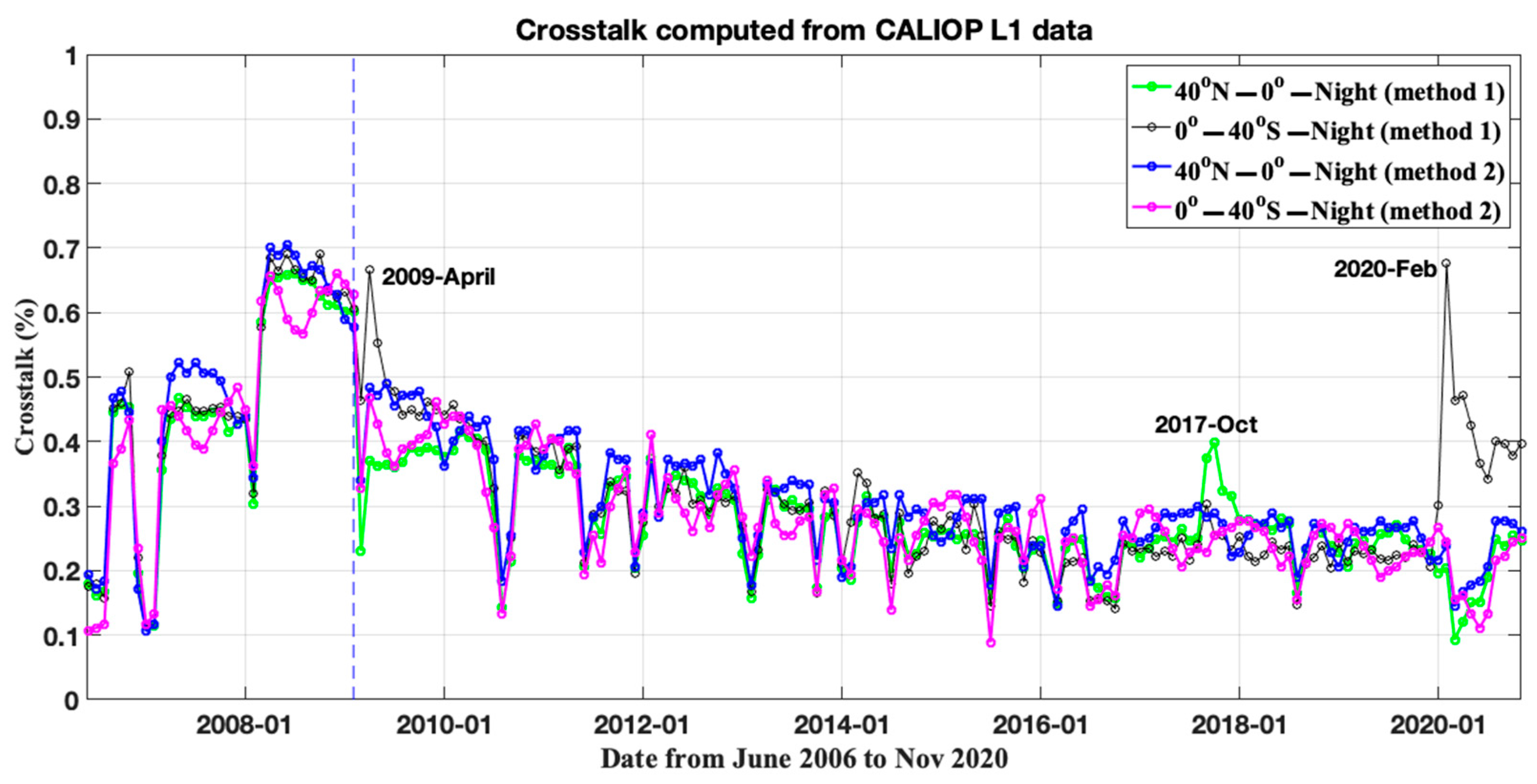
2.1. Crosstalk Estimation from Clear Air Depolarization Ratio (Method 1)

CALIOP clear air depolarization ratio measurements have no particular scientific interest, since the depolarization ratio of clear air is known to be around 0.0035 for the optical filter passbands implemented in the CALIOP receiver. However, they are of interest from an instrument performance standpoint because they allow us to monitor the crosstalk between the parallel and perpendicular channels. For this investigation, the CALIOP measured clear air depolarization ratio ( δ m o l ) is calculated as:
δ m o l = z = 20 k m z = 30 k m β s ,   m e a s u r e d ( z ) / z = 20 k m z = 30 k m β p ,   m e a s u r e d ( z )
i.e., the mean perpendicular attenuated backscatter coefficient divided by the mean parallel attenuated backscatter coefficient, with the means computed over the altitude region from 20 km to 30 km. The signals in this altitude regime consist almost entirely of molecular backscatter. Aerosol scattering is generally negligible, and cloud contributions at these altitudes can be neglected entirely. This calculation excludes the wintertime polar regions, where polar stratospheric clouds may contribute significantly to the signal.
With an ideal beam splitter, δ m o l estimates obtained by using Equation (3) would approximately equal the theoretical value of 0.0035. Absent shot noise and with perfect calibration, these δmol values would exactly equal the theoretical value. The difference between the measured and theoretical molecular depolarization ratios can indicate the level of crosstalk between the two polarization channels. From CALIOP L1 data, which are well calibrated [22,23], the CTp2s can be estimated as (method 1):
C T p 2 s = δ m o l 0.0035 ,
where the measured molecular depolarization ratio ( δ m o l ) is calculated by Equation (3) from L1 nighttime data for two chosen latitude regions, 0° to 40° N and 0° to 40° S, where the South Atlantic Anomaly (SAA) region after 2016 was excluded because CALIOP is experiencing an elevated frequency of low energy laser shots due to decreased pressure inside the laser canister (https://www-calipso.larc.nasa.gov/resources/calipso_users_guide/advisory/advisory_2018-06-12.php, accessed on 13 July 2021). We choose the CALIOP nighttime measurements to avoid the effects of solar background noises on the clear air depolarization ratios.
From Equation (4), the uncertainties of CTp2s can be estimated as ( Δ C T p 2 s C T p 2 s ) 2 = ( Δ δ m o l δ m o l ) 2 , where the uncertainties of δ m o l , ( Δ δ m o l δ m o l ) 2 depend on the random error and possibility of bias error in polarization gain ratio (PGR). The random error is dominated by the noise in the lidar data itself. With sufficient averaging, such as averaging in 20–30 km vertically, 0°–40° N regionally and monthly (e.g., Figure 1), we will insure that the random error is low and can be neglected [18]. PGR accounts for differences in the responsivity and gain of the CALIOP’s two polarization channels at 532 nm and the relative transmission of the optics downstream of the PBS [4]. The bias error in the PGR is due primarily to non-ideal polarization effects in the transmitter and receiver, e.g., non-ideal performance of the pseudo-depolarizer, the bias error of which is less than 0.26% [18].
Figure 1 shows the time series of crosstalk values calculated from CALIOP L1 data (monthly) by Equation (4) from June 2006 to November 2020 (green and black). The monthly crosstalk values over two chosen regions 0°–40° N and 0°–40° S (without SAA) are shown in green and black in Figure 1. The dashed blue line in Figure 1 indicates when CALIOP was switched from the primary laser to the backup laser, i.e., February 2009. The most likely explanation for the discrete jumps in April 2009 and February 2020 over the latitude region from 0° to 40° S (black line in Figure 1) is depolarizing smoke injected into the stratosphere by Australia bushfires [24,25]. No corresponding changes are seen in either the PGR or the crosstalk estimated over the northern hemisphere (0°–40° N, green in Figure 1) in those months. Similarly, the northern hemisphere crosstalk jumps seen in September and October 2017 are mainly due to pyrocumulonimbus (pyroCb) smoke events in western North America in August 2017 [26]. In contrast to the tropospheric smoke, the stratospheric smoke resulting from pyroCb events have significant depolarization [27], which impacts the crosstalk calculation. Excluding these explainable excursions, the relative differences of crosstalk values between the two chosen regions are less than 10%, with the root mean square of differences about 0.03%.

2.2. Crosstalk Estimation from Ocean Surface Return (Method 2)

Under this method, we use the CALIOP L1 532 nm signals from the range bin that includes the ocean surface reflection. In doing so, we take into account that the vertical resolution of this bin is 30 m (in air, 23 m in water), and therefore includes signal contributions from the atmosphere and the ocean subsurface in addition to the laser surface reflection. In both 532 nm channels, the atmospheric contribution is much smaller than the ocean surface and subsurface reflection and can be neglected. For a linearly polarized incident lidar beam (e.g., CALIOP), spherical particles, molecular (Rayleigh) scattering, and the laser reflection at the ocean surface do not contribute significantly to cross polarization [13]. As a result, cross-polarized signal measured by the perpendicular channel is dominated by the backscatter from non-spherical particles, e.g., plankton and other non-spherical particles and multiple scattering from all particles, while the co-polarized signal measured by the parallel channel is overwhelmingly from the ocean surface reflection [5], which depends on the wind speed [28]. Thus, the correlation between the true parallel ( β p ,   t r u e ) and perpendicular ( β s ,   t r u e ) signals backscattered from ocean should be a minimum.
Our second method to estimate the crosstalk takes advantage of this lack of correlation between the scattering in the two 532 nm polarization channels. The measured ocean layer-integrated attenuated backscatter (unit: sr−1) in two polarization channels are defined as:
γ s ,   m e a s u r e d = z ( p i 1 ) z ( p i + 3 ) β s ,   m e a s u r e d ( z ) d z ,
γ p ,   m e a s u r e d = z ( p i 1 ) z ( p i + 3 ) β p ,   m e a s u r e d ( z ) d z .
where we are integrating over 5 range bins and pi indicates the altitude index of the peak ocean surface return bin [8,12]. The ocean surface lidar backscatter (Equations (5) and (6)) is an integration of the measured attenuated backscatter coefficients from 1 bin above to 3 bins below the peak bin because of CALIOP’s low pass filter and detector transient response [28,29,30]. Here, x = ( γ s ,   m e a s u r e d C T p 2 s × γ p ,   m e a s u r e d ) represents the corrected cross-polarized signal with the C T p 2 s changing from 0 to 2%, and y = γ p ,   m e a s u r e d is the co-polarized signal depending on wind speed. The absolute value of correlation coefficient ( ρ x y ) is used as a performance function:
ρ x y = | c o r r ( x ,   y ) | ,
where “||” in Equation (7) refer to absolute value. A series of trial values of the C T p 2 s between 0 and 2% with an increment of 0.01% is used to calculate the correlation coefficients ( ρ x y ) in Equation (7). Finally, the crosstalk is determined by searching a minimum value of the performance function of Equation (7) (method 2). Compared with Equation (4), the second method does not require the measured clean air depolarization ratio δ m o l or the theoretical value of clear air depolarization ratio of 0.0035 used in Equation (4). It uses the measured ocean layer-integrated attenuated backscatter at the two polarization channels (Equations (5)–(7)) to estimate the crosstalk.
The time series of crosstalk values calculated from level 1 ocean backscattered signals by method 2 from June 2006 to November 2020 over two chosen regions, 0 to 40° N and 0 to 40° S, are shown as blue and pink in Figure 1. The monthly crosstalk values estimated from level 1 ocean backscattered signals (method 2) during nighttime are compared with those estimated by method 1 (green and black in Figure 1). The relative differences of crosstalk values retrieved by method 1 and method 2 are less than 10%, with the root mean square of differences ~0.04%. Figure 2 shows the crosstalk differences between night and day ( C T p 2 s , n i g h t C T p 2 s , d a y ) over two chosen regions 0°–40° N (red) and 0°–40° S (dark blue). The mean difference of crosstalk between day and night shown in Figure 2 is less than 5%, with the root mean square of differences about 0.03%.
One of the key goals in the design of CALIOP was to achieve less than 1% crosstalk. Figure 1 and Figure 2 clearly show that the polarization crosstalk is less than 1%, which indicates the excellent performance of CALIOP.

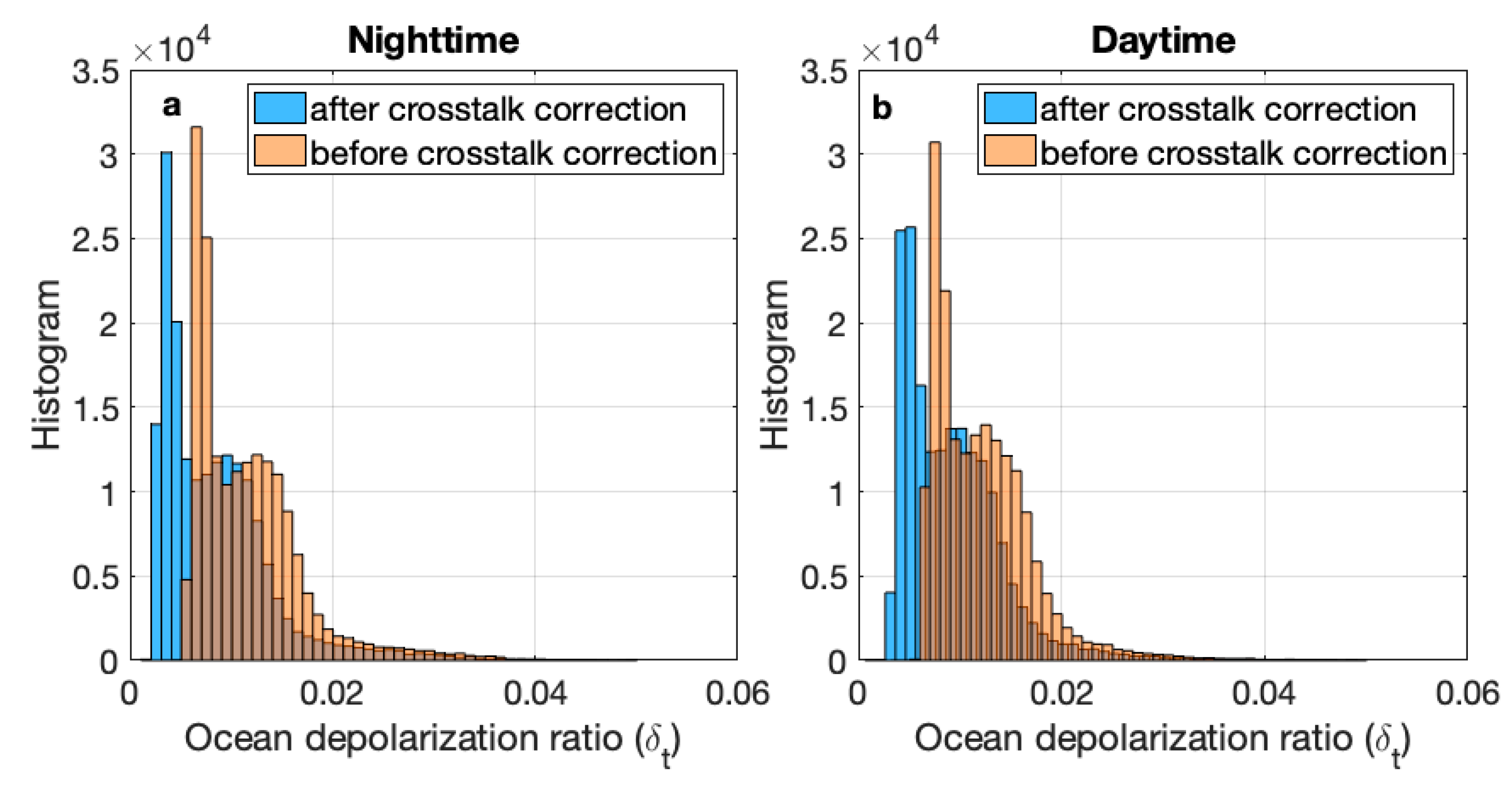
2.3. Effects of Crosstalk on Measured Ocean Backscattered Signals

Even though the crosstalk values are less than 1% over the entire CALIOP mission (Figure 1 and Figure 2), its effects on perpendicular channel ocean signals can still be large [19]. We illustrate this with a heuristic example that assumes the true ocean backscattered signals are β s , t r u e = 1 km−1 sr−1 and β p , t r u e = 100 km−1 sr−1, yielding a total depolarization ratio ( δ t , t r u e = β s , t r u e / β p , t r u e ) of 1% (e.g., as in Figure 3, Figure 4, Figure 5 and Figure 6). Given a polarization crosstalk of 0.5% (e.g., Figure 2), the measured ocean signals given by Equations (1) and (2) will be β s , m e a s u r e d = 1.5 km−1 sr−1 and β p , m e a s u r e d = 99.5 km−1 sr−1, with a corresponding measured depolarization ratio ( δ t . m e a s u r e d = β s , m e a s u r e d / β p , m e a s u r e d ) slightly above 1.5%. The relative error ( Measured value True value True value × 100 % ) of the measured attenuated backscatter coefficient from perpendicular channel ( β s , m e a s u r e d , km−1 sr−1) and total depolarization ratio ( δ t , m e a s u r e d ) due to the crosstalk are ~50%. The particulate backscattering coefficient (bbp, m−1) at 532 nm can be estimated as [5,10]:
b b p β w + β ˜ ( π ) t 2 β s δ t o t a l β ˜ ( π ) t 2 ( 1 10 δ total )
where β ˜ ( π ) (sr−1) is the particulate phase function in the backward direction [31], and t is the ocean surface transmittance (~0.98 at 532 nm) [8]. β w + ( β s δ t o t a l ( 1 10 δ total ) , sr−1) is the column-integrated cross-polarized ocean lidar backscatter, where β s (sr−1) is the ocean surface backscatter estimated from wind speed [13,28] and δ t o t a l is obtained by Equation (13). Equation (8) indicates that the errors associated with total depolarization ratio ( δ t o t a l ) affect the accuracy of CALIOP b b p estimates. From Equation (8), a 50% depolarization ratio error can cause ~59% b b p relative error. The ocean carbon stocks, such as phytoplankton carbon biomass (Cphyto, mg/m3) and total particulate organic carbon (POC, mg/m3) can be directly derived from b b p   [32,33,34]. The uncertainties of Cphyto and POC due to the contribution of b b p uncertainties can be estimated as Δ 2 C p h y t o C p h y t o 2 = Δ 2 b b p b b p 2 and Δ 2 P O C P O C 2 = 0.86 Δ 2 b b p b b p 2 . As a result, a 0.5% polarization crosstalk can cause ~50% errors on measured β s , m e a s u r e d and δ t o t a l , m e a s u r e d , and ~59% relative errors of b b p , which yield the errors of CALIOP retrieved Cphyto and POC of ~59% and ~55%, respectively. Polarization crosstalk is not the only source of uncertainty that can affect the accuracy of CALIOP b b p estimates. Other sources of uncertainty on CALIOP b b p estimates include errors associated with assumptions regarding particulate scattering optical properties, such as particulate depolarization ratios ( δ p ), laser light attenuation in water, particulate phase function in the backward direction, and ocean surface backscatter estimated from wind speed [5]. The uncertainty in the CALIOP b b p due to these error sources is ~37% [5].
The impact of crosstalk increases as the true depolarization ratio decreases and exerts its largest effects in oceanic regions where concentrations of phytoplankton are especially low and hence the true ocean depolarization ratio approaches its minimum. As seen in Figure 5 and Figure 6, the depolarization ratios seen over extensive swaths of the ocean are significantly less than 1%, leading to large crosstalk-induced errors and highlighting the motivation for correcting the data before using the L1 backscatter signals for ocean subsurface retrievals.
From Equations (1) and (2), the crosstalk-corrected attenuated backscatter coefficients ( β p , c o r r e c t , β s , c o r r e c t ) can be derived from the measured signals as:
β p , c o r r e c t ( z ) = β p ,   m e a s u r e d ( z ) / ( 1 C T p 2 s ) , and
β s , c o r r e c t ( z ) = β s , m e a s u r e d ( z ) C T p 2 s × β p , c o r r e c t ( z ) .
The results in Figure 1 indicate that the crosstalk (CTp2s) over CALIOP lifetime can be correctly calculated by two independent methods over two chosen regions (e.g., 0°–40° N and 0°–40° S). The relative differences of the retrieved crosstalk by the two methods and between the two chosen regions are less than 10%. Therefore, the crosstalk-corrected attenuated backscatter coefficients can be derived from the measured signals in a straightforward manner, as indicated in Equations (9) and (10). The correction method is suitable for the global ocean including regions with low-nutrient and low-biomass waters (e.g., Figure 5 and Figure 6). Because our two methods for estimating crosstalk are completely independent and differences between the two (e.g., Figure 1) in terms computing ocean properties (e.g., bbp) are very small (<5%), we have high confidence in our approach. Using CALIOP crosstalk-corrected signals (Equations (9) and (10)) is highly recommended for all ocean subsurface studies.

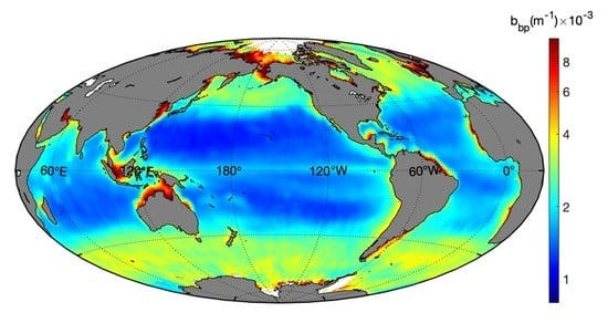
3. Global Ocean Results

This section compares the global ocean depolarization ratios after crosstalk correction with those before crosstalk correction. The integrated cross- ( γ s , sr−1) and co-polarization ( γ p , sr−1) components of the total ocean subsurface backscatters are obtained from CALIOP crosstalk-corrected ocean attenuated backscatter coefficients β p , c o r r e c t ( z ) and β s , c o r r e c t ( z ) as:
γ s = z ( p i 1 ) z ( p i + 3 ) β s , c o r r e c t ( z ) d z ,
γ p = z ( p i 1 ) z ( p i + 3 ) β p , c o r r e c t ( z ) d z .
where pi indicates the altitude index of the peak ocean surface return bin. The total depolarization ratio of ocean water, which includes contributions from water molecules and in-water particulate matter, is defined as:
δ t o t a l = γ s γ p
The seasonal distributions in CALIOP’s total ocean depolarization ratio before crosstalk correction (ratio between Equations (5) and (6)) during both nighttime and daytime are shown in Figure 3 and Figure 4, respectively. Data are seasonally averaged climatologies for the 2008–2020 period and binned to 1° latitude × 1° longitude pixels. For comparison, the seasonal distributions of crosstalk corrected total depolarization ratios using Equation (13) are given in Figure 5 and Figure 6 for nighttime and daytime, respectively.
The ocean depolarization ratios before crosstalk correction shown in Figure 3 and Figure 4 are substantially larger than the depolarization ratios after crosstalk correction (Figure 5 and Figure 6). From Figure 3 and Figure 4, the depolarization ratio is ~1% over most of the permanently stratified oceans—i.e., the low-nutrient and low-biomass waters, between roughly 40° N and 40° S, excluding coastal regions and the Eastern Pacific upwelling regions. However, the crosstalk corrected depolarization ratio (Figure 5 and Figure 6) is ~0.4% over most of these same regions.
Figure 7 presents the histograms of depolarization ratios before (orange) and after (sky blue) crosstalk correction. These results indicate that the mean relative differences in the depolarization ratios before and after crosstalk correction ( δ t o t a l , b e f o r e δ t o t a l , a f t e r δ t o t a l , a f t e r × 100 % ) are ~55% during nighttime and ~42% during daytime. Figure 8 gives the global distributions of (a) particulate backscattering coefficient bbp (m−1) by Equation (8) after the crosstalk correction, (b) the absolute differences of bbp (bbp, beforebbp, after), and (c) the relative differences between the bbp before and after crosstalk correction ( b b p , b e f o r e b b p , a f t e r b b p , a f t e r × 100 % ). Figure 8c indicates that over the low-nutrient, low-biomass waters between roughly 40° N and 40° S, the crosstalk-induced errors in the particulate backscattering coefficient bbp before crosstalk correction are very high and can be as large as 100%. As a result, using CALIOP crosstalk-corrected signals is highly recommended for all ocean subsurface studies.

4. Discussion and Conclusions

In this study, we introduce two approaches to estimate the polarization crosstalk between CALIOP’s 532 nm parallel and perpendicular channels. Both estimates are obtained directly from the CALIOP Level 1 data. Crosstalk magnitudes can be estimated from the clear air depolarization ratios measured between 20 and 30 km (methods 1) and from the ocean backscattered signals in the parallel and perpendicular channels (method 2). The advantage of the second method is that it does not require use of the measured clean air depolarization ratio (which can be contaminated by intermittent injections of stratospheric aerosols), nor does it require explicit knowledge of either the polarization gain ratio or the theoretical value of the clear air depolarization ratio. The CALIOP crosstalk values retrieved by both methods are less than 1% over the CALIPSO entire mission, thus verifying that the engineering design goal of less than 1% crosstalk between the two polarization channels at 532 nm has been successfully accomplished and setting the standard for future space-based lidar missions.
The proposed crosstalk correction methods have been used to correct CALIOP’s measurements of attenuated backscatter coefficients at the near surface of the Earth’s oceans. The global ocean total depolarization ratios are retrieved from the corrected ocean attenuated backscatter coefficients and are compared with those before crosstalk correction. The results indicate the relative errors of ocean total depolarization ratio before crosstalk correction are ~55% during nighttime and ~42% during daytime and can be more than 100% over low-nutrient and low-biomass oceans. Previous analyses of CALIOP data over the regions between roughly 40°N and 40°S would expect to have high relative errors (e.g., Figure 8c) if the optical crosstalk effect between the 532 nm parallel and perpendicular channels was not considered. As a result, using CALIOP crosstalk-corrected signals (Equations (9) and (10)) is highly recommended for all ocean subsurface studies, e.g., calculations of bbp, POC, phytoplankton biomass, etc. Because our two methods for estimating polarization crosstalk are completely independent and differences between the two (e.g., Figure 1) in terms computing ocean properties (e.g., bbp) are very small (<5%), we have high confidence in our approach.
The global distributions of depolarization ratio results (Figure 5 and Figure 6) and particulate backscattering coefficients (Figure 8a) after crosstalk correction clearly exhibit the different phytoplankton communities over the global ocean. For example, the low values of depolarization ratio roughly between 40°N and 40°S latitudes (except in coastal regions) are stable over the annual cycle, indicating low-nutrient, low-biomass waters. The elevated values of depolarization ratio in the Sub-Arctic Oceans and Southern Oceans reflect the large seasonal distributions of phytoplankton blooms with non-spherical particles. Our results strongly support the continued use of CALIOP measurements to study the global plankton system of the upper ocean.

Author Contributions

Conceptualization, X.L. and Y.H.; methodology, Y.H. and X.L.; formal analysis, X.L. and Y.H.; investigation, X.L., Y.H., M.V., S.R. and B.G.; resources, C.T., D.W., M.V., A.O., B.G.; writing—original draft preparation, X.L.; writing—review and editing, all authors; supervision, A.O., R.B., P.L.; project administration, C.T. and P.L.; funding acquisition, X.L. All authors have read and agreed to the published version of the manuscript.

Funding

This research was funded by NASA awards, grant numbers 80NSSC20K0129 and 80NSSC21K0910.

Institutional Review Board Statement

“Not applicable” for studies not involving human or animals.

Informed Consent Statement

“Not applicable” for studies not involving human.

Data Availability Statement

The authors would like to thank the NASA CALIPSO data acquisition and analysis teams for providing the data used in this study. The CALIPSO V4.10 lidar level 1 data used in this study is publicly available and can be freely accessed via https://doi.org/10.5067/CALIOP/CALIPSO/LID_L1-Standard-V4-10, accessed on 13 July 2021.

Conflicts of Interest

The authors declare no conflict of interest.

References

  1. Hunt, W.H.; Winker, D.M.; Vaughan, M.A.; Powell, K.A.; Lucker, P.L.; Weimer, C. CALIPSO Lidar Description and Performance Assessment. J. Atmos. Ocean. Technol. 2009, 26, 1214–1228. [Google Scholar] [CrossRef]
  2. Winker, D.M.; Vaughan, M.A.; Omar, A.; Hu, Y.; Powell, K.A.; Liu, Z.; Hunt, W.H.; Young, S.A. Overview of the CALIPSO Mission and CALIOP Data Processing Algorithms. J. Atmos. Ocean. Technol. 2009, 26, 2310–2323. [Google Scholar] [CrossRef]
  3. Winker, D.M.; Pelon, J.; Coakley, J.A.; Ackerman, S.A.; Charlson, R.J.; Colarco, P.R.; Flamant, P.; Fu, Q.; Hoff, R.M.; Kittaka, C.; et al. The CALIPSO Mission: A Global 3D View of Aerosols and Clouds. Bull. Am. Meteorol. Soc. 2010, 91, 1211–1229. [Google Scholar] [CrossRef]
  4. Powell, K.A.; Hostetler, C.A.; Vaughan, M.A.; Lee, K.-P.; Trepte, C.R.; Rogers, R.R.; Winker, D.M.; Liu, Z.; Kuehn, R.E.; Hunt, W.H.; et al. CALIPSO Lidar Calibration Algorithms. Part I: Nighttime 532-Nm Parallel Channel and 532-Nm Perpendicular Channel. J. Atmos. Ocean. Technol. 2009, 26, 2015–2033. [Google Scholar] [CrossRef]
  5. Behrenfeld, M.J.; Hu, Y.; Hostetler, C.A.; Dall’Olmo, G.; Rodier, S.D.; Hair, J.W.; Trepte, C.R. Space-Based Lidar Measurements of Global Ocean Carbon Stocks. Geophys. Res. Lett. 2013, 40, 4355–4360. [Google Scholar] [CrossRef]
  6. Lu, X.; Hu, Y. Estimation of Particulate Organic Carbon in the Ocean from Space-Based Polarization Lidar Measurements. In Proceedings of the SPIE Asia-Pacific Remote Sensing, Beijing, China, 10 December 2014; Volume 9261, pp. 92610Z-1–92610Z-8. [Google Scholar]
  7. Lacour, L.; Larouche, R.; Babin, M. In Situ Evaluation of Spaceborne CALIOP Lidar Measurements of the Upper-Ocean Particle Backscattering Coefficient. Opt. Express 2020, 28, 26989–26999. [Google Scholar] [CrossRef] [PubMed]
  8. Lu, X.; Hu, Y.; Pelon, J.; Trepte, C.; Liu, K.; Rodier, S.; Zeng, S.; Lucker, P.; Verhappen, R.; Wilson, J.; et al. Retrieval of Ocean Subsurface Particulate Backscattering Coefficient from Space-Borne CALIOP Lidar Measurements. Opt. Express 2016, 24, 29001–29008. [Google Scholar] [CrossRef]
  9. Behrenfeld, M.J.; Gaube, P.; Della Penna, A.; O’Malley, R.T.; Burt, W.J.; Hu, Y.; Bontempi, P.S.; Steinberg, D.K.; Boss, E.S.; Siegel, D.A.; et al. Global Satellite-Observed Daily Vertical Migrations of Ocean Animals. Nature 2019, 576, 257–261. [Google Scholar] [CrossRef] [PubMed]
  10. Bisson, K.M.; Boss, E.; Werdell, P.J.; Ibrahim, A.; Behrenfeld, M.J. Particulate Backscattering in the Global Ocean: A Comparison of Independent Assessments. Geophys. Res. Lett. 2021, 48, e2020GL090909. [Google Scholar] [CrossRef]
  11. Behrenfeld, M.J.; Hu, Y.; O’Malley, R.T.; Boss, E.S.; Hostetler, C.A.; Siegel, D.A.; Sarmiento, J.L.; Schulien, J.; Hair, J.W.; Lu, X.; et al. Annual Boom-Bust Cycles of Polar Phytoplankton Biomass Revealed by Space-Based Lidar. Nat. Geosci. 2017, 10, 118–122. [Google Scholar] [CrossRef]
  12. Dionisi, D.; Brando, V.E.; Volpe, G.; Colella, S.; Santoleri, R. Seasonal Distributions of Ocean Particulate Optical Properties from Spaceborne Lidar Measurements in Mediterranean and Black Sea. Remote Sens. Environ. 2020, 247, 111889. [Google Scholar] [CrossRef]
  13. Lu, X.; Hu, Y.; Trepte, C.; Zeng, S.; Churnside, J.H. Ocean Subsurface Studies with the CALIPSO Spaceborne Lidar. J. Geophys. Res. Ocean. 2014, 119, 4305–4317. [Google Scholar] [CrossRef]
  14. Churnside, J.; McCarty, B.; Lu, X. Subsurface Ocean Signals from an Orbiting Polarization Lidar. Remote Sens. 2013, 5, 3457–3475. [Google Scholar] [CrossRef] [Green Version]
  15. Hostetler, C.A.; Behrenfeld, M.J.; Hu, Y.; Hair, J.W.; Schulien, J.A. Spaceborne Lidar in the Study of Marine Systems. Annu. Rev. Mar. Sci. 2018, 10, 121–147. [Google Scholar] [CrossRef] [Green Version]
  16. Jamet, C.; Ibrahim, A.; Ahmad, Z.; Angelini, F.; Babin, M.; Behrenfeld, M.J.; Boss, E.; Cairns, B.; Churnside, J.; Chowdhary, J.; et al. Going Beyond Standard Ocean Color Observations: Lidar and Polarimetry. Front. Mar. Sci. 2019, 6, 251. [Google Scholar] [CrossRef]
  17. Churnside, J.H.; Shaw, J.A. Lidar Remote Sensing of the Aquatic Environment: Invited. Appl. Opt. 2020, 59, C92–C99. [Google Scholar] [CrossRef]
  18. Chris, A.H.; Liu, Z.; Reagan, J.; Vaughan, M.; Winker, D.; Osborn, M.; Hunt, W.; Powell, K.; Trepte, C. CALIOP Algorithm Theoretical Basis Document Calibration and Level 1 Data Products. Pc-Sci-201 Release 1.0, 2006. Available online: https://www-calipso.larc.nasa.gov/resources/pdfs/PC-SCI-201v1.0.pdf (accessed on 13 July 2021).
  19. Lu, X.; Hu, Y.; Yang, Y.; Neumann, T.A.; Omar, A.; Baize, R.; Vaughan, M.; Rodier, S.; Getzewich, B.; Trepte, C.; et al. New Ocean Subsurface Optical Properties from Space Lidars: CALIOP/CALIPSO and ATLAS/ICESat-2. Earth Space Sci. 2021. [Google Scholar] [CrossRef]
  20. Pitts, M.C.; Poole, L.R.; Gonzalez, R. Polar Stratospheric Cloud Climatology Based on CALIPSO Spaceborne Lidar Measurements from 2006 to 2017. Atmos. Chem. Phys. 2018, 18, 10881–10913. [Google Scholar] [CrossRef] [Green Version]
  21. Vaughan, M.; Pitts, M.; Trepte, C.; Winker, D.; Detweiler, P.; Garnier, A.; Getzewich, B.; Hunt, W.; Lambeth, J.; Lee, K.-P.; et al. Cloud—Aerosol LIDAR Infrared Pathfinder Satellite Observations (CALIPSO) Data Management System Data Products Catalog. Document No: PC-SCI-503, 2020. Available online: https://www-calipso.larc.nasa.gov/products/CALIPSO_DPC_Rev4x92.pdf (accessed on 13 July 2021).
  22. Kar, J.; Vaughan, M.A.; Lee, K.-P.; Tackett, J.L.; Avery, M.A.; Garnier, A.; Getzewich, B.J.; Hunt, W.H.; Josset, D.; Liu, Z.; et al. CALIPSO Lidar Calibration at 532 Nm: Version 4 Nighttime Algorithm. Atmos. Meas. Tech. 2018, 11, 1459–1479. [Google Scholar] [CrossRef] [PubMed] [Green Version]
  23. Getzewich, B.J.; Vaughan, M.A.; Hunt, W.H.; Avery, M.A.; Powell, K.A.; Tackett, J.L.; Winker, D.M.; Kar, J.; Lee, K.-P.; Toth, T.D. CALIPSO Lidar Calibration at 532 Nm: Version 4 Daytime Algorithm. Atmos. Meas. Tech. 2018, 11, 6309–6326. [Google Scholar] [CrossRef] [Green Version]
  24. Siddaway, J.M.; Petelina, S.V. Transport and Evolution of the 2009 Australian Black Saturday Bushfire Smoke in the Lower Stratosphere Observed by OSIRIS on Odin. J. Geophys. Res. Atmos. 2011, 116, 1–9. [Google Scholar] [CrossRef] [Green Version]
  25. Khaykin, S.; Legras, B.; Bucci, S.; Sellitto, P.; Isaksen, L.; Tencé, F.; Bekki, S.; Bourassa, A.; Rieger, L.; Zawada, D.; et al. The 2019/20 Australian Wildfires Generated a Persistent Smoke-Charged Vortex Rising up to 35 km Altitude. Commun. Earth Environ. 2020, 1, 22. [Google Scholar] [CrossRef]
  26. Peterson, D.A.; Campbell, J.R.; Hyer, E.J.; Fromm, M.D.; Kablick, G.P.; Cossuth, J.H.; DeLand, M.T. Wildfire-Driven Thunderstorms Cause a Volcano-like Stratospheric Injection of Smoke. NPJ Clim. Atmos. Sci. 2018, 1, 30. [Google Scholar] [CrossRef] [Green Version]
  27. Christian, K.; Yorks, J.; Das, S. Differences in the Evolution of Pyrocumulonimbus and Volcanic Stratospheric Plumes as Observed by CATS and CALIOP Space-Based Lidars. Atmosphere 2020, 11, 1035. [Google Scholar] [CrossRef]
  28. Hu, Y.; Stamnes, K.; Vaughan, M.; Pelon, J.; Weimer, C.; Wu, D.; Cisewski, M.; Sun, W.; Yang, P.; Lin, B.; et al. Sea Surface Wind Speed Estimation from Space-Based Lidar Measurements. Atmos. Chem. Phys. 2008, 8, 3593–3601. [Google Scholar] [CrossRef] [Green Version]
  29. Lu, X.; Hu, Y.; Liu, Z.; Zeng, S.; Trepte, C. CALIOP Receiver Transient Response Study. In Proceedings of the SPIE 8873, Polarization Science and Remote Sensing VI, San Diego, CA, USA, 27 September 2013; Volume 8873, pp. 887316-1–887316-9. [Google Scholar] [CrossRef]
  30. Lu, X.; Hu, Y.; Trepte, C.; Liu, Z. A Super-Resolution Laser Altimetry Concept. IEEE Geosci. Remote Sens. Lett. 2014, 11, 298–302. [Google Scholar] [CrossRef]
  31. Sullivan, J.M.; Twardowski, M.S. Angular Shape of the Oceanic Particulate Volume Scattering Function in the Backward Direction. Appl. Opt. 2009, 48, 6811–6819. [Google Scholar] [CrossRef]
  32. Stramski, D.; Reynolds, R.A.; Kahru, M.; Mitchell, B.G. Estimation of Particulate Organic Carbon in the Ocean from Satellite Remote Sensing. Science 1999, 285, 239–242. [Google Scholar] [CrossRef] [PubMed]
  33. Behrenfeld, M.J.; Boss, E.; Siegel, D.A.; Shea, D.M. Carbon-Based Ocean Productivity and Phytoplankton Physiology from Space. Glob. Biogeochem. Cycles 2005, 19, 1–14. [Google Scholar] [CrossRef]
  34. Lu, X.; Hu, Y.; Yang, Y.; Bontempi, P.; Omar, A.; Baize, R. Antarctic Spring Ice-Edge Blooms Observed from Space by ICESat-2. Remote Sens. Environ. 2020, 245, 111827. [Google Scholar] [CrossRef]
Figure 1. Time series of crosstalk calculated from CALIOP L1 data by methods 1 and 2 from June 2006. to November 2020 over two chosen regions 0°–40° N (green by method 1 and blue by method 2) and 0°–40° S (black by method 1 and pink by method 2). The dashed blue line indicates when CALIOP was switched from the primary laser to the backup laser (i.e., February 2009). The discrete jumps in April 2009, September/October 2017, and February 2020 by method 1 are most likely due to the depolarizing smoke injected into the stratosphere. See details in text.
Remotesensing 13 02769 g001
Figure 2. Time series of crosstalk difference between night and day ( C T p 2 s , n i g h t C T p 2 s , d a y ) calculated from CALIOP L1 ocean signals by method 2 from June 2006 to November 2020 over two chosen regions 0°–40° N (red) and 0°–40° S (dark blue). The dashed blue line indicates when CALIOP was switched from the primary laser to the backup laser (i.e., February 2009).
Remotesensing 13 02769 g002
Figure 3. Seasonal distributions of CALIOP total depolarization ratio ( δ t o t a l , %) at nighttime before crosstalk correction. (a) March–May; (b) June–August; (c) September–November; (d) December–February. Data are seasonal average climatology for the 2006–2020 period and have been averaged to 1° latitude × 1° longitude pixels.
Remotesensing 13 02769 g003
Figure 4. Same with Figure 3 but for daytime results before crosstalk correction.
Remotesensing 13 02769 g004
Figure 5. Seasonal distributions of CALIOP total depolarization ratio ( δ t o t a l , %) at nighttime after crosstalk correction. (a) March–May; (b) June–August; (c) September–November; (d) December–February. Data are seasonal average climatology for the 2008–2020 period and have been averaged to 1° latitude × 1° longitude pixels.
Remotesensing 13 02769 g005
Figure 6. Same with Figure 5 but for daytime results after crosstalk correction.
Remotesensing 13 02769 g006
Figure 7. Ocean total depolarization ratio comparisons after (sky blue color) and before (orange color) crosstalk corrections during (a) nighttime and (b) daytime.
Remotesensing 13 02769 g007
Figure 8. (a) Global distribution of the particulate backscattering coefficient bbp (m−1) after the crosstalk correction. (b) Absolute differences of bbp (m−1) before and after the crosstalk correction ( b b p , b e f o r e b b p , a f t e r ). (c) Relative differences of bbp before and after crosstalk correction ( b b p , b e f o r e b b p , a f t e r b b p , a f t e r × 100 % ). Data are climatological annual averages for the 2008–2020 period and have been averaged to 1° latitude × 1° longitude pixels.
Remotesensing 13 02769 g008
Publisher’s Note: MDPI stays neutral with regard to jurisdictional claims in published maps and institutional affiliations.

