Article

Soil Moisture Estimates in a Grass Field Using Sentinel-1 Radar Data and an Assimilation Approach

Dipartimento di Ingegneria Civile, Ambientale e Architettura, Università di Cagliari, 09123 Cagliari, Italy
*
Author to whom correspondence should be addressed.
Remote Sens. 2021, 13(16), 3293; https://doi.org/10.3390/rs13163293
Submission received: 18 June 2021 / Revised: 6 August 2021 / Accepted: 12 August 2021 / Published: 20 August 2021
(This article belongs to the Section Biogeosciences Remote Sensing)

Abstract

:
The new constellation of synthetic aperture radar (SAR) satellite, Sentinel-1, provides images at a high spatial resolution (up to 10 m) typical of radar sensors, but also at high time resolutions (6–12 revisit days), representing a major advance for the development of operational soil moisture mapping at a plot scale. Our objective was to develop and test an operational approach to assimilate Sentinel 1 observations in a land surface model, and to demonstrate the potential of the use of the new satellite sensors in soil moisture predictions in a grass field. However, for soil moisture retrievals from Sentinel 1 observations in grasslands, there is still the need to identify robust and parsimonious solutions, accounting for the effects of vegetation attenuation and their seasonal variability. In a grass experimental site in Sardinia, where field measurements of soil moisture were available for the 2016–2018 period, three common retrieval methods have been compared to estimate soil moisture from Sentinel 1 data, with increasing complexity and physical interpretation of the processes: the empirical change detection method, the semi-empirical Dubois model, and the physically-based Fung model. In operational approaches for soil moisture mapping from remote sensing, the parameterization simplification of soil moisture retrieval techniques is encouraged, looking for parameter estimates without a priori information. We have proposed a simplified approach for estimating a key parameter of retrieval methods, the surface roughness, from the normalized difference vegetation index (NDVI) derived by simultaneous Sentinel 2 optical observations. Soil moisture was estimated better using the proposed approach and the Dubois model than by using the other methods, which accounted vegetation effects through the common water cloud model. Furthermore, we successfully merged radar-based soil moisture observations and a land surface model, through a data assimilation approach based on the Ensemble Kalman filter, providing robust predictions of soil moisture.

Graphical Abstract

1. Introduction

The state of soil moisture is a key variable of land surface processes controlling surface water and energy balances [1,2,3,4]. Nowadays, remote sensors provide an unprecedented opportunity to monitor soil moisture at a high time frequency over large spatial scales [5,6,7,8]. A variety of infrared and microwave (both active and passive) sensors operating from laboratory, aircraft, and satellite platforms have been tested for soil moisture retrieval, and the potentials and limitations of each of these remote sensing techniques have been well documented [7,9,10,11]. The main advantage of the radar, an active sensor, is that it provides observations at much higher spatial resolutions (tens of meters) than those (tens of kilometers) of passive satellite sensors (e.g., radiometers or scatterometers) [12,13,14]. The high spatial resolution of radar is a key qualification for soil moisture mapping of small hydrologic basins, such as Mediterranean basins that are typically characterized by a rugged topography and a high spatial variability of physiographic properties [15,16] Furthermore, in Mediterranean basins under water-limited conditions, soil moisture ranges frequently moving to extreme opposite moisture conditions (from dry to wet or vice-versa) over a short time (e.g., daily, weekly) [17,18,19], highlighting the need for soil moisture mapping at a high frequency.
In this sense, the new constellation of synthetic aperture radar (SAR) satellites, Sentinel-1 A (from April 2014) and Sentinel-1B (from April 2016), provides images at high spatial resolution (up to 10 m) typical of radar sensors, but also at high time resolutions (6–12 revisit days), representing a major advance for the development of operational soil moisture mapping at plot scale [20,21,22].
Several methods have been developed to estimate soil moisture over bare soil surfaces from SAR observations, varying from physical models (e.g., the Integral Equation Model (IEM; Fung et al. [23]), the Advanced Integral Equation Model (AIEM; [24]), and the Integral Equation Model for Multiple Scattering [25], to empirical and semi-empirical models [24,26,27,28]. Recent efforts have estimated soil moisture in bare soil plots from Sentinel 1 data using both physical models [29,30,31,32] and empirical approaches [33,34,35,36]. The unprecedented high frequency of the Sentinel 1 satellite passes has also encouraged the use of simple change detection techniques [5,37], where soil moisture is estimated linearly scaling observed radar backscatter.
Grass species are common on all continents except Antarctica, and grasslands cover approximately 26% of terrestrial areas globally [38,39]. To estimate soil moisture from SAR images in grasslands, the main difficulties are that soil moisture, surface roughness, and vegetation cover all have an important and nearly equal effect on radar backscatter [31,40,41,42,43,44,45], and grass cover is not constant over time but changes seasonally [46,47]. Empirical relationships have been proposed to account for vegetation effects on a backscatter SAR signal [43]), relating the SAR signal with vegetation indexes, such as the normalized difference vegetation index (NDVI), which can be estimated from concomitant optical data. However, the most common approach is based on the water cloud model (WCM) [44,48,49,50], where the vegetation contribution is computed from vegetation parameters (e.g., the NDVI), and vegetation effects are subtracted to radar backscatter, which is then related to bare soil water contents.
Most previous efforts [43,45,51] have investigated the effects of vegetation on SAR signals using an instantaneous satellite image and relating the SAR signal to the spatial variability of vegetation, somehow accounting also for the effects of the spatial variability of other physiographic properties on soil moisture [3,52]. Nowadays the optical Sentinel 2 data [6] provide observations of vegetation indices at high spatial (10 m) and temporal (5 days) resolutions, similar to Sentinel 1 observations. Numerous efforts have combined Sentinel 1 and Sentinel 2 data for soil moisture estimation using the WCM [35,50,51], the change detection method [5,53], a neural network technique [29], and a machine learning regression algorithm [54]. The use of almost simultaneous observations of Sentinel 1 and Sentinel 2 provides an opportunity to investigate the effects of vegetation on SAR signals for individual locations at a plot-scale over long time periods without the effects of the variability of other physiographic properties.
The parameterization simplification of soil moisture retrieval techniques is encouraged in operational approaches for soil moisture mapping from remote sensors, looking for parameter estimates without a priori information [55]. Radar surface roughness is one of the key parameters of most common models (e.g., Fung et al. [23] and Dubois et al. [27] models. Surface roughness is typically assumed to be constant over a relatively short time period [44,56], but when long periods are considered, this assumption can hardly be preserved. Interestingly, Capodici et al. [52] estimated a linear increase of surface roughness with NDVI for a maize field relative to a short growing season (April–August 2006). With the objective of simplifying parameterization, we looked for a surface roughness (NDVI relationship effective over all seasons) to be used with common retrieval models such as the Fung et al. [23] and Dubois et al. [27] models, which were able to account for grass cover effects on radar signals. For comparison, the common WCM is also used to account for vegetation contributions.
Data assimilation techniques are being developed to guide land surface models (LSM) with periodic observations of certain state variables, such as surface soil moisture, observed indirectly by remote sensing platforms [57,58,59,60,61,62,63,64,65,66]. Montaldo and Albertson [67] and Montaldo et al. [68] developed a procedure for soil moisture assimilation at the plot scale using the Ensemble Kalman filter (EnKF; Refs. [66,69,70] in a force-restore based land surface model (LSM). However, Montaldo et al. [68] used observations from frequency domain reflectometer (FDR) probes installed in the field as a proxy for remote sensing observations of soil moisture due to the absence of radar long data sets at high spatial and temporal resolutions at that time. Nowadays, the unprecedented high temporal frequency of Sentinel 1 observations provides the opportunity to finally achieve operational procedures for soil moisture assimilation at fine spatial scales. The first efforts by Pan et al. [8] and Zhuo et al. [56] assimilated Sentinel 1 -derived soil moisture in the WOFOST model using the EnKF. The soil moisture assimilation system was applied to estimate winter yield and for a short growing season only and used simple approaches for soil moisture retrieval from Sentinel 1 observations (change detection method in Pan et al. [8] and an empirical relationship between radar backscattering and soil moisture in Zhuo et al. [56]). To develop an operational data assimilation approach for soil moisture predictions using the attractive Sentinel 1 observations there is still the need to identify robust and parsimonious solutions for soil moisture retrievals in vegetated fields. Starting from Montaldo et al. [68], we assimilated Sentinel 1-derived soil moisture estimates in the LSM, using an EnKF-based assimilation approach for soil moisture predictions, and accounting for the effects of vegetation on SAR signals.
The experimental grass field of Orroli in Sardinia [47,71,72] provides an interesting case study for testing an operative approach for soil moisture estimation due to its strong interannual and seasonal rain variability [73] affecting soil moisture dynamics. The field site was monitored for a three-year period (2016–2018), during which Sentinel 1 and Sentinel 2 observations and soil moisture measurements were available. In this way, the following objectives were addressed:
-
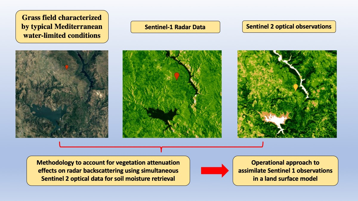
To test the potential of Sentinel 1 for soil moisture estimation in a grass field characterized by typical Mediterranean water-limited conditions;
-
To compare and revise some common retrieval models for soil moisture estimation from Sentinel 1 data, proposing a simplified and robust solution to account for vegetation attenuation effects on radar backscattering using simultaneous Sentinel 2 optical data;
-
To develop and test an operational approach to assimilate Sentinel 1 observations in a land surface model, to demonstrate the potential of the use of the new satellite sensors in soil moisture predictions in a grass field.

2. Materials and Methods

The proposed assimilation approach includes radar-based soil moisture observations, the land surface model, and the EnKF. We compared several methods for soil moisture retrieval from radar data, and, to account for the contribution of vegetation on radar, we evaluated an existing method, the WCM, and proposed a simplified approach, testing them with field data of the Sardinian grass site. In the following sections, the case study and field campaign, the satellite data, methods for soil moisture retrieval from radar information, and the assimilation approach are described.

2.1. Sardinian Case Study

The experimental grass site was in Orroli, Italy (39°41′12.57″ N, 9°16′30.34″ E, 560 m a. s. l.), on the island of Sardinia [47] The climate at the site is maritime Mediterranean, with a mean annual precipitation (1922–2018) of 612 mm and mean historical monthly precipitation ranging from 11 mm in July to 102 mm in December. The mean annual air temperature is 14.6 °C, and the mean historical monthly temperature ranges from a minimum of 7.1 °C in January to a maximum of 23.7 °C in July.
Grasses (Bellium bellidioides, Bellis perennis; Avena fatua, Hordeum murinum) reach their maximum growth (~25 cm) in spring. Grass then dies yellowing at the end of summer (the driest season), as is common for Mediterranean species [46].
The land gently sloped approximately 4.6°; the soil, which was 17 cm in deep (coincident with the root zone depth) above a fractured basalt, was a silt loam with mean bulk density of 1.48 g/cm3 and a porosity of 53% [17]. The grass root density was 0.5–1.0 kg/m3.
Five frequency domain reflectometer probes (FDR, Campbell Scientific Model CS-616) were inserted in the grass field to monitor moisture (θ) in the thin soil layer from May 2003 to August 2018 (with several gaps due to instrument failure). FDR calibration ( θ = 2.456 7.135 τ + 6.701 τ 2 1.884 τ 3 where τ is the output period in milliseconds) was performed using 15 periodic gravimetric water content samples taken over a wide range of θ (0.08–0.52 m3 m−3) near the probes. Micrometeorological observations from 2003 onwards are also available for the Orroli site [17,47].
Soil moisture was also monitored in another grass field (39°41′15.8″ N, 9°13′18.5″ E, 480 m a. s. l.) close to the Orroli site (5 km away), using portable soil moisture probes (ThetaProbe ML3) opportunely tested with gravimetric measurements, and sampling eight points in an area of approximately 60 m × 100 m in size. Soil moisture was monitored during eight days of 2017 (day of the year, DOY, 40, 76, 83, 103, 125, 135, 151,173) and five days of 2018 (DOY 157, 166, 190, 204, 211). The soil was a silt loam with mean bulk density of 1.38 g/cm3, and a porosity of 45%. This secondary case study provided the opportunity to further validate the proposed method for soil moisture estimation from Sentinel 1 data.

2.2. Satellite Data

Two types of remote sensors belonging to the Sentinel satellite constellation were examined and coupled. The first was the SAR mounted on Sentinel 1 to detect the dielectric constant of the surface soil, which is related to soil moisture, and the second was the multispectral optical radiometer mounted on Sentinel 2, to detect vegetation characteristics.
The Sentinel 1 radar data were derived from S1A and S1B satellites, which carry a C-band synthetic-aperture radar instrument, and the level-1 Ground Range Detected GRD was used. The images were calibrated, corrected from the noise with a Lee filter 7 × 7, and resampled at a 30 m spatial resolution. The S1A images were available from January 2016, and we selected the VV polarization, since VV polarization is higher sensitive to soil moisture [45,74] and less sensitive to vegetation compared to VH polarization [75]. From September 2016, the S1B satellite images were also available, so that the double information coming from the two satellites (S1A and S1B) was available every six days approximately, but in two different acquisition modes, descending (at ~05:28 AM) and ascending (at ~05:28 PM) respectively. In total, Sentinel 1 data were collected for 153 days from January 2016 to August 2018, and the corresponding σ0vv backscattering coefficients from S1A and S1b images were acquired.
The images of the Sentinel 2 radiometer were acquired at the L1C level, and afterwards they were atmospherically corrected with Sen2Cor tool of the Sentinel Application platform (SNAP), or directly at the L2A level (already corrected). The optical data were used to estimate the NDVI at high spatial (10 m) and temporal (≈5 days) resolutions. Optical data were resampled at a 30 m spatial resolution as radar images, and the NDVI was available for 74 days from January 2016 to August 2018. Due to the lack of NDVI data from Sentinel 2 during a few months in 2016 and 2017, we also acquired eight operational Land Imager (OLI)—Landsat 8 data at a 30 m spatial resolution to increase the NDVI dataset.
To test the data assimilation approach, Sentinel 1 and Sentinel 2 data from August 2018 to July 2020 were also acquired.

2.3. Methods for Soil Moisture Retrieval from Sentinel 1 Data

To estimate soil moisture from Sentinel 1 data, three common methods have been used, with increasing complexity and physical interpretation of the processes: the empirical change detection method [5], the semi-empirical Dubois et al. [31] method, and the physically-based Fung et al. [23] method. The change detection method estimates soil moisture from σ0vv directly, while the Dubois et al. [27] and Fung et al. [23] methods compute the ε dielectric constant from σ0vv, so that a further step is needed to estimate θ from ε. To relate θ with ε through the Γ operator, we used the common Topp et al. [76] equation [36,41,77]:
θ = Γ ε = 530 + 292 ε 5.5 ε 2 + 0.043 ε 3 10 4

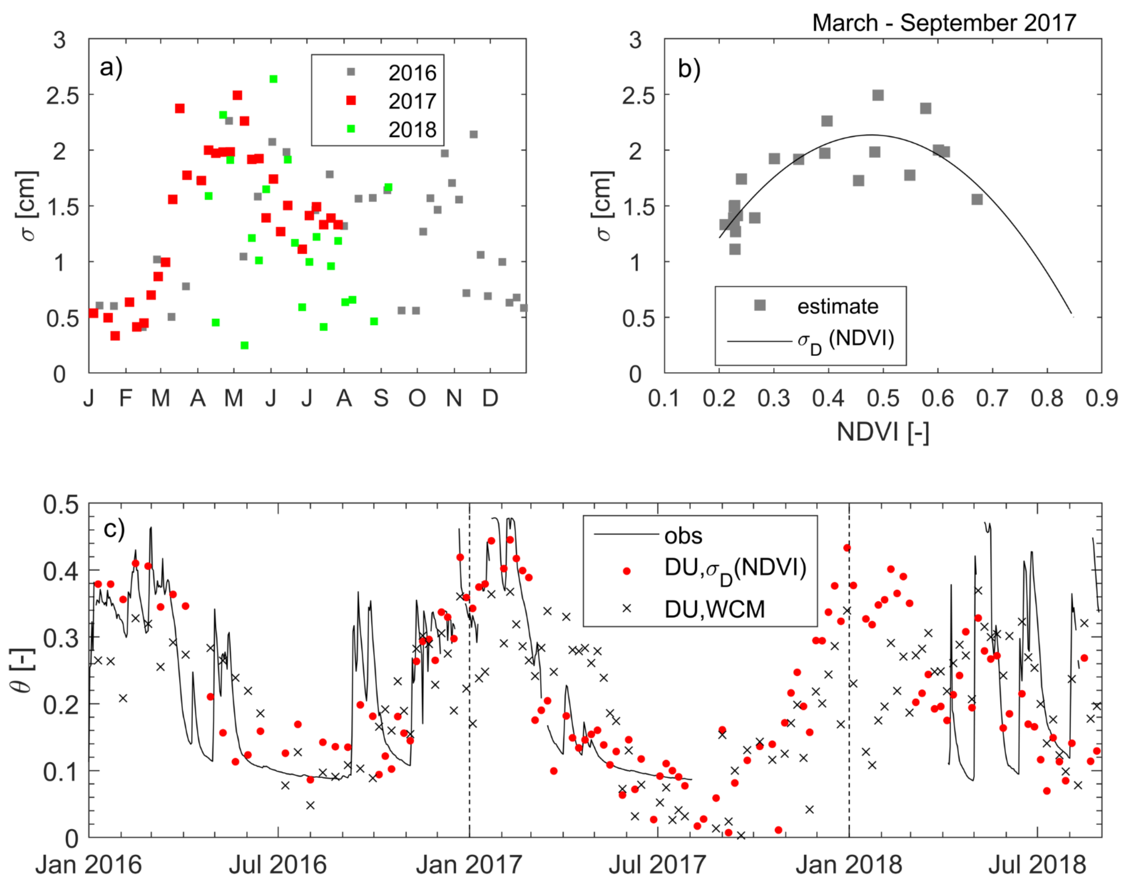
2.3.1. The Revised Change Detection Method

The change detection method estimates θ linearly scaling the observed radar backscatter between the minimum (σ0dry) and maximum (σ0wet) backscatter values observed over the investigated period; these are considered to be equivalent to the dry and wet soil references, respectively [5]. The method’s assumption is that factors influencing the radar backscatter signal vary over time, with vegetation and surface roughness affecting long-term changes in σ0vv, whereas short-term variations of backscattering are associated with moisture variations. The high temporal resolution of Sentinel-1 SAR time series is a precondition for the use of the method. We revised the Urban et al. [5] method:
θ = θ m i n + σ 0 σ d r y 0 σ w e t 0 σ d r y 0 θ s θ m i n
where we rescaled θ between a minimum (θmin) and a maximum (the saturated soil moisture condition, θs) amount of soil moisture, which were characteristics of the soil type, and could be determined from the observed soil moisture; σ0dry and σ0wet were estimated from the lowest and the highest backscatter values observed over the investigated period, respectively [5]. Hereafter, we indicated with “CD” the revised change detection method.

2.3.2. The Semi-Empirical Model of Dubois et al. 1995

The Dubois et al. [27] model accounts for co-polarized backscattering only and relates the backscattering signal with the dielectric constant of the ground. The model is restricted to co-polarization channels (VV or HH). Here, only the VV relation was used:
σ v v 0 = 10 2.35 cos 3 β sin 3 β 10 0.046 ε tan β ( k σ sin β ) 1.1 λ 0.7
where λ is the wavelength, k is the wave number equal to 2π/λ, σ is the surface roughness, and β is the local incident angle related to radar beam angle and the latitude, exposition and slope of the site. The inversion of (3) allowed us to estimate the dielectric constant from σ0vv radar observations, knowing surface roughness and the specific radar configuration parameters (wavelength and incidence angle). While radar configuration parameters were known, σ was undetermined.
Commonly, prescribed or field estimated values of σ can be used as a constant over time to estimate ε with (3). When simultaneous soil moisture field measurements and radar observations are available, (3) can be used in inverse mode for estimating σ. Indeed, we derived a “measured” ε dielectric constant inverting (1) using the θ measurements at the field, then using σ0vv from ε we estimated σ by inverting (3) at each satellite pass. In this way, the variability of σ with grass growth was investigated. We hereafter refer to the Dubois et al. [27] model as “DU”.

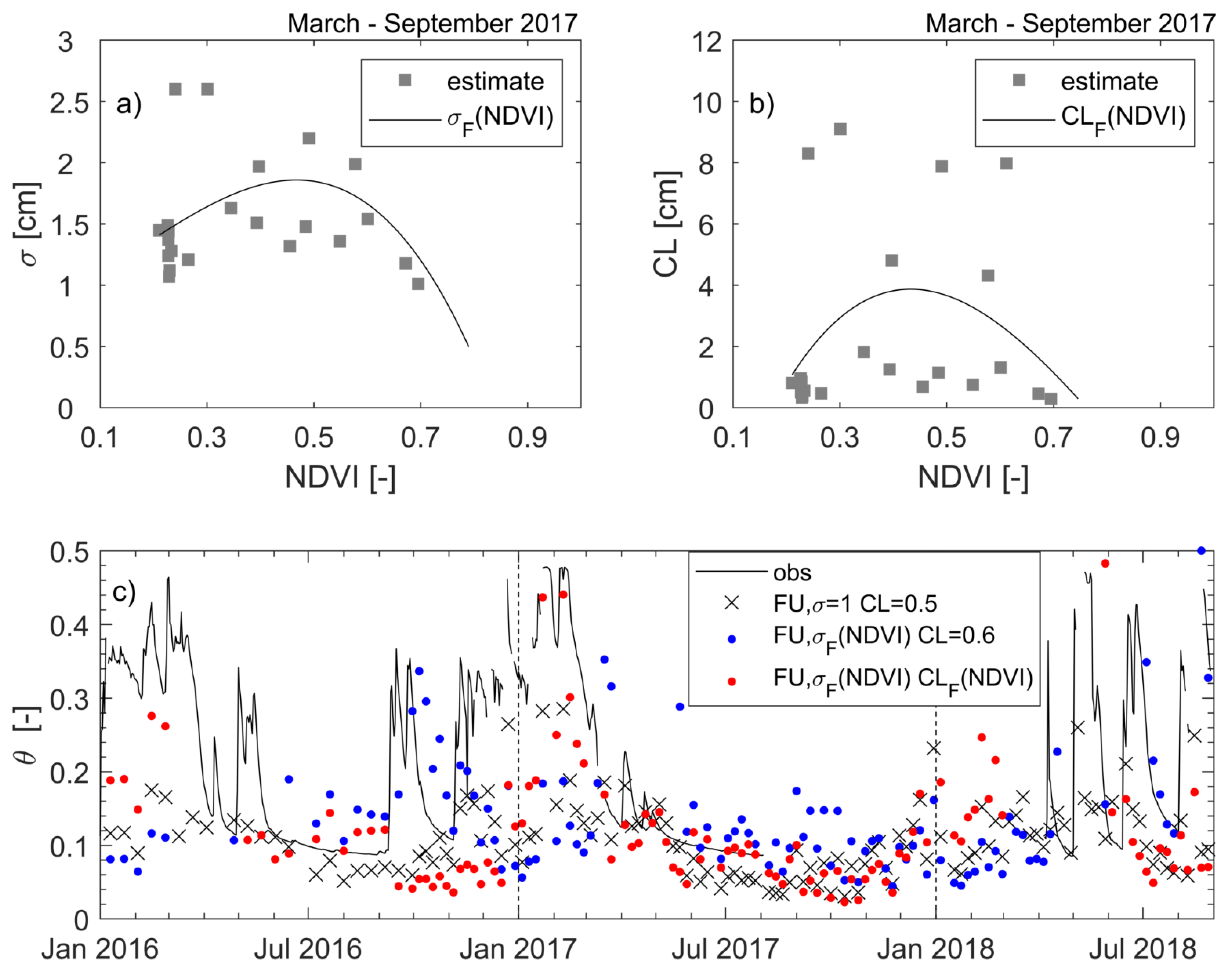
2.3.3. The Physical Model of Fung et al., 1992

The Fung et al. [23] model is a radioactive transfer model that estimates the backscattering coefficient for a random roughness surface, knowing the antenna radar characteristics (the wavelength, the frequency, the polarization and the angle of view) and the properties of the investigated surface (ε, the μ electromagnetic permeability, σ, the CL correlation length, and the inclination of a specific point with respect their vertical-azimuth). Considering smooth to moderately rough natural surfaces (with < 3) the backscattering coefficient was estimated as:
σ v v 0 = k 2 2 exp 2 k z 2 σ 2 n = 1 σ 2 n I v v n W n 2 k x , 0 n !
where kz is equal to k cos β, and kx is equal to k sin β. The term I v v n is given:
I v v n = 2 k z ) n f v v exp ( k z 2 σ 2 + k z n F v v k x , 0 + F v v k x , 0 2
where:
f V V = 2 R v cos β
F v v k x , 0 + F v v k x , 0 = 2 sin β ( 1 + R v ) 2 cos β 1 1 ε + μ ε sin 2 β ε cos 2 β ε 2 cos 2 β
where Rv is the surface reflection coefficient given by the Fresnel reflection equation as a function of the local incident angle and the dielectric constant based on the polarization sensor, and W n 2 k x , 0 is the Fourier transform of the nth power of the surface autocorrelation function, which is related to CL by an exponential distribution.
To estimate ε from σ0vv observations, Equation (4) (together with (5)–(7)) needs to be inverted, and two parameters, σ and CL, need to be defined. Usually, prescribed or field estimated values of σ and CL are used, assuming that they are constant over time. When field soil moisture observations are available, Equation (4) can be used in inverse mode to estimate σ and CL for each satellite pass, using simultaneous radar observations. Indeed, from θ measured in the field, a “measured” ε dielectric constant can be derived inverting (1), and ε can be used in (4), to obtain σ and CL from σ0vv observations. However, since two parameters are unknown, two equations are needed. Sentinel 1 provided two daily passes (S1A and S1B), so that two σ0vv were available daily, and two Equation (4) could be used. Indeed, assuming that the soil moisture measured at the field remained approximately constant throughout the day, the system of two Equation (4) could be solved to estimate the two unknown parameters at each satellite pass. We investigated the time variabilities of σ and CL with grass growth at the field site, relating them to simultaneous NDVI observations.
The Fung et al. [23] model is from here on referred to as “FU”.

2.3.4. Removal of Grass Cover Contribution from Radar Backscattering

To account for the contribution of vegetation and the attenuation on radar backscattering we first used the semi-empirical WCM proposed by Attema & Ulaby [48]. In the model, the total backscattering is the incoherent sum of the contributions of the vegetation (σ°veg) and the soil (σ°soil), and the two way attenuation of the vegetation layer (τ2). For a given incidence angle, the backscattering is expressed as:
σ v v 0 = σ v e g 0 + τ 2 σ s o i l 0
With
σ v e g 0 = A W 1 cos β 1 τ 2
τ 2 = e 2 B W 2 / cos β
where W1 and W2 are vegetation descriptors, which we assumed to be equal to the NDVI following Baghdadi et al. [50], and A and B are fitted parameters of the model that depend on the vegetation descriptors. To apply the WCM with known A and B, we computed σ v e g 0 and τ 2 from (9) and (10) using Sentinel 2-based observations of the NDVI, and derived σ s o i l 0 from (8) using σ v v 0 from Sentinel 1. Soil moisture was estimated from σ s o i l 0 using the three soil moisture retrieval models (CD, DU, and FU) assuming model parameters were constant over time.
To account for grass cover effects on the radar backscatter signal using FU and DU models, we proposed another approach in which assumed that the model parameters changed seasonally with grass cover. Hence, in both FU and DU we investigated the variability of σ, the surface roughness parameter, with vegetation growth, looking for the relationship of σ with the NDVI. In the case of FU model, we also looked at relating CL with the NDVI. Indeed, with the objective of simplifying the parameterization of the retrieval models we integrated vegetation effects in the roughness parameter, and investigated its relationship with NDVI. We explored the seasonal variability of σ and CL in the field site using simultaneous soil moisture field measurements and radar Sentinel 1 observations. As anticipated in Section 2.3.3, we inverted (4) from θ measurements and simultaneous σ0vv observations of S1A and S1B Sentinel, and estimated the σ and CL for each satellite pass. Because simultaneous NDVI data were available from satellite observations, we related the estimated σ and CL with the NDVI to obtain the σF (NDVI) and CLF (NDVI) relationships. In this way, the FU model parameters varied with NDVI, and the σF (NDVI) and CLF (NDVI) relationships were used in (4) to retrieve soil moisture information.
In the case of the DU model, we estimated σ for each satellite pass inverting (3), by using θ field measurements and σ v v 0 observations. Using σ estimates and simultaneous NDVI observations, we related the estimated σ with the NDVI to obtain a σD(NDVI) relationship. In this way, using the DU model, σ varied with the NDVI using the proposed σD(NDVI) relationship, and σD(NDVI) was used in (3) with simultaneous σ v v 0 Sentinel 1 observations to derive the dielectric constant. The soil moisture was estimated from the dielectric constant using (1).

2.4. Data Assimilation Approach

The data assimilation approach assimilates Sentinel 1 observations in a LSM to predict soil moisture. It is derived from Montaldo et al. [68] approach, and includes the radar-based observations, the LSM, and the EnKF. Here, since the methods for soil moisture retrieval from radar data have been already explained, the last two components and the operational approach are described.

2.4.1. The Land Surface Model

The land surface model of Montaldo and Albertson [78] and Montaldo et al. [68] predicts the dynamics of water and energy fluxes at the land surface on a half-hour time step. The root zone supplies the bare-soil and vegetation with soil moisture for evapotranspiration and controls the infiltration and runoff mechanisms. The base of the root zone represents the lower boundary of the LSM. The equations for surface temperature and the three components (sensible heat flux, ground heat flux, and the net radiation) of the energy balance are the same as in Noilhan and Planton [79]. In the unsaturated soil, the Clapp and Hornberger [80] relationships are used to describe the non-linear dependencies of volumetric soil moisture and hydraulic conductivity on the matric potential. The soil water balance equation of the root zone is computed by:
d θ d t = 1 d r z I E t E b s q D
where drz is the root zone depth, I is the infiltration rate, qD is the rate of drainage out of the bottom of the root zone, which is estimated using the unit head gradient assumption [78,81] Ebs is the rate of bare soil evaporation, and Et is the rate of transpiration. As in the original Noilhan and Planton [79] model, the throughfall rate was modeled through a balance equation of the intercepted water by the canopy reservoir (its capacity is a function of the LAI), which produces throughfall when the reservoir is saturated. The infiltration model is based on the Philip’s infiltration equation. The evapotranspiration components were estimated using the Penman-Monteith equation ([82], p. 224), with aerodynamic resistances estimated as a function of wind velocity through the transfer coefficient for water vapor according to the Monin-Obukhov similarity theory and accounting for atmosphere stability [83]. The potential evaporation (PE) was estimated using the Penman equation ([82]). Details are provided in Montaldo and Albertson [78] and Montaldo et al. [17].

2.4.2. The Assimilation Approach Using the EnKF

In the proposed approach, the assimilated state variable is the soil moisture, and the nonlinear model that describes the evolution of θ is the LSM. We used the same approach of Montaldo et al. [70] which implemented the EnKF for the same LSM, updating it to assimilate radar-based observations.
In the Kalman filters, a vector ϕ of land surface state variables, e.g., soil moisture, was defined. For a nonlinear model the equation describing the evolution of ϕ can be written as (e.g., [63]).
d φ d t = f φ , ω
where f is the non-linear land surface model, ω is the vector of errors (e.g., model physics, parameterization, and/or forcing data) which for the Kalman filter should be taken to be mean zero and covariance Ω . We address below the fact that the model is easily biased in the absence of perfect knowledge of certain key parameter values. Observations of the state variables are available through measurements at time tj
δ t j = H φ t j + ϵ t j
where ϵ is the vector of measurement errors, and H is the operator that maps state variables into measurements. A probabilistic distribution of ϵ with zero mean and covariance R is assumed.
In the EnKF [63,66,69,84,85,86] an ensemble of ϕ l (l = 1, …, Ne, with Ne the size of the ensemble) model predictions is propagated in parallel using (13). Each ensemble member is updated separately using the δ t j observation and the diagnosed state error covariance P t j (e.g., Ref. [66], Equation (6b)). The superscript ‘−’ will be used to indicate the modeled state variable value before the updating, and the superscript ‘+’ for the value after the updating at time tj. The optimal updating is given by (Reichle et al., 2002)
φ l + = φ l + K [ δ H φ l + ϵ l ]
where K is the Kalman gain, which depends on P , and ϵ l is a random realization of the measurement error (e.g., Refs. [85,86]). The EnKF state estimate of the vector of the land surface state variables is given by the mean of the ensemble members, ϕ ¯ + t j . Details on the EnKF are provided in [66,69,85].
We included model errors in the EnKF through errors in the model’s initial conditions, forcing data, and physical parameters [85,87]. We included errors of (1) soil moisture initial conditions, (2) precipitation (whose uncertainty was expected to have significant impacts on the distribution of soil moisture, e.g., Ref. [85]), and (3) three key model parameters: the saturated hydraulic conductivity (ks), the minimum stomatal resistance (rs,min), and the limiting soil moisture of grass (θlim). The ensemble of soil moisture initial values was generated by altering a particular value of soil moisture through the addition of a normally distributed perturbation with mean zero and SDθ standard deviation. At each time step, the ensemble of precipitation was generated by multiplying the recorded precipitation value by a normally distributed random variable. An ensemble of saturated hydraulic conductivity values ( k s l ) was generated as being log10 normally distributed with mean of l o g ( k ^ s ) (indicating with k ^ s the base (i.e., best guess) value of the k s l ensemble) and the standard deviation of SDlogks. An ensemble of minimum stomatal resistance ( r s , m i n l ) was generated as being normally distributed with mean of r ^ s , m i n and standard deviation of SDrsmin. Finally, an ensemble of limiting soil moisture values ( θ l i m l ) was generated as being normally distributed with mean of θ ^ l i m and standard deviation of SDθlim.
In this way, an ensemble of θ l , which includes model errors, was generated and evolved in time according to (11). The δ t j observations were obtained including the ϵ l random error in the ε observations derived from Sentinel 1 according to (14), where the operator H is the inverse of Γ in (1). When observations from Sentinel 1 are available, the ensemble of θ l (i.e., θ l t j ) is replaced by (e.g., updated to) the ensemble θ l + t j that is optimally estimated by (15) using the δ t j observations. Note that we considered the radar observations, which monitor surface soils, as being representative of θ in the (11) soil water balance equation due to the thinness of the soil in this experimental field; otherwise, for general cases with deeper soils, the whole Montaldo et al. [68] approach should be used for assimilating root zone soil moisture from surface soil moisture observations.
From here on, “EnKF” is used to indicate the assimilation approach that includes the EnKF, and “EnOL” will refer to the ensemble open loop without assimilation. Hence, EnOL configuration will include the model errors, and the comparison between EnKF and EnOL will allow to evaluate the performance of the soil moisture assimilation approach.

3. Results

The observed soil moisture at the field generally varied from wet conditions in winter to dry conditions in late spring and summer during the 2016–18 period (Figure 1a). Spring and summer 2018 were unusually wet with soil moisture often rising to saturated conditions and becoming dry only in late July 2018. On the contrary, in spring and summer 2017, soil moisture was dry earlier than usual, and was lower than 0.2 from mid-March (Figure 1a). The soil moisture dynamics were strongly related to precipitation during spring and summer (correlation coefficient of 0.53). When comparing the seasonal precipitations of the 2016–2018 observed period with those of the longer 2003–2018 period, the spring and summer of 2018 were outliers of high precipitation, while the spring and summer of 2017 (on average 0.4 mm/day and 0.2 mm/day, respectively) were outliers of low precipitation; the spring and summer of 2016 (on average 0.9 mm/day and 0.8 mm/day, respectively) had precipitation values closer to the averages (Figure 2a). While winter rain was close the average during all the three years, the fall of 2017 was very dry (=1.1 mm/day), close to the negative outlier (Figure 2a). The other main forcing of θ, the potential evaporation, was unusually low in the spring and summer of 2018 (on average 3.4 mm/day and 4.6 mm/day, respectively), and close to the average in the spring and summer of 2017 (on average 4.0 mm/day and 5.2 mm/day, respectively) (Figure 2b). The seasonal regime of PE was typically opposite to the seasonal rain regime, with maximum PE in summer, when rain was at its minimum, and the lowest PE in winter when rainfall was at its highest (Figure 2).
The radar observations somehow captured the different soil moisture conditions of the three years, with less negative in May–July 2018 backscattered signals (i.e., wetter soil conditions) compared to those of May–July 2016 and 2017 (Figure 1b). Differences were also captured by NDVI data, with a higher NDVI during the summer of 2018 than during other summers; the NDVI reached low values (~0.2) only at the end of July 2018, when grass finally died after a dry July typical of the Sardinian summer (Figure 1c). August 2018 was unusually wet with high NDVI (>0.65) values again. The NDVI evolution also captured the anticipated death of grass in the spring of 2017, when grass density started to decrease after the dry March 2017 (Figure 1). However, the NDVI reached its lowest values (~0.2) only at the beginning of June in 2017. In 2016, the NDVI started to decrease at the end of May and reached its lowest values at the end of June, delayed in comparison to 2017 (Figure 1c). Comparing σ v v 0 and NDVI evolutions, the σ v v 0 time series of the three years diverged largely in June and July, when the NDVI was lower for all three years, and, therefore, the influence of grass growth on the radar signal was low (Figure 1). Grass cover dynamics influenced σ v v 0 during the other months.

3.1. Soil Moisture Estimation from Radar

Using the simplest method, the revised change detection method (σ0dry = −16 dB, σ0wet = −9 dB, θmin = 0.05, θs = 0.53), soil moisture was poorly estimated during the 2016 and 2017 dry seasons, with θ being higher (>0.14) than observed, especially in the summer of 2016 (Figure 3), when the effect of grass was not removed. In the summer of 2017, the estimated θ reached the lowest values only in mid-June, while the observed θ was already ~0.1 in May. The θ estimates were more reasonable in the spring and summer of 2018 when soil moisture was mainly wet, even though θ estimates could not follow the steep shifts of the observed θ (Figure 3). The effects of grass cover were not sufficiently removed from the radar signal using the WCM (fitted parameter values: A = 0.05 and B = 0.5) with the CD method (Figure 3). In 2017, θ was estimated to be slightly better (rmse = 0.09, R2 = 0.53, and p < 0.01, slope of the regression line = 0.63), while θ was poorly estimated for the other two observed years (rmse = 0.09, R2 = 0.38, and p < 0.01, slope of the regression line = 0.46 in 2016; rmse = 0.12, R2 = 0.11, and p > 0.1, slope of the regression line = 0.20 in 2018, Table 1).
The σ parameter must be set to estimate θ using the DU model. Since σ was not measured in the field, σ was estimated for each satellite pass using θ measurements in the field and the simultaneous radar σ v v 0 , and inverting (3) (Figure 4a). In 2016 and 2017, σ varied seasonally from minimum values of ≈0.5 cm in winter to high values of 2.5 cm in spring, while its seasonal evolution was not well defined in 2018 due to the unusual frequently wet conditions in late spring and summer (Figure 4a). We used the simultaneous NDVI data to estimate σD(NDVI), considering the 2017 growing–dying period of grass only (Figure 4b). In March, σ started out low with the highest NDVI (up to 0.7 cm), then increased and reached the highest values (up to 2.5 cm) for NDVI ≈0.5, and then decreased with decreasing NDVI due to the dry summer conditions (Figure 4b). A significant parabolic curve (with concavity facing down) relating σ and the NDVI, σD(NDVI), was estimated (σD = −11.96 NDVI2 + 11.44 NDVI − 0.5982, with R2 = 0.70 and p < 0.001). To estimate θ, we used (3) with surface roughness given by σD(NDVI) during the March-September period, and an equal 0.5 cm for the rest of the year. θ was well estimated for all the three years although σD (NDVI) was estimated using 2017 data only (Figure 4c), confirming the robustness of the approach (rmse = 0.07, R2 = 0.67, and p < 0.001, slope of the regression line = 0.78 in 2016; rmse = 0.04, R2 = 0.93, and p < 0.001, slope of the regression line = 0.99 in 2017; rmse = 0.13, R2 = 0.03, and p > 0.1, slope of the regression line = 0.10 in 2018; Table 1). We also tested the DU model using the WCM to account for the effects of grass cover on radar backscattering, and a constant σ value of 2 cm for that soil type. Using this approach, the model performance was lower and θ was not well estimated during both the dry and wet periods (Figure 4c) thus not capturing the seasonal dynamics (Table 1). Similar poor results (not reported here for brevity) were obtained using other constant σ values (=0.5 cm and 1 cm) in conjunction with the WCM in DU.
The FU model needs the σ and CL parameters for θ predictions using (1) and (4). Using simultaneous θ field measurements and radar backscatter observations of the two Sentinel 1 satellites, S1A and S1B, σ and CL were estimated for each satellite pass. Again, we only considered 2017 data to look for σF(NDVI) and CLF(NDVI) relationships (Figure 5a,b). Although the relationships of σ and CL with NDVI were not significant, we estimated the relationships of σF(NDVI) and CLF(NDVI) (σF = −10.83 NDVI3 + 5.58 NDVI2 + 1.88 NDVI + 0.87, R2 = 0.14, p > 0.1, and CLF = 37.85 NDVI3 − 97.48 NDVI2 + 63.1 NDVI − 8.24, R2 = 0.11, p > 0.1), and used the two relationships to make the two parameters variable with the NDVI and estimate θ. During the spring and summer of 2017 that were very dry, θ was well estimated but it was underpredicted in the fall of 2017 and in 2018, which were instead wet (Figure 5 and Table 1). The θ estimates were even worse using the WCM to account for the effects of grass cover on radar backscattering, and constant values of σ (=1 cm) and CL (=0.5 cm) in (4) (Figure 5 and Table 1).
Globally, the best performances in θ estimates were reached using the DU method with the proposed σD(NDVI) relationship, which made the σ parameter variable over time with grass cover, reaching the lowest rmse in 2016 and 2017 (Table 1), which were the years with longer dry conditions. Considering the 2016–2017 period only, θ estimates from radar (θR) using the DU method were significantly related with the θ measured at the field (θobs) (Figure 6a; R2 = 0.80 and p < 0.001), and the slope of the fitted line between θR and θobs was close to one (= 0.9, Figure 6a). Instead, using the FU method θR was still significantly related with observed soil moisture (R2 = 0.41 and p < 0.001) but it was underestimated especially under wet conditions (Figure 6a). Using FU, the differences between θR and observed soil moisture (ΔθR,O) were significantly negatively correlated with the observed soil moisture itself (Figure 6b, R2 = 0.65 and p < 0.001). Using the CD method, θR was still significantly related with the observed soil moisture (Figure 6a; R2 = 0.51 and p < 0.001), but soil moisture was overpredicted under dry conditions and underpredicted under wet conditions. This behavior is well depicted by the fitted curved line between ΔθR,O and θobs (Figure 6b), which highlighted a θR overprediction of ≈0.1 for drier θobs (~<0.2), and a θR underprediction of the same amount for wet θobs (~>0.3; Figure 6b).
We further tested the DU method at a site close-by (at 5 km), where field observations of soil moisture were available at a lower frequency, using the proposed σD(NDVI) relationship estimated at the Orroli site (Figure 7). Also for this test site, θ was well estimated (rmse = 0.04, R2 = 0.79, and p < 0.01, slope of the regression line = 0.73 in 2017; and rmse = 0.36, R2 = 0.44, and p > 0.1 slope of the regression line = −1.43 in 2018), especially during the spring of 2017 (rmse = 0.019, R2 = 0.94, and p < 0.01, slope of the regression line = 0.93) (Figure 6).

3.2. Soil Moisture Assimilation in a Land Surface Model

The land surface model had already been calibrated in Montaldo et al. [17] (model parameters in Table 2), and was here further validated successfully for θ predictions during the 2016–2018 period (rmse = 0.07; mean error = 0.05). We applied the proposed soil moisture assimilation approach using Sentinel 1 data. The size of the ensemble (Ne) was 100 members [68], which was a sufficiently large number to ensure accurate estimates with the EnKF, as demonstrated by the sensitivity analysis by Reichle et al. [66]. The measurement error in ε was assumed to be zero mean with a standard deviation 0.1 that corresponded to an error of about 5% in the θ observations. The ensembles of initial θ l were generated from a Gaussian distribution with a mean of 0.2, intentionally lower (20%) than the observed value, and a standard deviation of 0.05, a higher value than those presented in the literature (e.g., [63,85]). At each time step the ensemble of precipitation was generated by multiplying the recorded precipitation value by a normally distributed random variable with mean zero and a standard deviation equal to 20%. Model errors were achieved: (1) generating an ensemble of k s l with a lower k ^ s value of 5 × 10⁻⁷ m/s than the calibrated value of 5 × 10⁻⁶ m/s, and SDlogks of 0.98; (2) generating an ensemble of θ l i m l with a higher θ ^ l i m value of 0.25 than the calibrated value of 0.2, and SDθlim of 0.05; (3) generating an ensemble of r s , m i n l with a higher r ^ s , m i n value of 200 s/m than the calibrated value of 100 s/m, and SDrsmin of 20 s/m. The range of the ks values exceeded one order of magnitude. Note that the errors of the initial model states and parameters were uncorrelated.
Since the best performance for radar-based θ estimates was reached using the DU method with the proposed σD(NDVI) relationship, we assimilated those estimates in the EnKF. The skill of the filter can be evaluated in Figure 8, where the mean ( θ ¯ ) and the 5th and 95th percentiles of the θ l ensemble predicted by EnKF are plotted with radar-based soil moisture estimates. The spread of the EnKF ensemble decreased rapidly through time, as shown by the reduction of the distance between the 5th and the 95th percentiles of the ensemble of θ l (Figure 8a). The EnKF guided θ ¯ towards observations from the radar (Figure 8), correcting the EnOL especially in spring and early-summer, the key seasons for water resources management (rmse of 0.08 using EnOL and rmse of 0.02 using EnKF when θ ¯ was compared with radar-based observations). This is well depicted by Figure 8b, where the rmse of θ ¯ with respect to radar-based soil moisture observations was computed every ten days for a forward 90-day error calculation window (across Figure 8a), showing that rmse using EnKF was lower than 0.05, mostly lower than 0.02 in 2016/17 fall-spring, and always lower than the rmse using EnOL (up to 31%). To further test the EnKF a validation 2018–2020 period was also included (Figure 8), confirming the robustness of the approach with rmse still lower than 0.03 using EnKF.

4. Discussion

The unprecedentedly high spatial and time resolutions of Sentinel 1 radar data provide the opportunity to develop operative soil moisture mapping also for small hydrologic basins, such as the Mediterranean basins, which are typically characterized by a rugged topography and a high spatial variability of physiographic properties (e.g., [15,16]. The Sardinian site was characterized by interannual and seasonal climate variability, and the recent analyzed three year-period was a good sample, alternating years with dry (2017), wet (2018), and intermediate (2016) climate conditions. Soil moisture dynamics (Figure 1a) were strictly related to rain variability in this Sardinian site since the soil layer did not store large water contents due to its thinness, and soil moisture responded quickly to atmospheric forcing and frequently varied [17], making the site a good test area for soil moisture estimates from radar. Instead, grass variation was lagged to soil moisture as typical of semi-arid ecosystems [5,30,88,89]. The NDVI decreased in spring when observed soil moisture was very low, below a limiting soil moisture (≈0.20–0.25) for several weeks, so that it actually decreased in May for the dry 2017 spring, in July for the wet 2018 spring, and in June for the 2016 spring characterized by more usual climate conditions (Figure 1c). Hence, grass biomass was shadowing the radar signal for most of the months; its influence on radar needs to be considered in soil moisture estimation from Sentinel 1 because it can affect the soil moisture estimates in the key seasons of water resources management in this typical Mediterranean region, namely spring and summer [19].

4.1. Soil Moisture Estimation from Radar Satellite Observations

Soil moisture was not sufficiently well estimated from Sentinel 1 using the simple revised change detection method. In the Sardinian grass field, the use of the revised change detection method led to an overestimation of soil moisture under dry conditions and an underestimation of soil moisture under wet conditions (Figure 6b), with potential consequences on the predictions of main water balance terms, for instance, on infiltration and evapotranspiration, which are key contributors to wet and dry seasons, respectively. However, the use of the revised change detection method still allowed the seasonality of soil moisture dynamics to be followed (rmse of 0.09 in the years 2016 and 2017), similar to the results of Urban et al. [5] in an African savanna area. Considering its simplicity it can be considered a reasonable and attractive method, which is applicable everywhere when simultaneous Sentinel 1 and Sentinel 2 passes are available.
In our analysis, the widely used (e.g., [50,90,91]) Dubois et al. [27] approach with a WCM for grass effect removal was not effective in soil moisture estimate. The availability of long time series of Sentinel 1 data and field soil moisture observations allowed the surface roughness seasonal dynamics to be analyzed, as well as the key role of this DU parameter. The surface roughness, estimated using an inversion procedure of the DU model from simultaneous field-observed soil moisture and Sentinel 1 data, generally varied seasonally with high values (≈2.5 cm) in spring when the grass was highest and low values in winter (Figure 4a). Capodici et al. [52] analyzed a short growing season (April–August 2006) in a maize field, and surface roughness was linearly related to the NDVI, while we considered a much longer database and detected a curved relationship between σ and the NDVI with a maximum of surface roughness for values of NDVI around 0.5, and lower values for both low (dry conditions) and high (wet conditions) NDVI values. Although the proposed σD(NDVI) relationship was estimated for the 2017 spring-summer period only, when used for the whole 2016–2018 period, the results were very encouraging, reaching the lowest errors in soil moisture estimates (rmse of 0.04 and 0.07 in 2017 and 2016, respectively, Figure 4). Note that the results were acceptable even for the highest values of NDVI (>0.7), although the σD(NDVI) relationship was estimated for lower NDVI (0.1–0.7). With the objective of simplifying the parameterization of the retrieval models the use of the proposed σD(NDVI) allowed to integrate vegetation effects in the roughness parameter, as previously suggested by Capodici et al. [52]. Note that, recently, Hamze et al. [92] estimated soil roughness from L-band images, improving significantly soil moisture mapping derived using C-band SAR data. In addition, El Hajj et al. [93] demonstrated that the use of L-band images can be attractive for high NDVI (>0.7) in several crops, overcoming the limitations of C-band. Nowadays, L-band images are not available with high revisit time, in contrast with the C-band images of Sentinel 1, and, therefore, are not appropriate for operational soil moisture mapping [92]. In the next future, L-band images should be available at higher revisit time with the new SAR missions (e.g., NISAR (NASA-ISRO SAR), and Tandem-L; [92]), becoming attractive for operational approaches.
The proposed approach provided an optimal solution between the several tested methods for soil moisture retrieval, since the DU model needed only one parameter, the surface roughness, avoiding the overparameterization (two parameters) of the FU method and the oversimplification of the revised change detection method. The use of more physical approaches, such as the FU method, could provide the optimal solution when site specific information are available and the model can be calibrated [50,94] However, in the Sardinian grass field site, the use of this approach didn’t improve soil moisture estimates, even when roughness and CL were estimated as varying over time using the proposed σF(NDVI) and CLF(NDVI) relationships, with results being even worse than with the change detection method for the wettest soil conditions (Figure 6b).
Encouragingly, the proposed DU method was successfully tested in another grass field 5 km away from the Orroli field site, although the σD(NDVI) relationship was estimated at the Orroli site. Hence, due to the low computational burden and the improvements in soil moisture estimation, the DU approach with the proposed σD(NDVI) relationship can be recommended for operational soil moisture mapping from Sentinel 1 data.

4.2. Soil Moisture Assimilation in a Land Surface Model

The assimilation of periodic surface soil moisture observations, such as the one provided by remote sensing platforms, allows the guiding of land surface model (LSM) predictions. We demonstrated the possibility of merging observations and a model optimally for providing robust predictions of soil moisture. Previous attempts have demonstrated the potential of merging the observations of remote sensor scanning microwave bands with LSM to successfully predict soil moisture (e.g., [20,95,96]). However, these attempts were developed for large spatial scales (≈30–50 km), appropriate for areas with low spatial variability of physiographic properties and climate conditions. Instead, we have demonstrated that using the new Sentinel 1 and Sentinel 2 remote sensors, soil moisture can be estimated successfully at high spatial resolutions (=30 m) and time scales (≈6 days), which is appropriate for the typical heterogeneity of Mediterranean ecosystems. We used the radar-based soil moisture estimates for an operative assimilation system, updating the approach developed by Montaldo et al. [68], which were constrained to use observations from frequency domain reflectometer (FDR) probes installed in the field as a proxy for remote sensing observations of soil moisture, since observations of remote sensors at high temporal and spatial resolutions were not available at that time.
The proposed EnKF-based assimilation approach allowed the Sentinel 1 observations to be assimilated successfully in the Montaldo et al. [68] LSM for a very long period (almost five years), overcoming the errors in observations and models, including the induced errors in saturated hydraulic conductivity and limiting soil moisture of grass growth, two key LSM parameters [81,97,98]. When the assimilation approach was not operating errors in the saturated hydraulic conductivity and limiting soil moisture, the soil moisture was badly predicted. The proposed EnKF based approach removed these errors after the first months of EnKF.

5. Conclusions

The availability of simultaneous Sentinel 1 radar and Sentinel 2 optical data allows soil moisture to be mapped at high temporal and spatial scales, appropriate for ecosystems and hydrologic basins characterized by a rugged topography and a high spatial variability of physiographic properties. The comparison of three widely used methods for soil moisture retrieval (change detection method, Dubois, and Fung) from the Sentinel 1 radar over a long period from 2016–2018 in the Sardinia grass field highlighted the limitations of the current methods when grass growth affects radar signal interpretation. Looking for operational approaches for remote sensing soil moisture mapping, the most promising method was the Dubois method when the proposed approach for estimating the key method parameter, the surface roughness, from the NDVI was used. The proposed methodology was the most attractive solution among the several tested methods for soil moisture retrieval since it avoided model overparameterization (it needed only one parameter) still capturing soil moisture dynamics well.
The proposed assimilation approach, which updated the Montaldo’s Ensemble Kalman filter-based approach allowed the Sentinel 1 observations estimated using the proposed Dubois-based method to be assimilated successfully, overcoming errors in observations and models, and predicting well the soil moisture in the Sardinian grass field. This approach should be useful in operational forecasting models, where system parameters would be uncertain, and Sentinel 1 observations can guide soil moisture predictions.
Finally, we recognized that only two close sites with grass cover were investigated, and thus further developments are needed to test the proposed approach, in particular the proposed σD(NDVI) relationship, in more sites with different soil and climate conditions.

Author Contributions

Conceptualization, N.M.; methodology, N.M. and L.F.; software, L.F. and R.C.; validation, L.F., R.C. and N.M.; data curation, L.F. and R.C.; writing—original draft preparation, N.M. and L.F.; writing—review and editing, N.M. and R.C.; visualization, N.M. and R.C.; supervision, N.M.; project administration, N.M.; funding acquisition, N.M. All authors have read and agreed to the published version of the manuscript.

Funding

This research was funded by Ministry of Education, University and Research (MIUR) through the ALTOS (Managing water resources within Mediterranean agrosystems by accounting for spatial structures and connectivities) European project of PRIMA MED, CUP n. F24D19000020006.

Data Availability Statement

The data presented in this study are openly available in zenodo.org repository (accessed on 17 June 2021) at http://doi.org/10.5281/zenodo.4972597 (accessed on 17 June 2021). Sentinel-1 and Sentinel-2 data are available at https://scihub.copernicus.eu/dhus/#/home (accessed on 17 June 2021), while Landsat 8 data at https://earthexplorer.usgs.gov/ (accessed on 17 June 2021).

Acknowledgments

The authors would like to thank Copernicus Open Access Hub for providing Sentinel-1 and Sentinel-2 data and the U.S. Geological Survey Earth Explores for providing Landsat 8 data.

Conflicts of Interest

The authors declare that they have no competing interests.

References

  1. Entekhabi, D.; Rodriguez-Iturbe, I.; Castelli, F. Mutual interaction of soil moisture state and atmospheric processes. J. Hydrol. 1996, 184, 3–17. [Google Scholar] [CrossRef]
  2. Western, A.W.; Grayson, R.B.; Bloschl, G. Scaling of soil moisture: A hydrologic perspective. Annu. Rev. Earth Planet. Sci. 2002, 30, 149–180. [Google Scholar] [CrossRef] [Green Version]
  3. Albertson, J.D.; Montaldo, M. Temporal dynamics of soil moisture variability: 1. Theoretical basis. Water Resour. Res. 2003, 39, 1274. [Google Scholar] [CrossRef] [Green Version]
  4. Verhoest, N.E.C.; Troch, P.A.; Paniconi, C.; De Troch, F.P. Mapping basin scale variable source areas from multitemporal remotely sensed observations of soil moisture behavior. Water Resour. Res. 1998, 34, 3235–3244. [Google Scholar] [CrossRef] [Green Version]
  5. Urban, M.; Berger, C.; Mudau, T.E.; Heckel, K.; Truckenbrodt, J.; Odipo, V.O.; Smit, I.P.J.; Schmullius, C. Surface Moisture and Vegetation Cover Analysis for Drought Monitoring in the Southern Kruger National Park Using Sentinel-1, Sentinel-2, and Landsat-8. Remote Sens. 2018, 10, 1482. [Google Scholar] [CrossRef] [Green Version]
  6. Attarzadeh, R.; Amini, J. Towards an object-based multi-scale soil moisture product using coupled Sentinel-1 and Sentinel-2 data. Remote Sens. Lett. 2019, 10, 619–628. [Google Scholar] [CrossRef]
  7. Das, N.N.; Entekhabi, D.; Dunbar, R.S.; Chaubell, M.J.; Colliander, A.; Yueh, S.; Jagdhuber, T.; Chen, F.; Crow, W.; O’Neill, P.E.; et al. The SMAP and Copernicus Sentinel 1A/B microwave active-passive high resolution surface soil moisture product. Remote Sens. Environ. 2019, 233, 17. [Google Scholar] [CrossRef]
  8. Pan, H.Z.; Chen, Z.X.; de Wit, A.; Ren, J.Q. Joint Assimilation of Leaf Area Index and Soil Moisture from Sentinel-1 and Sentinel-2 Data into the WOFOST Model for Winter Wheat Yield Estimation. Sensors 2019, 19, 3161. [Google Scholar] [CrossRef] [PubMed] [Green Version]
  9. Capehart, W.J.; Carlson, T.N. Decoupling of surface and near-surface soil water content: A remote sensing perspective. Water Resour. Res. 1997, 33, 1383–1395. [Google Scholar] [CrossRef]
  10. Jackson, T.J.; McNairn, H.; Weltz, M.A.; Brisco, B.; Brown, R. First order surface roughness correction of active microwave observations for estimating soil moisture. IEEE Trans. Geosci. Remote Sens. 1997, 35, 1065–1069. [Google Scholar] [CrossRef]
  11. Du, Y.; Ulaby, F.T.; Dobson, M.C. Sensitivity to soil moisture by active and passive microwave sensors. IEEE Trans. Geosci. Remote Sens. 2000, 38, 105–114. [Google Scholar] [CrossRef]
  12. Entekhabi, D.; Njoku, E.G.; O’Neill, P.E.; Kellogg, K.H.; Crow, W.T.; Edelstein, W.N.; Van Zyl, J. The soil moisture active passive (SMAP) mission. Proc. IEEE 2010, 98, 704–716. [Google Scholar] [CrossRef]
  13. Steele-Dunne, S.C.; McNairn, H.; Monsivais-Huertero, A.; Judge, J.; Liu, P.W.; Papathanassiou, K. Radar Remote Sensing of Agricultural Canopies: A Review. IEEE J. Sel. Top. Appl. Earth Obs. Remote Sens. 2017, 10, 2249–2273. [Google Scholar] [CrossRef] [Green Version]
  14. Sabaghy, S.; Walker, J.P.; Renzullo, L.J.; Jackson, T.J. Spatially enhanced passive microwave derived soil moisture: Capabilities and opportunities. Remote Sens. Environ. 2018, 209, 551–580. [Google Scholar] [CrossRef]
  15. Brocca, L.; Morbidelli, R.; Melone, F.; Moramarco, T. Soil moisture spatial variability in experimental areas of central Italy. J. Hydrol. 2007, 333, 356–373. [Google Scholar] [CrossRef]
  16. Merheb, M.; Moussa, R.; Abdallah, C.; Colin, F.; Perrin, C.; Baghdadi, N. Hydrological response characteristics of Mediterranean catchments at different time scales: A meta-analysis. Hydrol. Sci. J. 2016, 61, 2520–2539. [Google Scholar] [CrossRef] [Green Version]
  17. Montaldo, N.; Albertson, J.D.; Mancini, M. Vegetation dynamics and soil water balance in a water-limited Mediterranean ecosystem on Sardinia, Italy. Hydrol. Earth Syst. Sci. 2008, 12, 1257–1271. [Google Scholar] [CrossRef] [Green Version]
  18. Montaldo, N.; Sarigu, A. Potential links between the North Atlantic Oscillation and decreasing precipitation and runoff on a Mediterranean area. J. Hydrol. 2017, 553, 419–437. [Google Scholar] [CrossRef]
  19. Montaldo, N.; Oren, R. Changing Seasonal Rainfall Distribution with Climate Directs Contrasting Impacts at Evapotranspiration and Water Yield in the Western Mediterranean Region. Earths Future 2018, 6, 841–856. [Google Scholar] [CrossRef]
  20. Lievens, H.; Reichle, R.H.; Liu, Q.; De Lannoy, G.J.M.; Dunbar, R.S.; Kim, S.B.; Das, N.N.; Cosh, M.; Walker, J.P.; Wagner, W. Joint Sentinel-1 and SMAP data assimilation to improve soil moisture estimates. Geophys. Res. Lett. 2017, 44, 6145–6153. [Google Scholar] [CrossRef]
  21. Bao, Y.S.; Lin, L.B.; Wu, S.Y.; Deng, K.A.K.; Petropoulos, G.P. Surface soil moisture retrievals over partially vegetated areas from the synergy of Sentinel-1 and Landsat 8 data using a modified water-cloud model. Int. J. Appl. Earth Obs. Geoinf. 2018, 72, 76–85. [Google Scholar] [CrossRef]
  22. Santi, E.; Paloscia, S.; Pettinato, S.; Brocca, L.; Ciabatta, L.; Entekhabi, D. On the synergy of SMAP, AMSR2 AND SENTINEL-1 for retrieving soil moisture. Int. J. Appl. Earth Obs. Geoinf. 2018, 65, 114–123. [Google Scholar] [CrossRef]
  23. Fung, A.K.; Li, Z.Q.; Chen, K.S. Backscattering from a randomly rough dielectric surface. IEEE Trans. Geosci. Remote Sens. 1992, 30, 356–369. [Google Scholar] [CrossRef]
  24. Chen, K.S.; Wu, T.D.; Tsang, L.; Li, Q.; Shi, J.C.; Fung, A.K. Emission of rough surfaces calculated by the integral equation method with comparison to three-dimensional moment method Simulations. IEEE Trans. Geosci. Remote Sens. 2003, 41, 90–101. [Google Scholar] [CrossRef]
  25. Álvarez-Perez, J.L. An extension of the IEM/IEMM surface scattering model. Waves Random Media 2001, 11, 307–329. [Google Scholar] [CrossRef]
  26. Oh, Y.; Sarabandi, K.; Ulaby, F.T. An empirical-model and an inversion technique for radar scattering from bare soil surfaces. IEEE Trans. Geosci. Remote Sens. 1992, 30, 370–381. [Google Scholar] [CrossRef]
  27. Dubois, P.C.; Vanzyl, J.; Engman, T. Measuring soil-moisture with imaging radars. IEEE Trans. Geosci. Remote Sens. 1995, 33, 915–926. [Google Scholar] [CrossRef] [Green Version]
  28. Shi, J.C.; Wang, J.; Hsu, A.Y.; Oneill, P.E.; Engman, E.T. Estimation of bare surface soil moisture and surface roughness parameter using L-band SAR image data. IEEE Trans. Geosci. Remote Sens. 1997, 35, 1254–1266. [Google Scholar]
  29. El Hajj, M.; Baghdadi, N.; Zribi, M.; Bazzi, H. Synergic use of Sentinel-1 and Sentinel-2 images for operational soil moisture mapping at high spatial resolution over agricultural areas. Remote Sens. 2017, 9, 1292. [Google Scholar] [CrossRef] [Green Version]
  30. Wang, L.; He, B.B.; Bai, X.J.; Xing, M.F. Assessment of Different Vegetation Parameters for Parameterizing the Coupled Water Cloud Model and Advanced Integral Equation Model for Soil Moisture Retrieval Using Time Series Sentinel-1A Data. Photogramm. Eng. Remote Sens. 2019, 85, 43–54. [Google Scholar] [CrossRef]
  31. Huang, S.; Ding, J.L.; Zou, J.; Liu, B.H.; Zhang, J.Y.; Chen, W.Q. Soil Moisture Retrival Based on Sentinel-1 Imagery under Sparse Vegetation Coverage. Sensors 2019, 19, 589. [Google Scholar] [CrossRef] [PubMed] [Green Version]
  32. Qiu, J.X.; Crow, W.T.; Wagner, W.; Zhao, T.J. Effect of vegetation index choice on soil moisture retrievals via the synergistic use of synthetic aperture radar and optical remote sensing. Int. J. Appl. Earth Obs. Geoinf. 2019, 80, 47–57. [Google Scholar] [CrossRef]
  33. Gao, Q.; Zribi, M.; Escorihuela, M.J.; Baghdadi, N. Synergetic Use of Sentinel-1 and Sentinel-2 Data for Soil Moisture Mapping at 100 m Resolution. Sensors 2017, 17, 1966. [Google Scholar] [CrossRef] [PubMed] [Green Version]
  34. Vreugdenhil, M.; Wagner, W.; Bauer-Marschallinger, B.; Pfeil, I.; Teubner, I.; Rudiger, C.; Strauss, P. Sensitivity of Sentinel-1 Backscatter to Vegetation Dynamics: An Austrian Case Study. Remote Sens. 2018, 10, 1396. [Google Scholar] [CrossRef] [Green Version]
  35. Ma, C.F.; Li, X.; McCabe, M.F. Retrieval of High-Resolution Soil Moisture through Combination of Sentinel-1 and Sentinel-2 Data. Remote Sens. 2020, 12, 28. [Google Scholar]
  36. Singh, R.; Khand, K.; Kagone, S.; Schauer, M.; Senay, G.; Wu, Z. A novel approach for next generation water-use mapping using Landsat and Sentinel-2 satellite data. Hydrol. Sci. J. 2020, 65, 2508–2519. [Google Scholar] [CrossRef]
  37. Bauer-Marschallingere, B.; Freeman, V.; Cao, S.; Paulik, C.; Schaufler, S.; Stachl, T.; Modanesi, S.; Massario, C.; Ciabatta, L.; Brocca, L.; et al. Toward Global Soil Moisture Monitoring with Sentinel-1: Harnessing Assets and Overcoming Obstacles. IEEE Trans. Geosci. Remote Sens. 2019, 57, 520–539. [Google Scholar] [CrossRef]
  38. Foley, J.A.; Ramankutty, N.; Brauman, K.A.; Cassidy, E.S.; Gerber, J.S.; Johnston, M.; Zaks, D.P. Solutions for a cultivated planet. Nature 2011, 478, 337–342. [Google Scholar] [CrossRef] [Green Version]
  39. Obermeier, W.A.; Lehnert, L.W.; Pohl, M.J.; Makowski Gianonni, S.; Silva, B.; Seibert, R.; Laser, H.; Moser, G.; Muller, C.; Luterbacher, J.; et al. Grassland ecosystem services in a changing environment: The potential of hyperspectral monitoring. Remote Sens. Environ. 2019, 232, 111273. [Google Scholar] [CrossRef]
  40. Cognard, A.L.; Loumagne, C.; Normand, M.; Olivier, P.; Ottle, C.; Vidalmadjar, D.; Louahala, S.; Vidal, A. Evaluation of the ers-1 synthetic aperture radar capacity to estimate surface soil-moisture—2-year results over the Naizin watershed. Water Resour. Res. 1995, 31, 975–982. [Google Scholar] [CrossRef]
  41. Altese, E.; Bolognani, O.; Mancini, M.; Troch, P.A. Retrieving soil moisture over bare soil from ERS 1 synthetic aperture radar data: Sensitivity analysis based on a theoretical surface scattering model and field data. Water Resour. Res. 1996, 32, 653–661. [Google Scholar] [CrossRef]
  42. Notarnicola, C.; Angiulli, M.; Posa, F. Use of radar and optical remotely sensed data for soil moisture retrieval over vegetated areas. IEEE Trans. Geosci. Remote Sens. 2006, 44, 925–935. [Google Scholar] [CrossRef]
  43. Prakash, R.; Singh, D.; Pathak, N.P. A Fusion Approach to Retrieve Soil Moisture with SAR and Optical Data. IEEE J. Sel. Top. Appl. Earth Obs. Remote Sens. 2012, 5, 196–206. [Google Scholar] [CrossRef]
  44. Kornelsen, K.C.; Coulibaly, P. Advances in soil moisture retrieval from synthetic aperture radar and hydrological applications. J. Hydrol. 2013, 476, 460–489. [Google Scholar] [CrossRef]
  45. Bousbih, S.; Zribi, M.; Lili-Chabaane, Z.; Baghdadi, N.; El Hajj, M.; Gao, Q.; Mougenot, B. Potential of Sentinel-1 Radar Data for the Assessment of Soil and Cereal Cover Parameters. Sensors 2017, 17, 2617. [Google Scholar] [CrossRef] [Green Version]
  46. Voltaire, F.; Norton, M. Summer dormancy in perennial temperate grasses. Ann. Bot. 2006, 98, 927–933. [Google Scholar] [CrossRef] [PubMed] [Green Version]
  47. Montaldo, N.; Curreli, M.; Corona, R.; Saba, A.; Albertson, J.D. Estimating and Modeling the Effects of Grass Growth on Surface Runoff through a Rainfall Simulator on Field Plots. J. Hydrometeorol. 2020, 21, 1297–1310. [Google Scholar] [CrossRef]
  48. Attema, E.P.; Ulaby, F.T. Vegetation modeled as water cloud. Radio Sci. 1978, 13, 357–364. [Google Scholar] [CrossRef]
  49. El Hajj, M.; Baghdadi, N.; Zribi, M.; Belaud, G.; Cheviron, B.; Courault, D.; Charron, F. Soil moisture retrieval over irrigated grassland using X-band SAR data. Remote Sens. Environ. 2016, 176, 202–218. [Google Scholar] [CrossRef] [Green Version]
  50. Baghdadi, N.; El Hajj, M.; Zribi, M.; Bousbih, S. Calibration of the Water Cloud Model at C-Band for Winter Crop Fields and Grasslands. Remote Sens. 2017, 9, 969. [Google Scholar] [CrossRef] [Green Version]
  51. Bousbih, S.; Zribi, M.; El Hajj, M.; Baghdadi, N.; Lili-Chabaane, Z.; Gao, Q.; Fanise, P. Soil Moisture and Irrigation Mapping in A Semi-Arid Region, Based on the Synergetic Use of Sentinel-1 and Sentinel-2 Data. Remote Sens. 2018, 10, 1953. [Google Scholar] [CrossRef] [Green Version]
  52. Capodici, F.; Maltese, A.; Ciraolo, G.; La Loggia, G.; D’Urso, G. Coupling two radar backscattering models to assess soil roughness and surface water content at farm scale. Hydrol. Sci. J. 2013, 58, 1677–1689. [Google Scholar] [CrossRef] [Green Version]
  53. Montaldo, N.; Albertson, J.D. Temporal dynamics of soil moisture variability. 2: Implications for land surface models. Water Resour. Res. 2003, 39, 1275. [Google Scholar] [CrossRef]
  54. Attarzadeh, R.; Amini, J.; Notarnicola, C.; Greifeneder, F. Synergetic Use of Sentinel-1 and Sentinel-2 Data for Soil Moisture Mapping at Plot Scale. Remote Sens. 2018, 10, 1285. [Google Scholar] [CrossRef] [Green Version]
  55. D’Urso, G.; Minacapilli, M. A semi-empirical approach for surface soil water content estimation from radar data without a-priori information on surface roughness. J. Hydrol. 2006, 321, 297–310. [Google Scholar] [CrossRef]
  56. Zhuo, W.; Huang, J.X.; Li, L.; Zhang, X.D.; Ma, H.Y.; Gao, X.R.; Huang, H.; Xu, B.D.; Xiao, X.M. Assimilating Soil Moisture Retrieved from Sentinel-1 and Sentinel-2 Data into WOFOST Model to Improve Winter Wheat Yield Estimation. Remote Sens. 2019, 11, 1618. [Google Scholar] [CrossRef] [Green Version]
  57. McLaughlin, D. Recent developments in hydrologic data assimilation. Rev. Geophys. 1995, 33, 977–984. [Google Scholar] [CrossRef]
  58. Houser, P.R.; Shuttleworth, W.J.; Famiglietti, J.S.; Gupta, H.V.; Syed, K.H.; Goodrich, D.C. Integration of soil moisture remote sensing and hydrologic modeling using data assimilation. Water Resour. Res. 1998, 34, 3405–3420. [Google Scholar] [CrossRef] [Green Version]
  59. Wigneron, J.P.; Olioso, A.; Calvet, J.C.; Bertuzzi, P. Estimating root zone soil moisture from surface soil moisture data and soil-vegetation-atmosphere transfer modeling. Water Resour. Res. 1999, 35, 3735–3745. [Google Scholar] [CrossRef]
  60. Hoeben, R.; Troch, P.A. Assimilation of active microwave observation data for soil moisture profile estimation. Water Resour. Res. 2000, 36, 2805–2819. [Google Scholar] [CrossRef] [Green Version]
  61. Montaldo, N.; Albertson, J.D.; Mancini, M.; Kiely, G. Robust simulation of root zone soil moisture with assimilation of surface soil moisture data. Water Resour. Res. 2001, 37, 2889–2900. [Google Scholar] [CrossRef] [Green Version]
  62. Walker, J.P.; Willgoose, G.R.; Kalma, J.D. One-dimensional soil moisture profile retrieval by assimilation of near-surface observations: A comparison of retrieval algorithms. Adv. Water Resour. 2001, 24, 631–650. [Google Scholar] [CrossRef] [Green Version]
  63. Crow, W.T.; Wood, E.F. The assimilation of remotely sensed soil brightness temperature imagery into a land surface model using Ensemble Kalman filtering: A case study based on ESTAR measurements during SGP97. Adv. Water Resour. 2003, 26, 137–149. [Google Scholar] [CrossRef]
  64. Francois, C.; Quesney, A.; Ottle, C. Sequential assimilation of ERS-1 SAR data into a coupled land surface-hydrological model using an extended Kalman filter. J. Hydrometeorol. 2003, 4, 473–487. [Google Scholar] [CrossRef]
  65. Parada, L.M.; Liang, X. Optimal multiscale Kalman filter for assimilation of near-surface soil moisture into land surface models. J. Geophys. Res. Atmos. 2004, 109, 21. [Google Scholar] [CrossRef]
  66. Reichle, R.H.; Walker, J.P.; Koster, R.D.; Houser, P.R. Extended versus ensemble Kalman filtering for land data assimilation. J. Hydrometeorol. 2002, 3, 728–740. [Google Scholar] [CrossRef]
  67. Montaldo, N.; Albertson, J.D. Multi-scale assimilation of surface soil moisture data for robust root zone moisture predictions. Adv. Water Resour. 2003, 26, 33–44. [Google Scholar] [CrossRef]
  68. Montaldo, N.; Albertson, J.D.; Mancini, M. Dynamic calibration with an ensemble kalman filter based data assimilation approach for root-zone moisture predictions. J. Hydrometeorol. 2007, 8, 910–921. [Google Scholar] [CrossRef]
  69. Evensen, G. Sequential Data Assimilation with A Nonlinear Quasi-Geostrophic Model Using Monte-Carlo Methods to Forecast Error Statistics. J. Geophys. Res. Ocean 1994, 99, 10143–10162. [Google Scholar] [CrossRef]
  70. Dunne, S.; Entekhabi, D. An ensemble-based reanalysis approach to land data assimilation. Water Resour. Res. 2005, 41, 18. [Google Scholar] [CrossRef] [Green Version]
  71. Corona, R.; Wilson, T.; D’Adderio, L.P.; Porcu, F.; Montaldo, N.; Albertson, J. On the estimation of surface runoff through a new plot scale rainfall simulator in Sardinia, Italy. Procedia Environ. Sci. 2013, 19, 875–884. [Google Scholar] [CrossRef]
  72. Wilson, T.G.; Cortis, C.; Montaldo, N.; Albertson, J.D. Development and testing of a large, transportable rainfall simulator for plot-scale runoff and parameter estimation. Hydrol. Earth Syst. Sci. 2014, 18, 4169–4183. [Google Scholar] [CrossRef] [Green Version]
  73. Corona, R.; Montaldo, N.; Albertson, J. On the Role of NAO-Driven Interannual Variability in Rainfall Seasonality on Water Resources and Hydrologic Design in a Typical Mediterranean Basin. J. Hydrometeorol. 2018, 19, 485–498. [Google Scholar] [CrossRef]
  74. Amazirh, A.; Merlin, O.; Er-Raki, S.; Gao, Q.; Rivalland, V.; Malbeteau, Y.; Khabba, S.; Escorihuela, M.J. Retrieving surface soil moisture at high spatio-temporal resolution from a synergy between Sentinel-1 radar and Landsat thermal data: A study case over bare soil. Remote Sens. Environ. 2018, 211, 321–337. [Google Scholar] [CrossRef]
  75. Dabrowska-Zielinska, K.; Musial, J.; Malinska, A.; Budzynska, M.; Gurdak, R.; Kiryla, W.; Bartold, M.; Grzybowski, P. Soil Moisture in the Biebrza Wetlands Retrieved from Sentinel-1 Imagery. Remote Sens. 2018, 10, 1979. [Google Scholar] [CrossRef] [Green Version]
  76. Topp, G.C.; Davis, J.L.; Annan, A.P. Electromagnetic determination of soil water content: Measurements in coaxial transmission lines. Water Resour. Res. 1980, 16, 574–582. [Google Scholar] [CrossRef] [Green Version]
  77. Weiler, K.; Steenhuis, T.; Boll, J.; Kung, K. Comparison of ground penetrating radar and time-domain reflectometry as soil water sensors. Soil Sci. Soc. Am. J. 1998, 62, 1237–1239. [Google Scholar] [CrossRef]
  78. Montaldo, N.; Albertson, J.D. On the use of the Force-Restore SVAT Model formulation for stratified soils. J. Hydrometeorol. 2001, 2, 571–578. [Google Scholar] [CrossRef]
  79. Noilhan, J.; Planton, S. A Simple parameterization of Land Surface Processes for Meteorological Models. Mon. Weather. Rev. 1989, 117, 536–549. [Google Scholar] [CrossRef]
  80. Clapp, R.B.; Hornberger, G.M. Empirical equations for some hydraulic properties. Water Resour. Res. 1978, 14, 601–604. [Google Scholar] [CrossRef] [Green Version]
  81. Albertson, J.; Kiely, G. On the structure of soil moisture time series in the context of Land Surface Models. J. Hydrol. 2001, 243, 101–119. [Google Scholar] [CrossRef]
  82. Brutsaert, W. Evaporation into the Atmosphere; Kluwer Academic Publications: Dordrecht, The Netherlands, 1982. [Google Scholar]
  83. Garratt, J.R. The Atmospheric Boundary Layer; Cambridge University Press: Cambridge, UK, 1992. [Google Scholar]
  84. Evensen, G. The Ensemble Kalman Filter: Theoretical formulation and practical implementation. Ocean. Dyn. 2003, 53, 343–367. [Google Scholar] [CrossRef]
  85. Margulis, S.A.; McLaughlin, D.; Entekhabi, D.; Dunne, S. Land data assimilation and estimation of soil moisture using measurements from the Southern Great Plains 1997 Field Experiment. Water Resour. Res. 2002, 38, 18. [Google Scholar] [CrossRef]
  86. Crow, W.T. Correcting land surface model predictions for the impact of temporally sparse rainfall rate measurements using an ensemble Kalman filter and surface brightness temperature observations. J. Hydrometeorol. 2003, 4, 960–973. [Google Scholar] [CrossRef] [Green Version]
  87. Buizza, R.; Miller, M.; Palmer, T.N. Stochastic representation of model uncertainties in the ECMWF Ensemble Prediction System. Q. J. R. Meteorol. Soc. 1999, 125, 2887–2908. [Google Scholar] [CrossRef]
  88. Adegoke, O.J.; Carleton, A.M. Relations between soil moisture and satellite vegetation indices in the U.S. Corn Belt. J. Hydrometeor. 2002, 3, 395–405. [Google Scholar] [CrossRef] [Green Version]
  89. Ogle, K.; Reynolds, J. Plant responses to precipitation in desert ecosystems: Integrating functional types, pulses, thresholds, and delays. Oecologia 2004, 141, 282–294. [Google Scholar] [CrossRef] [PubMed]
  90. Saradjian, M.R.; Hosseini, M. Soil moisture estimation by using multipolarization SAR image. Adv. Space Res. 2011, 48, 2011. [Google Scholar] [CrossRef]
  91. Bai, X.; He, B. Potential of Dubois model for soil moisture retrieval in prairie areas using SAR and optical data. Int. J. Remote Sens. 2015, 36, 5737–5753. [Google Scholar] [CrossRef]
  92. Hamze, M.; Baghdadi, N.; El Hajj, M.M.; Zribi, M.; Bazzi, H.; Cheviron, B.; Faour, G. Integration of L-Band Derived Soil Roughness into a Bare Soil Moisture Retrieval Approach from C-Band SAR Data. Remote Sens. 2021, 13, 2102. [Google Scholar] [CrossRef]
  93. El Hajj, M.; Baghdadi, N.; Zribi, M. Comparative analysis of the accuracy of surface soil moisture estimation from the C-and L-bands. Int. J. Appl. Earth Obs. Geoinf. 2019, 82, 101888. [Google Scholar] [CrossRef]
  94. Panciera, R.; Walker, J.P.; Jackson, T.J.; Gray, D.A.; Tanase, M.A.; Ryu, D.; Monerris, A.; Yardley, H.; Rüdiger, C.; Wu, X.; et al. The Soil Moisture Active Passive Experiments (SMAPEx): Toward Soil Moisture Retrieval from the SMAP Mission. IEEE Trans. Geosci. Remote Sens. 2014, 52, 490–507. [Google Scholar] [CrossRef]
  95. Ridler, M.-E.; Madsen, H.; Stisen, S.; Bircher, S.; Fensholt, R. Assimilation of SMOS-derived soil moisture in a fully integrated hydrological and soil-vegetation-atmosphere transfer model in Western Denmark. Water Resour. Res. 2014, 50, 8962–8981. [Google Scholar] [CrossRef]
  96. Kolassa, J.; Reichle, R.H.; Liu, Q.; Cosh, M.; Bosch, D.D.; Caldwell, T.G.; Colliander, A.; Holifield Collins, C.; Jackson, T.J.; Livingston, S.J.; et al. Data Assimilation to Extract Soil Moisture Information from SMAP Observations. Remote Sens. 2017, 9, 1179. [Google Scholar] [CrossRef] [PubMed] [Green Version]
  97. Kabat, P.; Hutjes, R.W.A.; Feddes, R.A. The scaling characteristics of soil parameters: From plot scale to subgrid parameterization. J. Hydrol. 1997, 190, 363–396. [Google Scholar] [CrossRef]
  98. Montaldo, N.; Toninelli, V.; Albertson, J.D.; Mancini, M.; Troch, P.A. The effect of background hydrometeorological conditions on the sensitivity of evapotranspiration to model parameters: Analysis with measurements from an Italian alpine catchment. Hydrol. Earth Syst. Sci. 2003, 7, 848–861. [Google Scholar] [CrossRef]
Figure 1. Daily time series at the Sardinian grass field during the 2016–2018 period of (a) observed soil moisture (θ) and precipitation (P), (b) radar backscattering in VV polarization (σovv) from the Sentinel 1 satellite, (c) normalized difference vegetation index (NDVI) estimated from the Sentinel 2 satellite (note that few a NDVI from Landsat were used to improve the NDVI time series).
Remotesensing 13 03293 g001
Figure 2. Statistics of the seasonal (a) precipitation (P), and (b) potential evaporation (PE) at the Sardinian site in relation to the 2003–2018 period (in each box, the red line indicates the median, the box and whiskers represent quartilies, and outliers are depicted individually). The seasonal values of 2016, 2017, and 2018 years are indicated.
Remotesensing 13 03293 g002
Figure 3. At the grass field: (a) soil moisture estimates using the revised change detection method (CD) and the revised change detection method after the WCM vegetation effect removal (CD,WCM), compared with the soil moisture observed in the field (obs); (b) soil moisture using the CD,WCM method (θCD,WCM) versus soil moisture observed in the field (θobs) (dotted lines are the linear regressions, with equations θCD,WCM = 0.5 θobs + 0.1, R2 = 0.69 p < 0.01 in 2016; θCD,WCM = 1.42 θobs −0.005; R2 = 0.74, p < 0.01 in 2017; θCD,WCM = 0.2 θobs + 0.17, R2 = 0.31, p > 0.1 in 2018; the solid line is the linear regression for the whole 2016–2018 period, with equation θCD,WCM = 0.2 θobs + 0.41, R2 = 0.12, p < 0.001).
Remotesensing 13 03293 g003
Figure 4. The results using the DU method at the grass field for the 2016–2018 period of: (a) estimated roughness length (σ) time series for the three years; (b) estimated σ versus corresponding NDVI, and fitted line of equation: σD = −11.96 NDVI2 + 11.44 NDVI − 0.5982; (c) comparison of soil moisture observed at the Orroli field site (obs), and soil moisture estimated using DU with the WCM (DU, WCM) (with σ = 2 cm), and soil moisture estimated using DU and the proposed σD(NDVI) relationship (DU, σD(NDVI)).
Remotesensing 13 03293 g004
Figure 5. The results using the FU method at the grass field for the 2016–2018 period of: (a) estimated roughness length (σ) versus corresponding NDVI, and fitted line of equation σF = −10.83 NDVI3 + 5.58 NDVI2 + 1.88 NDVI + 0.87; (b) estimated correlation length (CL) versus corresponding NDVI, and fitted line of equation CLF = 37.85 NDVI3 − 97.48 NDVI2 + 63.1 NDVI − 8.24; (c) comparison of soil moisture observed at the Orroli field site (obs) with soil moisture estimated from Sentinel 1 data using FU and constant σ and CL values (FU, σ = 1, CL = 0.5), using FU and constant CL (= 0.5 cm) and the proposed σF(NDVI) relationship (FU, σF(NDVI), CL = 0.5), and using FU and the proposed σF(NDVI) and CLF(NDVI) relationships (FU, σF(NDVI), CLF(NDVI)).
Remotesensing 13 03293 g005
Figure 6. At the grass field for the 2016–2017 period: (a) comparison of soil moisture estimates from Sentinel 1 (θR) using the CD method with WCM (CD,WCM), the DU method with the proposed σD(NDVI) relationship (DU, σD(NDVI)), and the FU method with the proposed σF(NDVI) and CLF(NDVI) relationships (FU, σF(NDVI), CLF(NDVI)) with measured soil moisture at the field (θobs) (regressions dashed lines are: θCD,WCM = 0.55 θobs + 0.09 with R2 = 0.45 and p < 0.01, θDU = 0.90 θobs + 0.02 with R2 = 0.80 and p < 0.01, θFU = 0.45 θobs + 0.03 with R2= 0.41 and p < 0.001, respectively); (b) differences between θR and θobsθR,o) versus θobs (regression dashed lines are: ΔθCD,WCM,o = (−7.83 × 10³ θobs4 + 3.55 × 10⁴ * θobs3 − 2.52 × 10⁴ * θobs2 + 5385 θobs − 307.4)/(θobs2 + 2106 θobs + 194.4) with R2 = 0.65 and p < 0.001, ΔθDU,o = 0.10 θobs + 0.02 with R2 = 0.05 and p = 0.06, ΔθFU,o = −0.55 θobs + 0.03 with R2 = 0.51 and p < 0.001).
Remotesensing 13 03293 g006
Figure 7. At the second grass field site, the comparison between observed soil moisture (obs), and estimated soil moisture from Sentinel 1 using the DU method and the proposed σD(NDVI) relationship (DU, σD(NDVI)).
Remotesensing 13 03293 g007
Figure 8. Soil moisture assimilation results at the grass field site: (a) assimilated soil moisture observations from Sentinel 1 (using DU and the proposed σD(NDVI) relationship) (obs., radar), ensemble mean soil moisture predicted in the ensemble open loop comparison configuration (EnOL), and the ensemble mean soil moisture predicted by the assimilation approach using the Ensemble Kalman filter (EnKF) (the 95% confidence interval of the EnKF soil moisture assimilation is shown as a gray band); (b) the evolution of the rmse of ensemble mean soil moisture predicted by EnOL and EnKF with respect to the observed radar-based soil moisture using a 90-day window translated in 10-day increments.
Remotesensing 13 03293 g008
Table 1. Statistical index of method performance for soil moisture estimation from Sentinel 1 observations at the Sardinian site [CD, change detection method; CD, WCM, change detection method using the water cloud model; DU WCM, DU method using the Water Cloud Model; DU σD(NDVI), DU method using the proposed σD(NDVI) relationship; FU, σ = 1, CL = 0.5, FU method using constant σ and CL; FU, σF(NDVI), CL = 0.5, FU method using constant CL and the proposed σF(NDVI) relationship; FU, σF(NDVI), CL(NDVI), FU method using the proposed σF(NDVI) and CLF(NDVI) relationships; rmse, root mean square error; Rμ, mean ratio; Rσ, standard deviation ratio; slope and intercept of the regression line between soil moisture field observations and soil moisture estimates].
Statistical IndexYearCDCD, WCMDU WCMDU sD(NDVI)FU, s = 1, CL = 0.5FU,
sF (NDVI),CL = 0.5
FU,
sF (NDVI), CLF(NDVI)
rmse20160.100.090.220.070.150.160.16
20170.100.090.240.040.120.180.08
20180.120.120.230.130.160.060.19
2016–20180.100.100.230.080.140.160.14
Rm20160.941.110.530.962.061.432.14
20170.800.950.471.011.661.471.31
20180.901.060.541.241.940.921.87
2016–20180.881.040.511.031.881.341.70
Rs20161.711.332.941.052.671.691.83
20171.341.152.250.972.051.861.30
20181.871.603.501.843.100.930.86
2016–20181.541.292.681.092.431.611.31
R220160.280.380.360.670.310.070.16
20170.570.530.450.930.550.010.80
20180.120.110.090.030.120.570.06
2016–20180.350.370.330.580.340.010.22
Slope20160.310.460.200.780.21−0.160.22
20170.560.630.300.990.36−0.060.69
20180.190.200.080.100.110.82−0.29
2016–20180.380.470.210.700.24−0.060.36
Intercept20160.170.100.380.060.060.190.05
20170.140.090.360.000.050.160.01
20180.210.170.410.160.090.050.19
2016–20180.170.110.380.060.060.170.05
Table 2. Land surface model parameters for the Orroli site.
ParameterDescriptionValue
GrassWV
rs,min [s m−1]Minimum stomatal resistance100280
Tmin [°K]Minimum temperature272.15272.15
Topt [°K]Optimal temperature295.15292.15
Tmax [°K]Maximum temperature313.15318.15
θwp [–]Wilting point0.080.05
θlim [–]Limiting soil moisture for vegetation0.200.15
ω [HPa−1]Slope of the f3 relation0.010.01
zom,v [m]Vegetation momentum roughness length0.050.5
zov,v [m]Vegetation water vapor roughness lengthzom/7.4zom/2.5
zom,bs [m]Bare soil momentum roughness length0.015
zov,bs [m]Bare soil water vapor roughness lengthzom/10
θs [–]Saturated soil moisture 0.53
b [–]Slope of the retention curve8
ks [m/s]Saturated hydraulic conductivity5 × 10−6
ψs∣ [m]Air entry suction head0.79
drz [m]Root zone depth0.19
Publisher’s Note: MDPI stays neutral with regard to jurisdictional claims in published maps and institutional affiliations.

