
Crops Fine Classification in Airborne Hyperspectral Imagery Based on Multi-Feature Fusion and Deep Learning


Abstract
:
1. Introduction
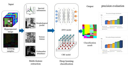
2. Materials and Methods
2.1. Multiple Feature Extraction
2.1.1. Texture Features
2.1.2. Endmember Abundance Features
2.1.3. Morphological Profiles
2.2. Fusion Strategy
2.2.1. Decision Fusion
2.2.2. Probability Fusion
2.2.3. Stacking Fusion
2.3. Image Classification
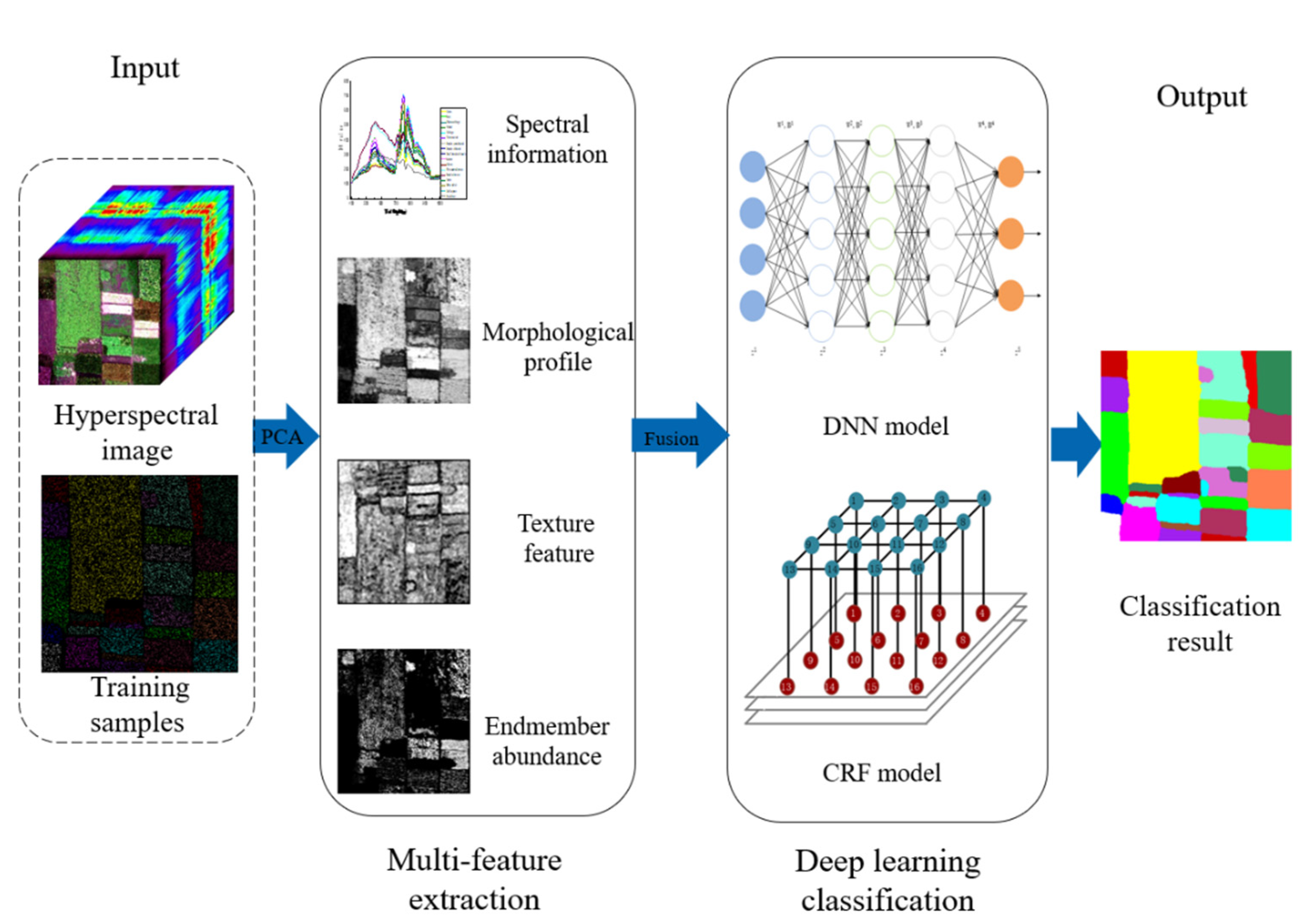
2.3.1. Deep Neural Networks
2.3.2. Conditional Random Field
3. Experiments
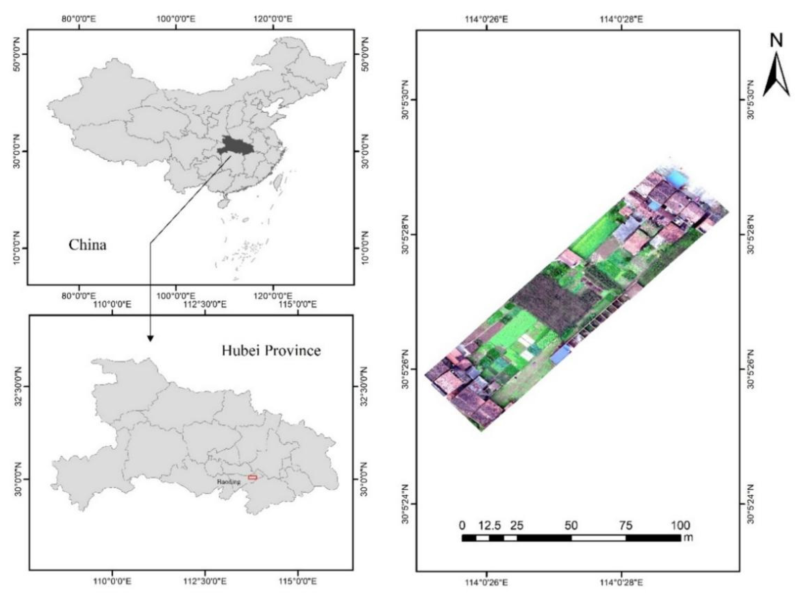
3.1. Experiential Data
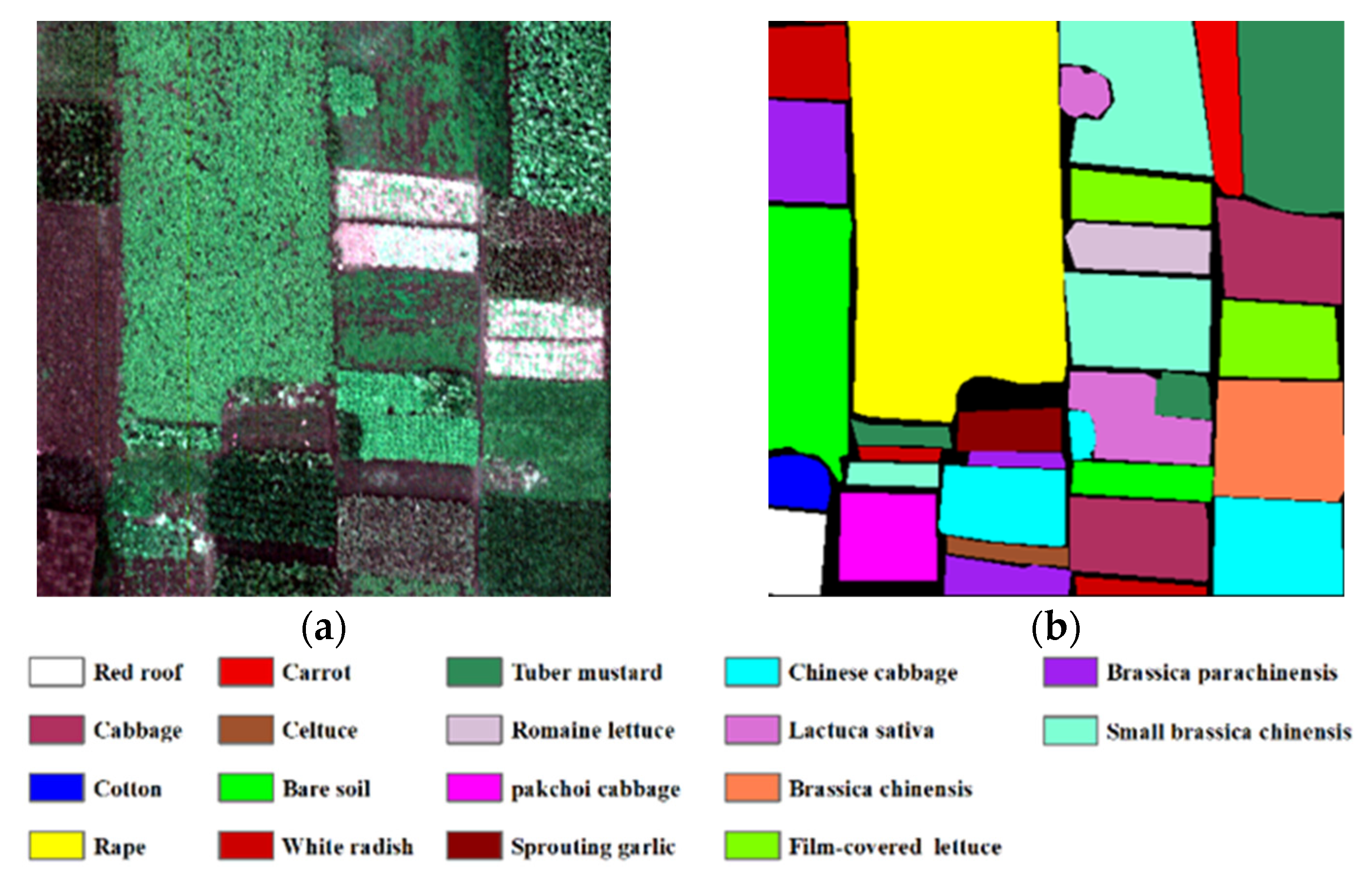
3.1.1. Honghu Dataset
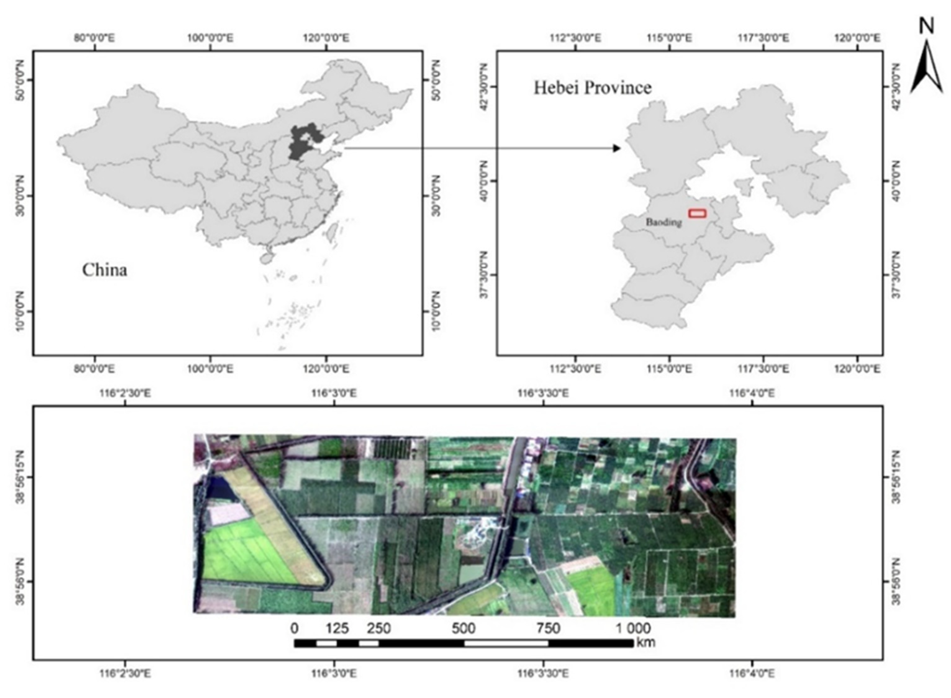
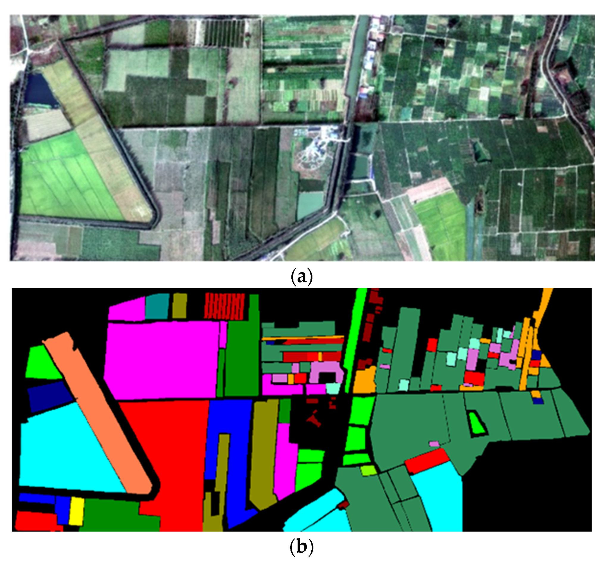
3.1.2. Xiong’an Dataset
3.2. Experiment Description
3.2.1. Experimental Setup
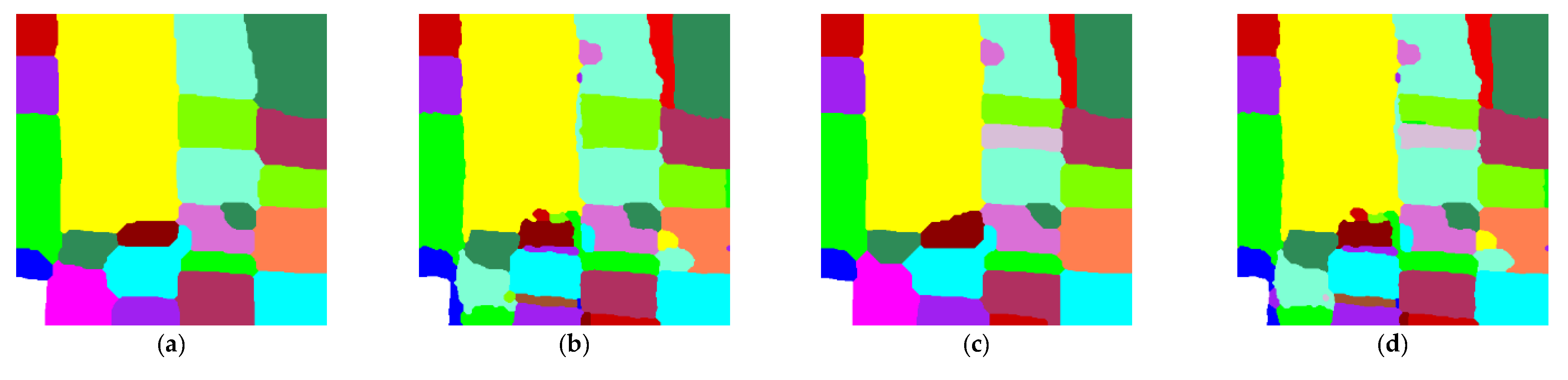
3.2.2. Experimental Results
3.3. Discussion
3.3.1. Effect of Sample Size
3.3.2. Effect of Classifier
3.3.3. Effect of CRF
4. Discussion
Author Contributions
Funding
Data Availability Statement
Acknowledgments
Conflicts of Interest
References
- Zhang, S.; Lei, Y.; Wang, L.; Li, H.; Zhao, H. Crop Classification Using MODIS NDVI Data Denoised by Wavelet: A Case Study in Hebei Plain, China. Chin. Geogr. Sci. 2011, 3, 68–79. [Google Scholar] [CrossRef]
- Prodhan, F.A.; Zhang, J.; Yao, F.; Shi, L.; Pangali Sharma, T.P.; Zhang, D.; Cao, D.; Zheng, M.; Ahmed, N.; Mohana, H.P. Deep Learning for Monitoring Agricultural Drought in South Asia Using Remote Sensing Data. Remote Sens. 2021, 13, 1715. [Google Scholar] [CrossRef]
- Yang, N. Application and development of remote sensing technology in geological disaster prevention and mineral exploration. Value Eng. 2020, 39, 242–243. [Google Scholar]
- Zhang, H.; Wang, L.; Tian, T.; Yin, J. A Review of Unmanned Aerial Vehicle Low-Altitude Remote Sensing (UAV-LARS) Use in Agricultural Monitoring in China. Remote Sens. 2021, 13, 1221. [Google Scholar] [CrossRef]
- Peng, X.; Han, W.; Ao, J.; Wang, Y. Assimilation of LAI Derived from UAV Multispectral Data into the SAFY Model to Estimate Maize Yield. Remote Sens. 2021, 13, 1094. [Google Scholar] [CrossRef]
- Bo, Y.; Liu, X. Object-Based Crop Species Classification Based on the Combination of Airborne Hyperspectral Images and LiDAR Data. Remote Sens. 2015, 7, 922–950. [Google Scholar]
- Pádua, L.; Marques, P.; Hruška, J.; Adão, T.; Peres, E.; Morais, R.; Sousa, J. Multi-Temporal Vineyard Monitoring through UAV-Based RGB Imagery. Remote Sens. 2018, 10, 1907. [Google Scholar] [CrossRef] [Green Version]
- Xiao, Z.; Gong, Y.; Long, Y.; Li, D.; Wang, X.; Liu, H. Airport Detection Based on a Multiscale Fusion Feature for Optical Remote Sensing Images. IEEE Geosci. Remote. Sens. Lett. 2017, 14, 1469–1473. [Google Scholar] [CrossRef]
- Lianze, T.; Yong, L.; Hongji, Z.; Sijia, L. Summary of UAV Remote Sensing Application Research in Agricultural Monitoring. Sci. Technol. Inf. 2018, 16, 122–124. [Google Scholar]
- Vincent, G.; Antin, C.; Laurans, M.; Heurtebize, J.; Durrieu, S.; Lavalley, C.; Dauzat, J. Mapping plant area index of tropical evergreen forest by airborne laser scanning. A cross-validation study using LAI2200 optical sensor. Remote. Sens. Environ. 2017, 198, 254–266. [Google Scholar] [CrossRef]
- Hinton, G.E.; Osindero, S.; Teh, Y.W. A fast learning algorithm for deep belief nets. Neural Comput. 2006, 18, 1527–1554. [Google Scholar] [CrossRef] [PubMed]
- Camps-Valls, G.; Bruzzone, L. Kernel-based methods for hyperspectral image classification. IEEE Trans. Geosci. Remote Sens. 2005, 43, 1351–1362. [Google Scholar] [CrossRef]
- Meyer, A.; Paglieroni, D.; Astaneh, C. K-means reclustering: Algorithmic options with quantifiable performance comparisons. In Optical Engineering at the Lawrence Livermore National Laboratory; International Society for Optics and Photonics: Bellingham, WA, USA, 2003; Volume 5001, pp. 84–92. [Google Scholar]
- Yi, C.; Nasrabadi, N.M.; Tran, T.D. Hyperspectral Image Classification via Kernel Sparse Representation. IEEE Trans. Geosci. Remote Sens. 2013, 51, 217–231. [Google Scholar] [CrossRef] [Green Version]
- Makantasis, K.; Karantzalos, K.; Doulamis, A.; Doulamis, N. Deep supervised learning for hyperspectral data classification through convolutional neural networks. In Proceedings of the 2015 IEEE International Geoscience and Remote Sensing Symposium (IGARSS), Milan, Italy, 26–31 July 2015; pp. 4959–4962. [Google Scholar] [CrossRef]
- He, K.; Zhang, X.; Ren, S.; Sun, J. Spatial Pyramid Pooling in Deep Convolutional Networks for Visual Recognition. IEEE Trans. Pattern Anal. Mach. Intell. 2015, 37, 1904–1916. [Google Scholar] [CrossRef] [Green Version]
- Galvao, L.S.; Formaggio, A.R.; Tisot, D.A. Discrimination of sugarcane varieties in Southeastern Brazil with EO-1 Hyperion data. Remote Sens. Environ. 2005, 94, 523–534. [Google Scholar] [CrossRef]
- Li, D.; Chen, S.; Chen, X. Research on method for extracting vegetation information based on hyperspectral remote sensing data. Trans. Chin. Soc. Agric. Eng. 2010, 26, 181–185. [Google Scholar]
- Bhojaraja, B.E.; Hegde, G. Mapping agewise discrimination of are canut crop water requirement using hyperspectral remote sensing. In Proceedings of the International Conference on Water Resources.Coastal and Ocean Engineering, Mangalore, India, 12–14 March 2015; pp. 1437–1444. [Google Scholar]
- Melgani, F.; Bruzzone, L. Classification of hyperspectral remote sensing images with support vector machines. IEEE Trans. Geosci. Remote Sens. 2004, 42, 1778–1790. [Google Scholar] [CrossRef] [Green Version]
- Tarabalka, Y.; Fauvel, M.; Chanussot, J.; Benediktsson, J.A. SVM- and MRF-Based Method for Accurate Classification of Hyperspectral Images. IEEE Geosci. Remote Sens. Lett. 2010, 7, 736–740. [Google Scholar] [CrossRef] [Green Version]
- Wei, L.; Yu, M.; Zhong, Y.; Zhao, J.; Liang, Y.; Hu, X. Spatial–Spectral Fusion Based on Conditional Random Fields for the Fine Classification of Crops in UAV-Borne Hyperspectral Remote Sensing Imagery. Remote Sens. 2019, 11, 780. [Google Scholar] [CrossRef] [Green Version]
- Liang, L.I.U.; Xiao-Guang, J.I.A.N.G.; Xian-Bin, L.I.; Ling-Li, T.A.N.G. Study on Classification of Agricultural Crop by Hyperspectral Remote Sensing Data. J. Grad. Sch. Chin. Acad. Sci. 2006, 23, 484–488. [Google Scholar]
- Wei, L.; Yu, M.; Liang, Y.; Yuan, Z.; Huang, C.; Li, R.; Yu, Y. Precise Crop Classification Using Spectral-Spatial-Location Fusion Based on Conditional Random Fields for UAV-Borne Hyperspectral Remote Sensing Imagery. Remote Sens. 2019, 11, 2011. [Google Scholar] [CrossRef] [Green Version]
- Li, C.H.; Kuo, B.C.; Lin, C.T.; Huang, C.S. A Spatial–Contextual Support Vector Machine for Remotely Sensed Image Classification. IEEE Trans. Geosci. Remote Sens. 2012, 50, 784–799. [Google Scholar] [CrossRef]
- Zhao, C.; Luo, G.; Wang, Y.; Chen, C.; Wu, Z. UAV Recognition Based on Micro-Doppler Dynamic Attribute-Guided Augmentation Algorithm. Remote Sens. 2021, 13, 1205. [Google Scholar] [CrossRef]
- Singh, J.; Mahapatra, A.; Basu, S.; Banerjee, B. Assessment of Sentinel-1 and Sentinel-2 Satellite Imagery for Crop Classification in Indian Region During Kharif and Rabi Crop Cycles. In Proceedings of the IGARSS 2019—2019 IEEE International Geoscience and Remote Sensing Symposium, Yokohama, Japan, 28 July–2 August 2019; pp. 3720–3723. [Google Scholar]
- Bai, J.; Xiang, S.; Pan, C. A Graph-Based Classification Method for Hyperspectral Images. IEEE Trans. Geosci. Remote Sens. 2013, 51, 803–817. [Google Scholar] [CrossRef]
- Ding, H.; Wang, X.; Wang, Y.; Luo, H. Ensemble Classification of Hyperspectral Images by Integrating Spectral and Texture Features. J. Indian Soc. Remote Sens. 2019, 47, 113–123. [Google Scholar] [CrossRef]
- AlSuwaidi, A.; Grieve, B.; Yin, H. Combining spectral and texture features in hyperspectral image analysis for plant monitoring. Meas. Sci. Technol. 2018, 29, 104001. [Google Scholar] [CrossRef] [Green Version]
- Wang, Y.; Yu, W.; Fang, Z. Multiple Kernel-Based SVM Classification of Hyperspectral Images by Combining Spectral, Spatial, and Semantic Information. Remote Sens. 2020, 12, 120. [Google Scholar] [CrossRef] [Green Version]
- Benediktsson, J.A.; Palmason, J.A.; Sveinsson, J.R. Classification of hyperspectral data from urban areas based on extended morphological profiles. IEEE Trans. Geosci. Remote Sens. 2005, 43, 480–491. [Google Scholar] [CrossRef]
- Xuan, H.; Qikai, L. Hyperspectral Image Classification Algorithm Based on Saliency Profile. Acta Opt. Sin. 2020, 40, 1611001. [Google Scholar] [CrossRef]
- Huang, X.; Guan, X.; Benediktsson, J.A.; Zhang, L.; Li, J.; Plaza, A.; Dalla Mura, M. Multiple Morphological Profiles from Multicomponent-Base Images for Hyperspectral Image Classification. IEEE J. Sel. Top. Appl. Earth Obs. Remote Sens. 2014, 7, 4653–4669. [Google Scholar] [CrossRef]
- Wang, Z.; Miao, X.; Huang, Z.; Luo, H. Research of Target Detection and Classification Techniques Using Millimeter-Wave Radar and Vision Sensors. Remote Sens. 2021, 13, 1064. [Google Scholar] [CrossRef]
- Licciardi, G.; Pacifici, F.; Tuia, D.; Prasad, S.; West, T.; Giacco, F.; Thiel, C.; Inglada, J.; Christophe, E.; Chanussot, J.; et al. Decision fusion for the classification of hyperspectral data: Outcome of the 2008 grs-s data fusion contest. IEEE Trans. Geosci. Remote Sens. 2009, 47, 3857–3865. [Google Scholar] [CrossRef] [Green Version]


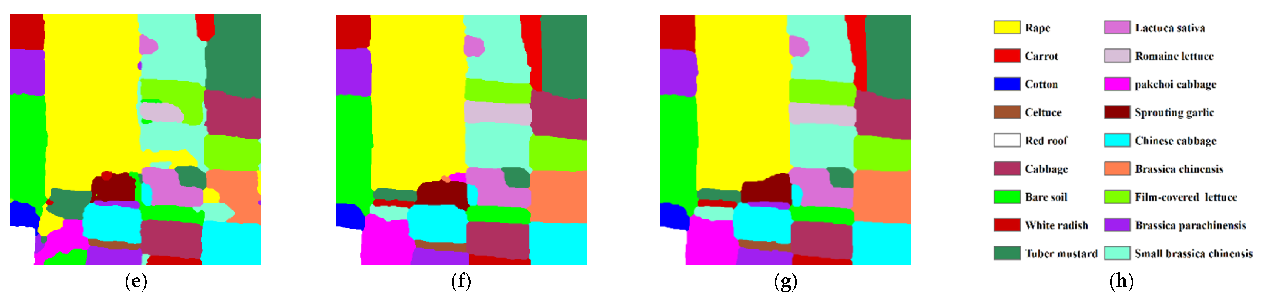
| Type | Pixel | Type | Pixel | Type | Pixel |
|---|---|---|---|---|---|
| roof | 66 | cabbage | 309 | celtuce | 30 |
| bare soil | 354 | tuber mustard | 343 | film-covered lettuce | 217 |
| cotton | 42 | brassica parachinensis | 189 | romaine lettuce | 90 |
| rape | 1137 | brassica chinensis | 217 | carrot | 83 |
| Chinese cabbage | 323 | small brassica chinensis | 477 | white radish | 122 |
| pakchoi cabbage | 121 | lactuca sativa | 158 | sprouting garlic | 61 |
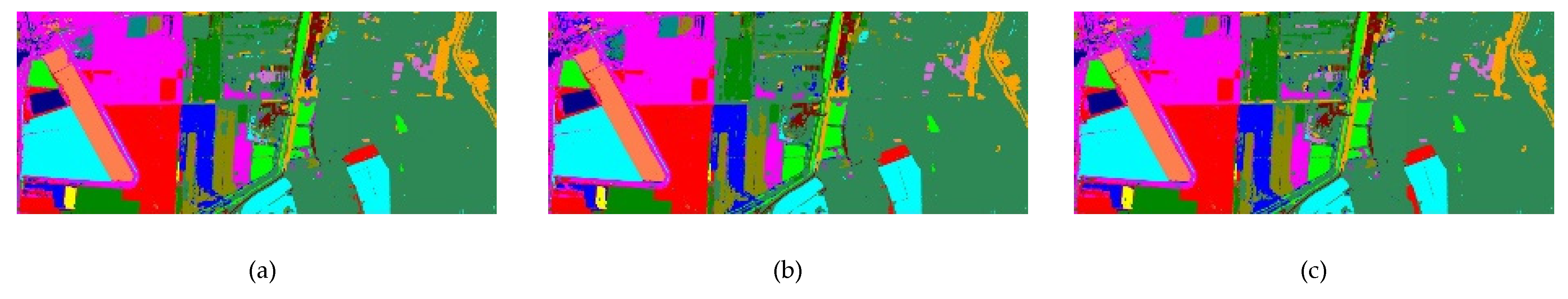
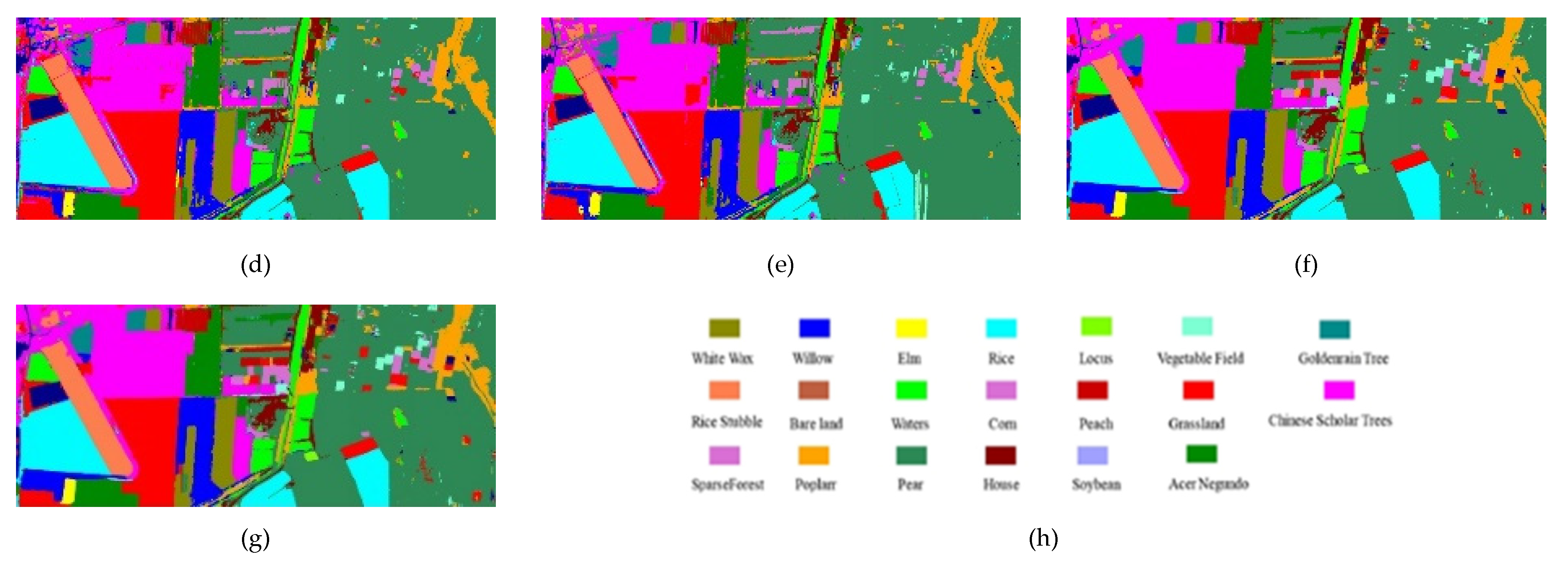
| Type | Pixel | Type | Pixel | Type | Pixel |
|---|---|---|---|---|---|
| rice | 135,662 | peach | 19,686 | koelreuteria paniculata | 6992 |
| water | 49,695 | corn | 17,750 | bare land | 11,523 |
| grassland | 126,569 | pear tree | 308,285 | rice stubble | 58,149 |
| acer compound | 67,695 | soybean | 2146 | locust | 1684 |
| willow | 54,384 | poplar | 27322 | sparse forest | 449 |
| sophora japonica | 142,827 | vegetable field | 8745 | house | 8885 |
| White wax | 50,834 | elm | 4606 |
| Types | Training Samples | Text Samples | Original Image | Endmember Abundance | GLCM Texture | Morphological Profiles | Decision Fusion | Probability Fusion | Stacking Fusion |
|---|---|---|---|---|---|---|---|---|---|
| Red roof | 66 | 2138 | 99.50 | 100.00 | 100.00 | 100.00 | 99.53 | 99.53 | 99.67 |
| Bare soil | 354 | 11,456 | 99.38 | 99.67 | 99.03 | 99.68 | 98.91 | 99.52 | 99.53 |
| Cotton | 42 | 1382 | 98.75 | 98.77 | 96.74 | 99.13 | 98.91 | 99.28 | 99.93 |
| Rape | 1137 | 36,783 | 100.00 | 99.58 | 100.00 | 99.72 | 99.31 | 99.96 | 99.83 |
| Chinese cabbage | 323 | 10,472 | 99.73 | 99.69 | 99.64 | 99.67 | 98.42 | 99.68 | 99.27 |
| Pakchoi cabbage | 121 | 3934 | 99.73 | 0.00 | 99.75 | 0.00 | 74.91 | 99.75 | 95.32 |
| Cabbage | 309 | 9998 | 99.89 | 99.95 | 99.92 | 99.95 | 99.54 | 99.88 | 99.97 |
| Tuber mustard | 343 | 11,098 | 90.10 | 98.59 | 99.20 | 98.57 | 96.27 | 98.13 | 98.88 |
| Brassica parachinensis | 189 | 6114 | 88.72 | 96.34 | 88.39 | 96.65 | 93.62 | 88.17 | 96.24 |
| Brassica chinensis | 217 | 7036 | 99.86 | 75.99 | 99.62 | 75.68 | 88.03 | 99.05 | 97.29 |
| Small brassica chinensis | 477 | 15,451 | 93.58 | 94.34 | 93.12 | 94.16 | 95.92 | 92.63 | 98.33 |
| Lactuca sativa | 158 | 5114 | 79.33 | 92.65 | 78.29 | 92.71 | 92.45 | 95.44 | 96.05 |
| Celtuce | 30 | 973 | 0.00 | 0.00 | 87.67 | 86.84 | 89.00 | 94.71 | 97.43 |
| Film-covered lettuce | 217 | 7046 | 99.65 | 99.52 | 99.29 | 98.85 | 97.39 | 99.87 | 99.45 |
| Romaine lettuce | 90 | 2921 | 0.00 | 0.00 | 99.65 | 90.96 | 91.34 | 95.52 | 95.31 |
| Carrot | 83 | 2710 | 0.00 | 94.32 | 78.65 | 94.32 | 90.00 | 98.38 | 96.64 |
| White radish | 122 | 3960 | 86.74 | 83.43 | 64.49 | 83.43 | 90.73 | 83.66 | 97.85 |
| Sprouting garlic | 61 | 2005 | 86.74 | 90.57 | 95.46 | 90.52 | 89.83 | 97.56 | 97.71 |
| OA | 91.05% | 91.77% | 91.92 | 93.64 | 95.98 | 96.89 | 98.71 | ||
| Kappa | 0.909 | 0.906 | 0.908 | 0.927 | 0.954 | 0.964 | 0.985 | ||
| Kappa | 0.9099 | 0.9065 | 0.9083 | 0.9277 | 0.9545 | 0.9649 | 0.9854 |
| Types | Training Samples | Text Samples | Original Image | Endmember Abundance | GLCM Texture | Morphological Profiles | Decision Fusion | Probability Fusion | Stacking Fusion |
|---|---|---|---|---|---|---|---|---|---|
| Rice | 135,662 | 316,544 | 98.40 | 98.21 | 98.28 | 74.58 | 98.60 | 98.83 | 99.95 |
| Waters | 49,695 | 115,955 | 92.46 | 93.74 | 93.87 | 94.19 | 97.16 | 96.61 | 99.72 |
| Grassland | 126,569 | 295,329 | 91.13 | 90.63 | 90.73 | 88.52 | 91.83 | 93.42 | 99.69 |
| Acer compound | 67,695 | 157,954 | 53.11 | 88.56 | 91.28 | 87.40 | 91.53 | 95.08 | 99.86 |
| Willow | 54,384 | 126,897 | 81.02 | 78.85 | 84.23 | 77.66 | 93.26 | 93.39 | 99.98 |
| Sophora japonica | 142,827 | 333,263 | 86.21 | 83.81 | 85.73 | 85.36 | 90.62 | 94.61 | 99.95 |
| White wax | 50,834 | 118,612 | 80.32 | 73.32 | 82.74 | 94.06 | 97.18 | 97.27 | 99.76 |
| Peach | 19,686 | 45,934 | 0.00 | 0.00 | 3.17 | 10.71 | 52.76 | 64.27 | 98.72 |
| Corn | 17,750 | 41,417 | 58.75 | 39.34 | 52.14 | 70.76 | 82.43 | 81.22 | 99.07 |
| Pear tree | 308,285 | 719,331 | 97.98 | 97.68 | 97.21 | 96.56 | 96.52 | 97.60 | 99.81 |
| Soybean | 2146 | 5007 | 0.00 | 0.00 | 12.36 | 53.55 | 54.61 | 35.97 | 98.24 |
| Poplar | 27,322 | 63,752 | 68.62 | 60.39 | 70.49 | 71.60 | 77.16 | 80.56 | 98.66 |
| Vegetable field | 8745 | 20,405 | 0.00 | 0.00 | 0.00 | 36.48 | 37.38 | 24.61 | 97.02 |
| Elm | 4606 | 10,748 | 88.49 | 74.78 | 85.64 | 83.41 | 86.95 | 90.69 | 98.68 |
| Koelreuteria Paniculata | 6992 | 16,314 | 95.69 | 95.65 | 94.84 | 95.42 | 99.35 | 98.62 | 99.91 |
| Bare land | 11,523 | 26,887 | 96.49 | 96.07 | 96.37 | 96.41 | 97.62 | 97.24 | 99.64 |
| Rice stubble | 58,149 | 135,682 | 96.95 | 96.90 | 96.86 | 97.50 | 98.99 | 98.71 | 99.97 |
| Locust | 1684 | 3929 | 0.00 | 0.00 | 0.00 | 17.29 | 64.89 | 0.00 | 98.07 |
| Sparse forest | 449 | 1048 | 0.00 | 0.00 | 0.00 | 0.83 | 50.31 | 0.00 | 88.84 |
| House | 8885 | 20,732 | 88.46 | 90.99 | 90.08 | 92.48 | 94.38 | 94.14 | 98.69 |
| OA | 88.86 | 87.46 | 88.85 | 89.17 | 89.34 | 92.74 | 99.71 | ||
| KAPPA | 0.836 | 0.846 | 0.863 | 0.885 | 0.888 | 0.910 | 0.995 |
| Honghu | Xiong’an | |||||
|---|---|---|---|---|---|---|
| Sample size | 3% | 5% | 10% | 3% | 5% | 10% |
| Original image | 91.05 | 91.85 | 92.32 | 88.86 | 90.78 | 91.71 |
| Decision Fusion | 95.98 | 96.39 | 96.87 | 89.34 | 91.67 | 93.26 |
| Probability Fusion | 96.89 | 97.22 | 97.51 | 92.74 | 93.26 | 94.92 |
| Stacking Fusion | 98.71 | 99.09 | 99.42 | 99.71 | 99.78 | 99.94 |
| Data | Accuracy | Decision Fusion | Probability Fusion | Stacking Fusion | |||
|---|---|---|---|---|---|---|---|
| SVM | DNN | SVM | DNN | SVM | DNN | ||
| Honghu | OA | 89.06% | 95.98% | 91.95% | 96.89% | 95.11% | 98.71% |
| Kappa | 0.875 | 0.908 | 0.908 | 0.954 | 0.946 | 0.985 | |
| Xiong’an | OA | 87.52% | 89.34% | 90.28% | 92.74% | 95.15% | 99.71% |
| Kappa | 0.845 | 0.915 | 0.903 | 0.928 | 0.929 | 0.995 | |
| Data | Accuracy | Decision Fusion | Probability Fusion | Stacking Fusion | |||
|---|---|---|---|---|---|---|---|
| Without CRF | With CRF | Without CRF | With CRF | Without CRF | With CRF | ||
| Honghu | OA | 89.89% | 95.98% | 92.76% | 96.89% | 94.91% | 98.71% |
| Kappa | 0.884 | 0.908 | 0.910 | 0.954 | 0.942 | 0.985 | |
| Xiong’an | OA | 88.72% | 89.34% | 91.03% | 92.74% | 91.56% | 99.71% |
| Kappa | 0.852 | 0.915 | 0.865 | 0.928 | 0.866 | 0.995 | |
Publisher’s Note: MDPI stays neutral with regard to jurisdictional claims in published maps and institutional affiliations. |
© 2021 by the authors. Licensee MDPI, Basel, Switzerland. This article is an open access article distributed under the terms and conditions of the Creative Commons Attribution (CC BY) license (https://creativecommons.org/licenses/by/4.0/).
Share and Cite
Wei, L.; Wang, K.; Lu, Q.; Liang, Y.; Li, H.; Wang, Z.; Wang, R.; Cao, L. Crops Fine Classification in Airborne Hyperspectral Imagery Based on Multi-Feature Fusion and Deep Learning. Remote Sens. 2021, 13, 2917. https://doi.org/10.3390/rs13152917
Wei L, Wang K, Lu Q, Liang Y, Li H, Wang Z, Wang R, Cao L. Crops Fine Classification in Airborne Hyperspectral Imagery Based on Multi-Feature Fusion and Deep Learning. Remote Sensing. 2021; 13(15):2917. https://doi.org/10.3390/rs13152917
Chicago/Turabian StyleWei, Lifei, Kun Wang, Qikai Lu, Yajing Liang, Haibo Li, Zhengxiang Wang, Run Wang, and Liqin Cao. 2021. "Crops Fine Classification in Airborne Hyperspectral Imagery Based on Multi-Feature Fusion and Deep Learning" Remote Sensing 13, no. 15: 2917. https://doi.org/10.3390/rs13152917