
The Impact of the Mesoscale Ocean Variability on the Estimation of Tidal Harmonic Constants Based on Satellite Altimeter Data in the South China Sea


Abstract
:1. Introduction
2. Data and Methods
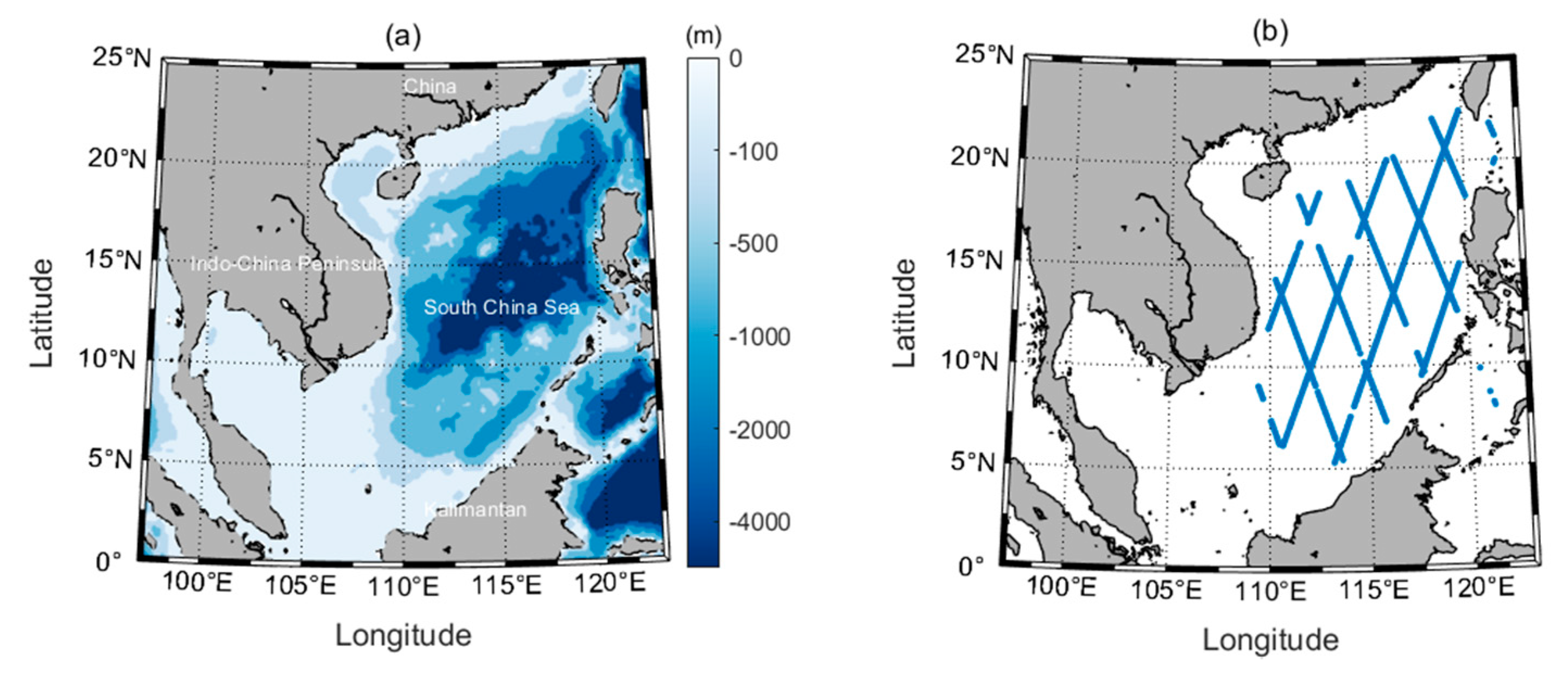
2.1. Altimetric Data
2.2. Tidal Aliasing in Altimetric Data
2.3. Tidal Harmonic Analysis
3. Results
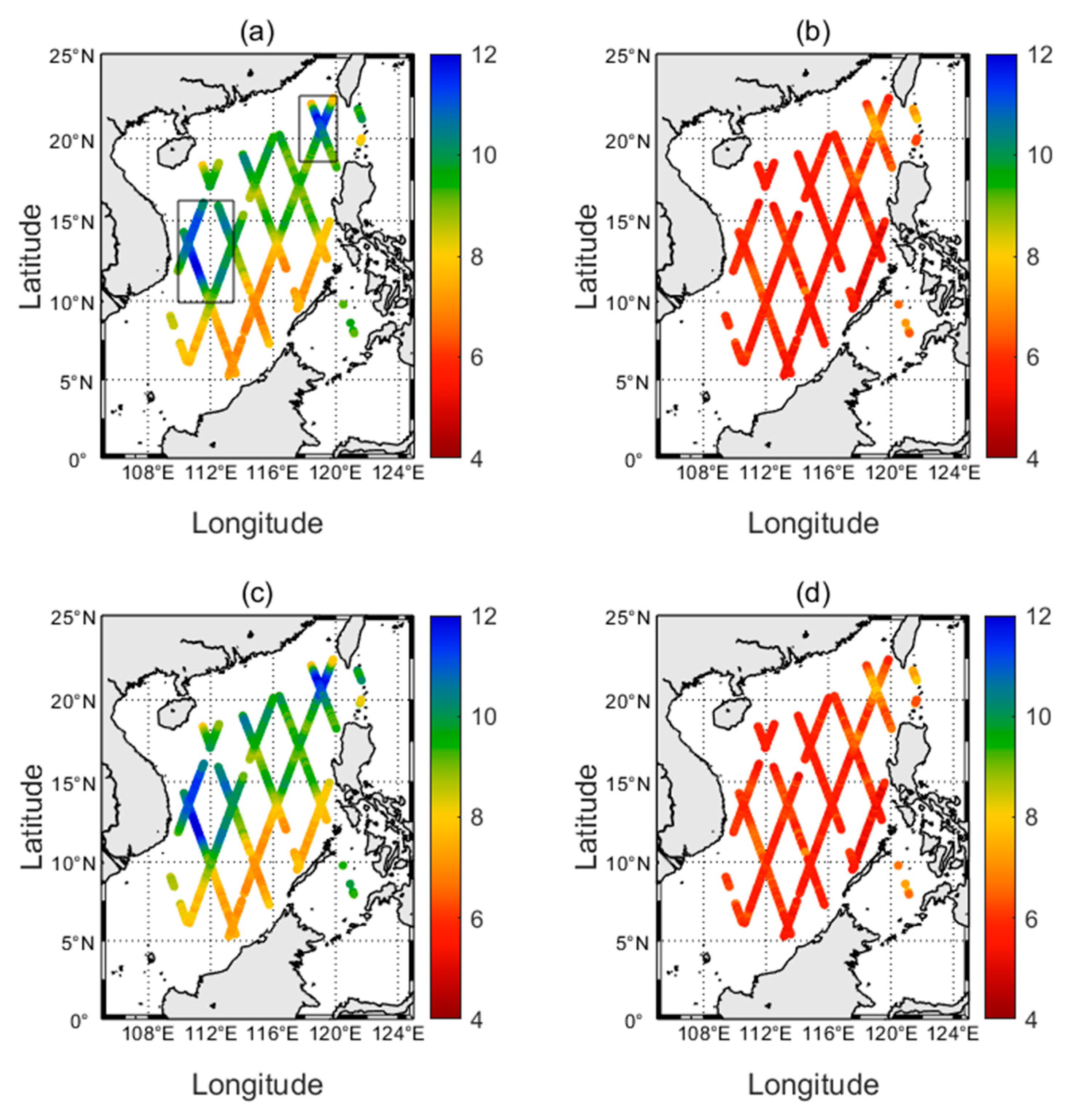
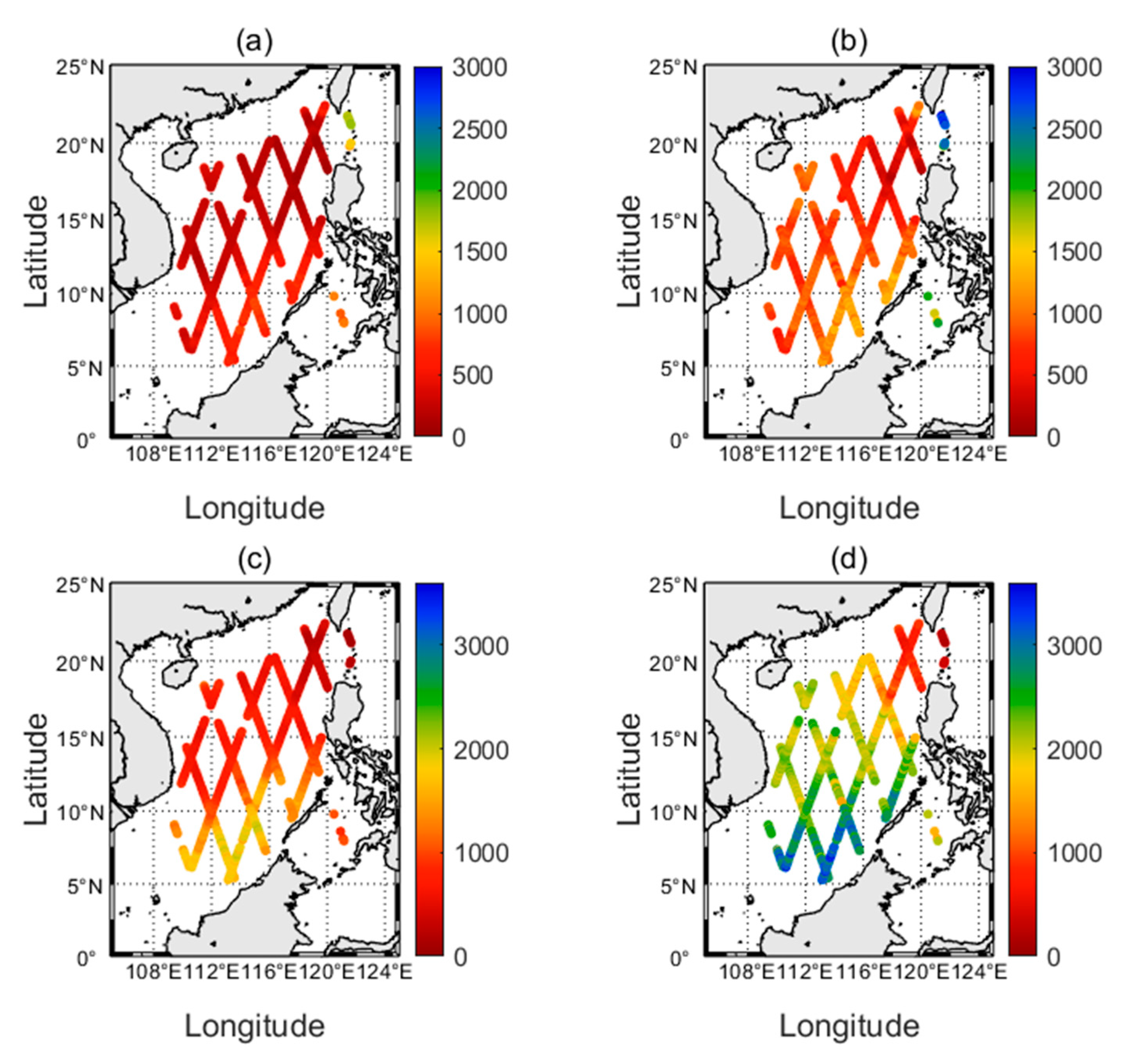
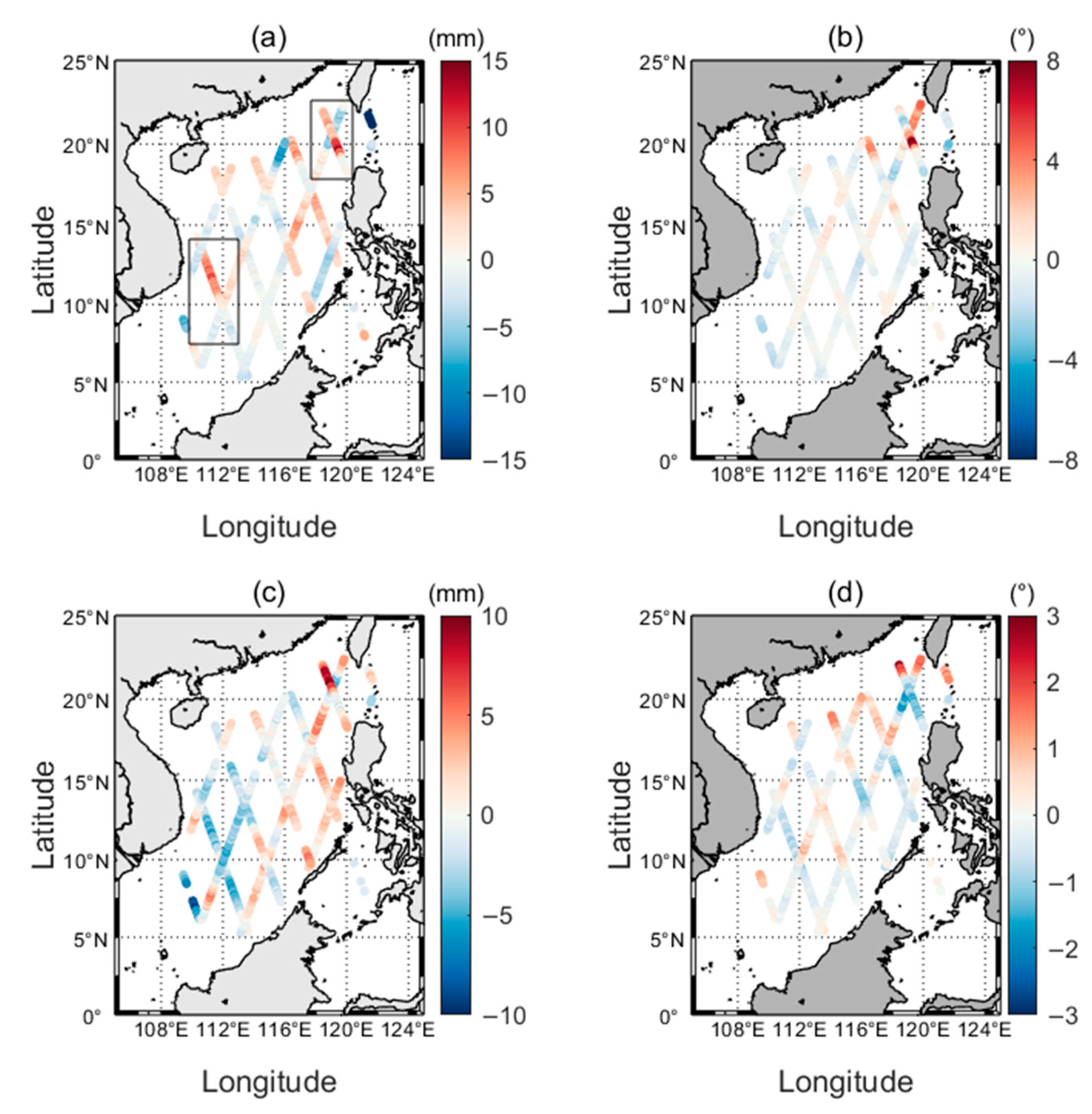
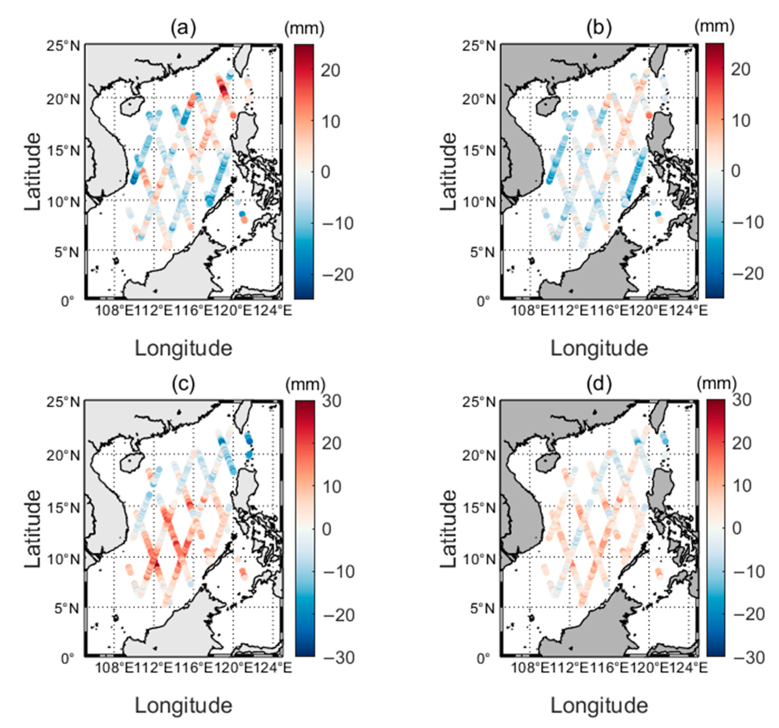
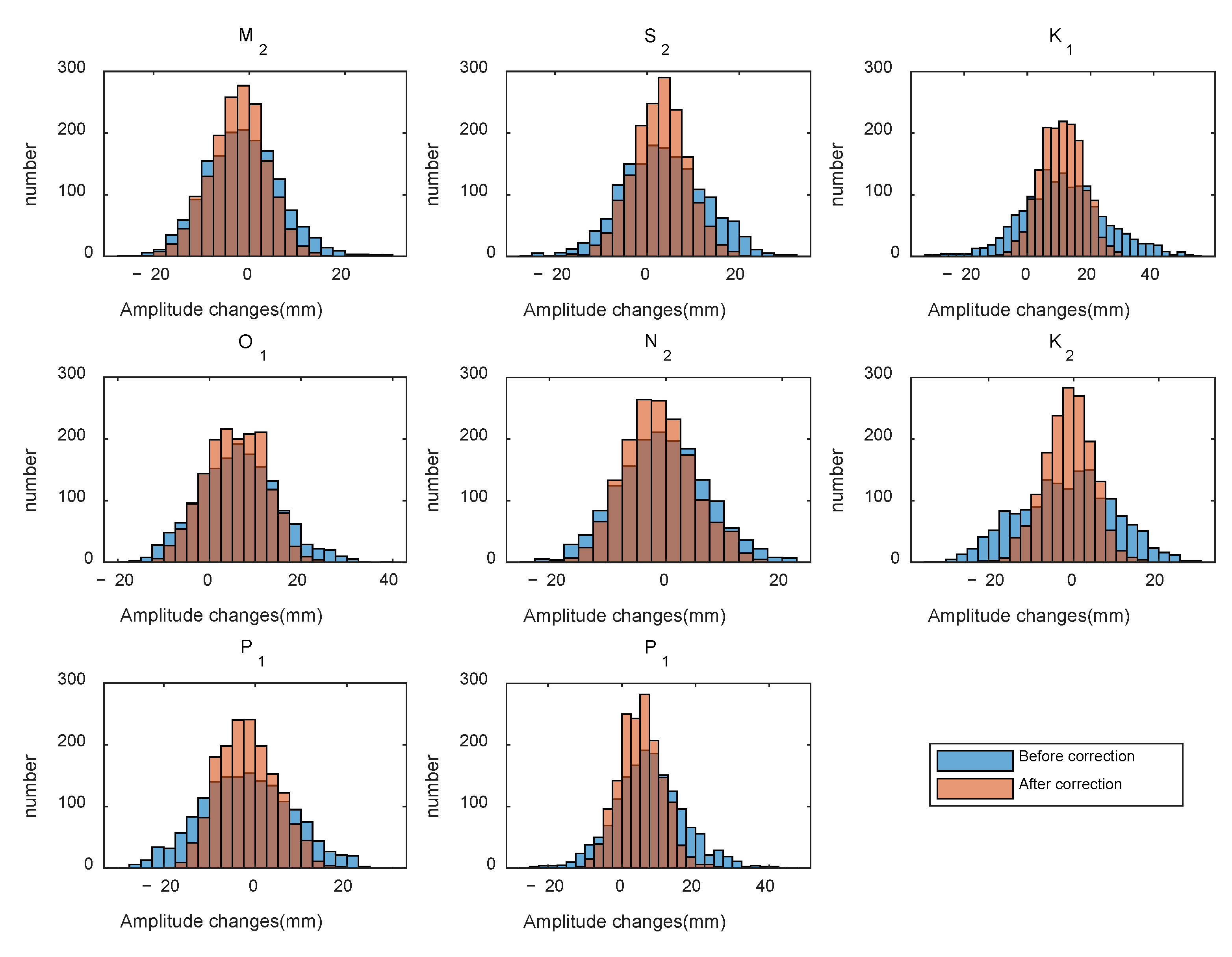
3.1. The Effect of MVC on the Estimation of Tidal Amplitude
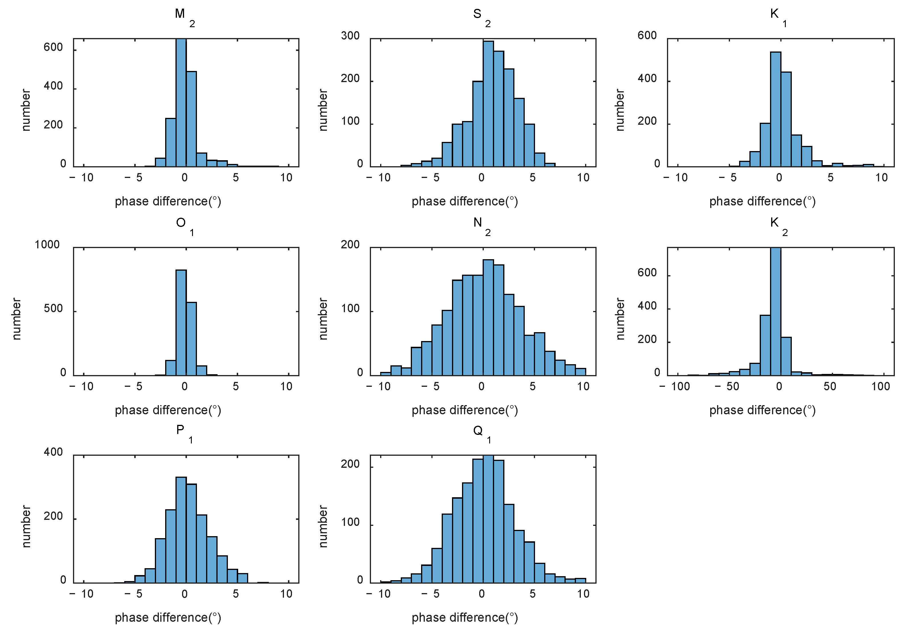
3.2. The Effect of MVC on the Estimation of Tidal Phase
3.3. Spatial Influence of Mesoscale Variability on Tidal Estimation
4. Discussion
4.1. Influence of Mesoscale Variability on the Estimation of Tidal Evolution
4.2. Tidal Evolution in the South China Sea
5. Summary and Conclusions
Supplementary Materials
Author Contributions
Funding
Data Availability Statement
Conflicts of Interest
Appendix A

| AD (mm) | <−10 | −10~−6 | −6~−2 | −2~2 | 2~6 | 6~10 | >10 |
|---|---|---|---|---|---|---|---|
| M2 | 12 | 45 | 293 | 743 | 413 | 82 | 12 |
| S2 | 0 | 2 | 432 | 843 | 287 | 36 | 0 |
| K1 | 44 | 175 | 397 | 569 | 277 | 88 | 50 |
| O1 | 2 | 19 | 419 | 791 | 342 | 26 | 1 |
| N2 | 0 | 13 | 312 | 1037 | 222 | 16 | 0 |
| K2 | 43 | 72 | 272 | 752 | 365 | 91 | 5 |
| P1 | 0 | 29 | 310 | 911 | 320 | 29 | 1 |
| Q1 | 0 | 43 | 336 | 814 | 391 | 16 | 0 |
| PD (°) | −90~−20 | −20~−9 | −7~−9 | −5~−7 | −3~−5 | −3~−1 | −1~1 | 1~3 | 3~5 | 5~7 | 7~9 | 9~20 | 20~90 |
|---|---|---|---|---|---|---|---|---|---|---|---|---|---|
| M2 | 0 | 0 | 0 | 0 | 3 | 293 | 1149 | 103 | 41 | 5 | 6 | 0 | 0 |
| S2 | 0 | 0 | 3 | 20 | 77 | 206 | 494 | 500 | 260 | 40 | 0 | 0 | 0 |
| K1 | 0 | 0 | 0 | 0 | 27 | 275 | 981 | 244 | 33 | 21 | 18 | 1 | 0 |
| O1 | 0 | 0 | 0 | 0 | 0 | 123 | 1396 | 81 | 0 | 0 | 0 | 0 | 0 |
| N2 | 0 | 6 | 27 | 97 | 181 | 306 | 338 | 300 | 171 | 105 | 41 | 28 | 0 |
| K2 | 164 | 437 | 149 | 171 | 186 | 138 | 94 | 57 | 44 | 37 | 31 | 33 | 41 |
| P1 | 0 | 0 | 0 | 6 | 68 | 368 | 640 | 358 | 128 | 30 | 2 | 0 | 0 |
| Q1 | 0 | 9 | 13 | 47 | 179 | 320 | 435 | 348 | 162 | 50 | 18 | 19 | 0 |
References
- Chao, B.F.; Ray, R.D. Oceanic Tidal Angular Momentum and Earth’s Rotation Variations. Prog. Oceanogr. 1997, 40, 399–421. [Google Scholar] [CrossRef]
- Munk, W.; Wunsch, C. The Moon, of Course. Oceanography 1997, 10, 132–134. [Google Scholar] [CrossRef]
- Francis, O.; Mazzega, P. Global Charts of Ocean Tide Loading Effects. J. Geophys. Res. 1990, 951, 11411–11424. [Google Scholar] [CrossRef]
- Desai, S.; Wahr, J.; Chao, Y. Error Analysis of Empirical Ocean Tide Models Estimated from TOPEX/POSEIDON Altimetry. J. Geophys. Res. 1997, 102, 25157–25172. [Google Scholar] [CrossRef]
- Tierney, C.; Parke, M.; Born, G. An Investigation of Ocean Tides Derived from Along-Track Altimetry. J. Geophys. Res. 1998, 103, 10273–10287. [Google Scholar] [CrossRef] [Green Version]
- Ray, R.; Byrne, D. Bottom Pressure Tides along a Line in the Southeast Atlantic Ocean and Comparisons with Satellite Altimetry. Ocean Dyn. 2010, 60, 1167–1176. [Google Scholar] [CrossRef] [Green Version]
- Xiu, P.; Chai, F.; Shi, L.; Xue, H.; Chao, Y. A Census of Eddy Activities in the South China Sea during 1993–2007. J. Geophys. Res. Ocean 2010, 115. [Google Scholar] [CrossRef] [Green Version]
- Dale, W.L. Wind and Drift Current in the South China Sea. Malay. J. Trop. Geogr. 1956, 8, 1–31. [Google Scholar]
- Cheng, Y.-H.; Ho, C.-R.; Zheng, Q.; Qiu, B.; Hu, J.; Kuo, N.-J. Statistical Features of Eddies Approaching the Kuroshio East of Taiwan Island and Luzon Island. J. Oceanogr. 2017, 73, 427–438. [Google Scholar] [CrossRef]
- Chen, G.; Hou, Y.; Chu, X. Mesoscale Eddies in the South China Sea: Mean Properties, Spatiotemporal Variability, and Impact on Thermohaline Structure. J. Geophys. Res. Ocean 2011, 116. [Google Scholar] [CrossRef]
- Yanagi, T.; Morimoto, A.; Ichikawa, K. Co-Tidal and Co-Range Charts for the East China Sea and the Yellow Sea Derived from Satellite Altimetric Data. J. Oceanogr. 1997, 53, 303–309. [Google Scholar]
- Yanagi, T.; Takao, T.; Morimoto, A. Co-Tidal and Co-Range Charts in the South China Sea Derived from Satellite Altimetry Data. La Mer 1997, 35, 85–93. [Google Scholar]
- Fang, G.; Kwok, Y.; Yu, K.; Zhu, Y. Numerical Simulation of Principal Tidal Constituents in the South China Sea, Gulf of Tonkin and Gulf of Thailand. Cont. Shelf Res. 1999, 19, 845–869. [Google Scholar] [CrossRef]
- Zu, T.; Gan, J.; Erofeeva, S.Y. Numerical Study of the Tide and Tidal Dynamics in the South China Sea. Deep-Sea Res. 2007, 55, 137–154. [Google Scholar] [CrossRef]
- Pan, H.; Lv, X.; Wang, Y.; Matte, P.; Chen, H.; Jin, G. Exploration of Tidal-Fluvial Interaction in the Columbia River Estuary Using S_TIDE. J. Geophys. Res. 2018, 123, 6598–6619. [Google Scholar] [CrossRef]
- Pascual, A.; Faugère, Y.; Larnicol, G.; Le Traon, P.Y. Improved Description of the Ocean Mesoscale Variability by Combining Four Satellite Altimeters. Geophys. Res. Lett. 2006, 33, 3–7. [Google Scholar] [CrossRef] [Green Version]
- Zaron, E.; Ray, R. Aliased Tidal Variability in Mesoscale Sea Level Anomaly Maps. J. Atmos. Ocean. Technol. 2018, 35. [Google Scholar] [CrossRef] [PubMed]
- Schlax, M.; Chelton, D. Aliased Tidal Errors in TOPEX/POSEIDON Sea Surface Height Data. J. Geophys. Res. Atmos. 1995, 99. [Google Scholar] [CrossRef]
- Fang, G.; Wang, Y.; Wei, Z.; Choi, B.; Wang, X.; Wang, J. Empirical Cotidal Charts of the Bohai, Yellow, and East China Seas from 10 Years of TOPEX/Poseidon Altimetry. J. Geophys. Res. 2004, 109. [Google Scholar] [CrossRef]
- Leffler, K.; Jay, D. Enhancing Tidal Harmonic Analysis: Robust (Hybrid L1/L2) Solutions. Cont. Shelf Res. 2009, 29, 78–88. [Google Scholar] [CrossRef]
- Pan, H.; Zheng, Q.; Lv, X. Temporal Changes in the Response of the Nodal Modulation of the M2 Tide in the Gulf of Maine. Cont. Shelf Res. 2019, 186, 13–20. [Google Scholar] [CrossRef]
- Pan, H.; Lv, X. Is There a Quasi 60-Year Oscillation in Global Tides? Cont. Shelf Res. 2021, 222, 104433. [Google Scholar] [CrossRef]
- Pawlowicz, R.; Beardsley, B.; Lentz, S. Classical Tidal Harmonic Analysis with Error Analysis in MATLAB Using T_TIDE. Comput. Geosci. 2002, 28, 929–937. [Google Scholar] [CrossRef]
- Anderson, K. Determination of Water Level and Tides Using Interferometric Observations of GPS Signals. J. Atmos. Ocean. Technol. 2000, 17, 1118–1127. [Google Scholar] [CrossRef]
- Wang, G.; Su, J.; Chu, P. Mesoscale Eddies in the South China Sea Observed with Altimeter Data. Geophys. Res. Lett. 2003, 30. [Google Scholar] [CrossRef] [Green Version]
- Li, J.; Zhang, R.; Jin, B. Eddy Characteristics in the Northern South China Sea as Inferred from Lagrangian Drifter Data. Ocean Sci. 2011, 7. [Google Scholar] [CrossRef]
- Liu, C.; Du, Y.; Zhuang, W.; Xia, H.; Xie, Q. Evolution and Propagation of a Mesoscale Eddy in the Northern South China Sea during Winter. Acta Oceanol. Sin. 2013, 32. [Google Scholar] [CrossRef]
- Zhang, M.; Von Storch, H.; Chen, X.; Wang, D.; Li, D. Temporal and Spatial Statistics of Travelling Eddy Variability in the South China Sea. Ocean Dyn. 2019, 69. [Google Scholar] [CrossRef] [Green Version]
- Egbert, G.; Bennett, A.F.; Foreman, M. TOPEX/POSEIDON Tides Estimated Using a Global Inverse Model. J. Geophys. Res. 1994, 99, 821–852. [Google Scholar] [CrossRef] [Green Version]
- Egbert, G.; Erofeeva, S. Efficient Inverse Modeling of Barotropic Ocean Tides. J. Atmos. Ocean. Technol. 2002, 19, 183–204. [Google Scholar] [CrossRef] [Green Version]
- Lyard, F.H.; Allain, D.J.; Cancet, M.; Carrère, L.; Picot, N. FES2014 Global Ocean Tide Atlas: Design and Performance. Ocean Sci. 2021, 17, 615–649. [Google Scholar] [CrossRef]
- Cartwright, D.; Ray, R. Oceanic Tides from Geosat Alimetry. J. Geophys. Res. Atmos. 1990, 95. [Google Scholar] [CrossRef]
- Godin, G. The Analysis of Tides; University of Toronto Press: Toronto, ON, Canada, 1972; p. 264. [Google Scholar]
- Parker, B. Tidal analysis and prediction. NOAA Special Publ. NOS CO-OPS 3; National Oceanic and Atmospheric Administration: Washington, DC, USA, 2007; p. 378.
- Pugh, D.; Woodworth, P. Sea-Level Science: Understanding Tides, Surges, Tsunamis and Mean Sea-Level Changes; Cambridge University Press: Cambridge, UK, 2012; p. 395. [Google Scholar]
- Ray, R.D. On Tidal Inference in the Diurnal Band. J. Atmos. Ocean. Technol. 2017, 34, 437–446. [Google Scholar] [CrossRef]
- Müller, M. Rapid Change in Semi-Diurnal Tides in the North Atlantic since 1980. Geophys. Res. Lett. 2011, 38. [Google Scholar] [CrossRef]
- Rodrıguez-Padilla, I.; Ortiz, M. On the Secular Changes in the Tidal Constituents in San Francisco Bay. J. Geophys. Res. Ocean. 2017, 122, 7395–7406. [Google Scholar] [CrossRef]
- Devlin, A.; Jay, D.; Zaron, E.; Talke, S.A.; Pan, J.; Lin, H. Tidal Variability Related to Sea Level Variability in the Pacific Ocean. J. Geophys. Res. Ocean. 2017. [Google Scholar] [CrossRef]
- Ray, R.D. Secular Changes of the M2 Tide in the Gulf of Maine. Cont. Shelf Res. 2006, 26, 422–427. [Google Scholar] [CrossRef] [Green Version]
- Müller, M.; Arbic, B.K.; Mitrovica, J.X. Secular Trends in Ocean Tides: Observations and Model Results. J. Geophys. Res. Ocean. 2011, 116, 1–19. [Google Scholar] [CrossRef] [Green Version]
- Ku, L.; Greenberg, D.; Garrett, C.; Dobson, F. Nodal Modulation of the Lunar Semidiurnal Tide in the Bay of Fundy and Gulf of Maine. Science 1985, 230, 69–71. [Google Scholar] [CrossRef]
- Flick, R.E.; Murray, J.F.; Ewing, L.C.; Asce, M. Trends in United States Tidal Datum Statistics and Tide Range. J. Waterw. Port Coast. Ocean Eng. 2003, 129, 155–164. [Google Scholar] [CrossRef] [Green Version]
- Woodworth, P.L.; Shaw, S.M.; Blackman, D.L. Secular Trends in Mean Tidal Range around the British Isles and along the Adjacent European Coastline. Geophys. J. Int. 1991, 104, 593–609. [Google Scholar] [CrossRef]
- Woodworth, P. A Survey of Recent Changes in the Main Components of the Ocean Tide. Cont. Shelf Res. 2010, 30, 1680–1691. [Google Scholar] [CrossRef] [Green Version]
- Colosi, J.; Munk, W. Tales of the Venerable Honolulu Tide Gauge*. J. Phys. Oceanogr. 2006, 36. [Google Scholar] [CrossRef]
- Guo, P.; Fang, W.; Liu, C.; Qiu, F. Seasonal Characteristics of Internal Tides on the Continental Shelf in the Northern South China Sea. J. Geophys. Res. 2012, 117, 4023. [Google Scholar] [CrossRef]
- Alford, M.; MacKinnon, J.; Nash, J.; Simmons, H.; Pickering, A.; Klymak, J.; Pinkel, R.; Sun, O.; Rainville, L.; Musgrave, R.; et al. Energy Flux and Dissipation in Luzon Strait: Two Tales of Two Ridges. J. Phys. Oceanogr. 2011, 41, 2211–2222. [Google Scholar] [CrossRef]
- Jan, S.; Chern, C.S.; Wang, J.; Chao, S.Y. Generation of Diurnal K1internal Tide in the Luzon Strait and Its Influence on Surface Tide in the South China Sea. J. Geophys. Res. 2007, 112. [Google Scholar] [CrossRef]
- Alford, M.; Peacock, T.; Mackinnon, J.; Nash, J.; Buijsman, M.; Centuroni, L.; Chao, S.-Y.; Chang, M.-H.; Farmer, D.; Fringer, O.; et al. The Formation and Fate of Internal Waves in the South China Sea. Nature 2015, 521, 65–69. [Google Scholar] [CrossRef]


| Constituent | Tidal Period (h) | Aliasing Period (Days) |
|---|---|---|
| M2 | 12.42 | 62.1 |
| S2 | 12.00 | 58.7 |
| K1 | 23.93 | 173.2 |
| O1 | 25.82 | 45.7 |
| N2 | 12.66 | 49.5 |
| K2 | 11.97 | 86.6 |
| P1 | 24.07 | 88.9 |
| Q1 | 26.87 | 69.4 |
| Constituent | M2 | S2 | K1 | O1 | N2 | K2 | P1 | Q1 |
|---|---|---|---|---|---|---|---|---|
| M2 | − | 2.97 | 0.27 | 0.47 | 0.67 | 0.60 | 0.56 | 1.63 |
| S2 | − | 0.24 | 0.56 | 0.86 | 0.50 | 0.47 | 1.05 | |
| K1 | − | 0.17 | 0.19 | 0.47 | 0.50 | 0.32 | ||
| O1 | − | 1.63 | 0.27 | 0.26 | 0.37 | |||
| N2 | − | 0.32 | 0.31 | 0.47 | ||||
| K2 | − | 9.18 | 0.95 | |||||
| P1 | − | 0.86 | ||||||
| Q1 | − |
| Constituent | Error before Correction (mm) | Error after Correction (mm) | SNR before Correction | SNR after Correction |
|---|---|---|---|---|
| M2 | 8.89 | 5.82 | 336.98 | 787.45 |
| S2 | 8.95 | 5.87 | 47.25 | 108.93 |
| K1 | 9.09 | 5.96 | 1114.32 | 2581.42 |
| O1 | 9.07 | 5.95 | 844.69 | 1963.79 |
| N2 | 8.89 | 5.82 | 14.35 | 33.04 |
| K2 | 8.99 | 5.89 | 4.39 | 10.26 |
| P1 | 8.96 | 5.87 | 113.07 | 263.48 |
| Q1 | 9.04 | 5.92 | 31.79 | 73.81 |
| Constituent | ||||||
|---|---|---|---|---|---|---|
| M2 | 116.9 | 15.2 | 12.97 | 139.2 | −10.3 | −7.43 |
| S2 | 33.0 | 6.0 | 18.16 | 33.4 | −4.9 | −14.65 |
| K1 | 177.5 | 16.2 | 9.13 | 95.3 | −12.7 | −13.36 |
| O1 | 185.9 | 10.4 | 5.59 | 320.9 | −10.0 | −3.12 |
| N2 | 19.0 | 6.7 | 35.24 | 35.3 | −8.2 | −23.22 |
| K2 | 11.9 | 11.4 | 95.99 | 20.8 | −13.5 | −64.79 |
| P1 | 80.0 | 11.0 | 13.78 | 36.1 | −4.3 | −11.88 |
| Q1 | 36.1 | 6.4 | 17.74 | 23.6 | −5.7 | −24.29 |
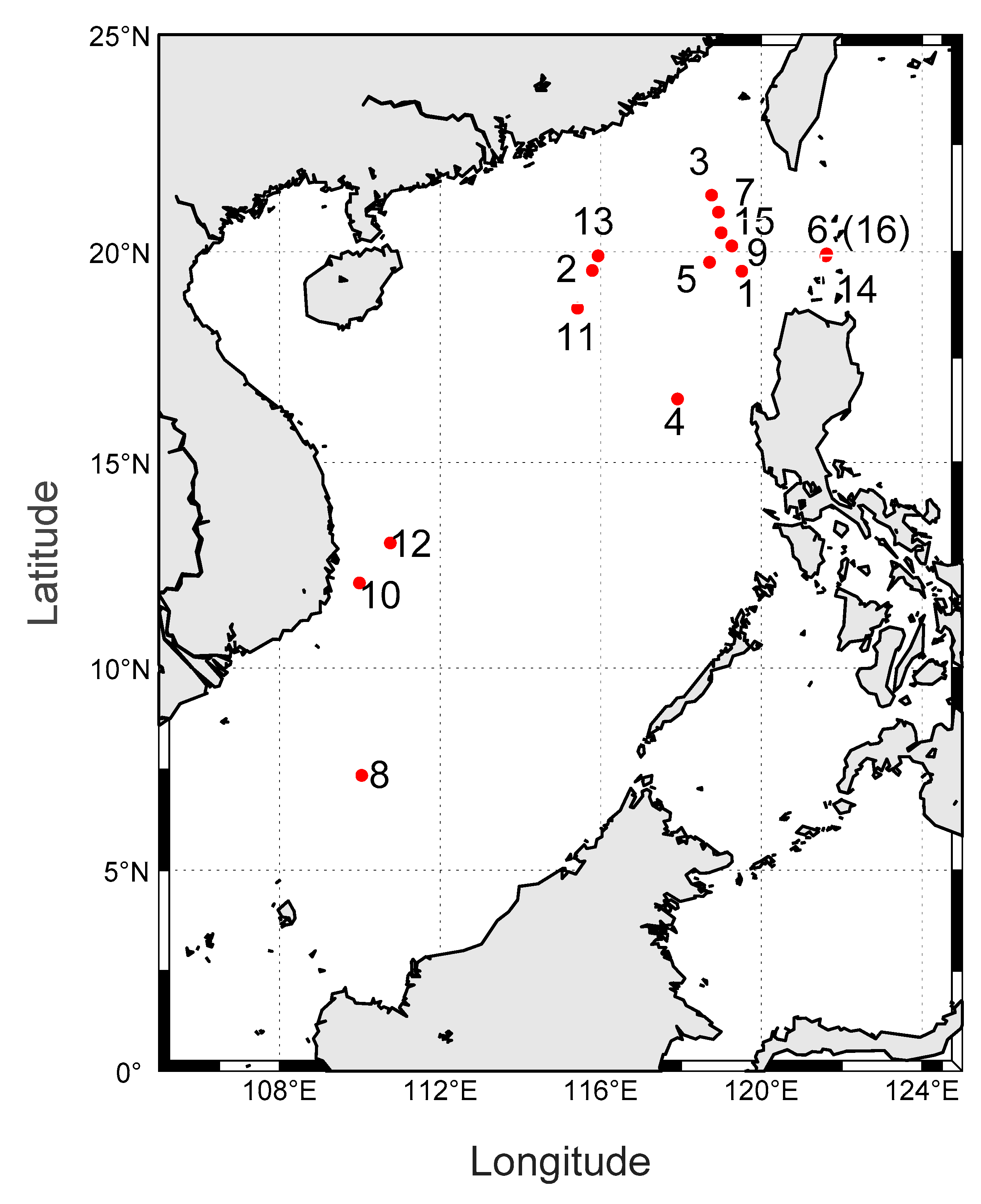
| Number | Constituent | Location (Lon, Lat) | Amplitude before Correction (mm) | Amplitude after Correction (mm) |
|---|---|---|---|---|
| 1 | M2 | (119.5127, 19.5467) | 101.8 | 116.9 |
| 2 | M2 | (115.7900, 19.5617) | 148.8 | 142.0 |
| 3 | S2 | (118.7611, 21.3209) | 40 | 47.4 |
| 4 | S2 | (117.9117, 16.5196) | 38.3 | 33.4 |
| 5 | K1 | (118.7081, 19.7563) | 161.3 | 177.5 |
| 6 | K1 | (121.6240, 19.9540) | 108.1 | 95.3 |
| 7 | O1 | (118.9299, 20.9271) | 175.5 | 185.9 |
| 8 | O1 | (110.0481, 7.3512) | 330.9 | 320.9 |
| 9 | N2 | (119.2644, 20.1387) | 12.3 | 19 |
| 10 | N2 | (109.9920, 12.0775) | 43.6 | 35.3 |
| 11 | K2 | (115.4216, 18.6728) | 0.5 | 11.9 |
| 12 | K2 | (110.7611, 13.0509) | 34.7 | 21.2 |
| 13 | P1 | (115.9345, 19.9070) | 69.0 | 80.0 |
| 14 | P1 | (121.6033, 19.9047) | 40.4 | 36.1 |
| 15 | Q1 | (118.9988, 20.4466) | 29.7 | 36.1 |
| 16 | Q1 | (121.6240, 19.9540) | 29.4 | 23.6 |
| Number | TPXO9 | FES2014 | ||||
|---|---|---|---|---|---|---|
| Amplitude from Model (mm) | The Error Rate before Correction (%) | The Error Rate after Correction (%) | Amplitude from Model (mm) | The Error Rate before Correction (%) | The Error Rate after Correction (%) | |
| 1 | 126.3 | 19.4 | 7.4 | 133.9 | 24.0 | 12.7 |
| 2 | 139.6 | −6.6 | −1.7 | 141.3 | −5.3 | −0.5 |
| 3 | 60.9 | 34.3 | 22.2 | 65.5 | 38.9 | 27.6 |
| 4 | 34.3 | −11.7 | 2.6 | 36.9 | −3.8 | 9.5 |
| 5 | 207.2 | 22.2 | 14.3 | 207.0 | 22.1 | 14.3 |
| 6 | 83.7 | −29.2 | −13.9 | 104.6 | −3.3 | 8.9 |
| 7 | 186.1 | 5.7 | 0.1 | 183.7 | 4.5 | −1.2 |
| 8 | 316.0 | −4.7 | −1.6 | 316.1 | −4.7 | −1.5 |
| 9 | 29.6 | 58.5 | 35.8 | 29.2 | 57.9 | 34.9 |
| 10 | 33.3 | −30.9 | −6.0 | 34.6 | −26.0 | −2.0 |
| 11 | 15.7 | 97.0 | 24.2 | 14.7 | 96.6 | 19.0 |
| 12 | 20.4 | −70.1 | −3.9 | 20.2 | −71.8 | −5.0 |
| 13 | 86.4 | 20.1 | 7.4 | 88.4 | 21.9 | 9.5 |
| 14 | 32.4 | −24.7 | −11.4 | 35.0 | −15.4 | −3.1 |
| 15 | 37.5 | 20.8 | 3.7 | 36.5 | 18.6 | 1.1 |
| 16 | 26.0 | −13.1 | 9.2 | 25.1 | −17.1 | 6.0 |
| Constituent | M2 | S2 | K1 | O1 | N2 | K2 | P1 | Q1 |
|---|---|---|---|---|---|---|---|---|
| Maximum PD (°) | 8.56 | 6.98 | 9.19 | 2.95 | 15.02 | 86.46 | 7.68 | 13.85 |
| Minimum PD (°) | −3.51 | −7.85 | −4.37 | −2.36 | −10.77 | −176.27 | −6.07 | −15.52 |
| Constituent | Maximum (mm) | Minimum (mm) | ||||
|---|---|---|---|---|---|---|
| Before Correction | After Correction | Difference | Before Correction | After Correction | Difference | |
| M2 | 29.7 | 16.2 | 13.5 | −26.7 | −25.3 | −1.4 |
| S2 | 32.5 | 21.2 | 11.3 | −25.7 | −17.8 | −7.9 |
| K1 | 52.7 | 29.5 | 23.2 | −32.3 | −11.0 | −21.3 |
| O1 | 39.1 | 24.9 | 14.2 | −17.8 | −15.6 | −2.2 |
| N2 | 22.3 | 17.5 | 4.8 | −23.9 | −20.5 | −3.4 |
| K2 | 28.6 | 17.0 | 11.6 | −32.6 | −21.7 | −10.9 |
| P1 | 28.1 | 23.4 | 4.7 | −27.6 | −17.8 | −9.8 |
| Q1 | 45.3 | 27.3 | 18 | −25.7 | −11.0 | −14.7 |
Publisher’s Note: MDPI stays neutral with regard to jurisdictional claims in published maps and institutional affiliations. |
© 2021 by the authors. Licensee MDPI, Basel, Switzerland. This article is an open access article distributed under the terms and conditions of the Creative Commons Attribution (CC BY) license (https://creativecommons.org/licenses/by/4.0/).
Share and Cite
Yu, Q.; Pan, H.; Gao, Y.; Lv, X. The Impact of the Mesoscale Ocean Variability on the Estimation of Tidal Harmonic Constants Based on Satellite Altimeter Data in the South China Sea. Remote Sens. 2021, 13, 2736. https://doi.org/10.3390/rs13142736
Yu Q, Pan H, Gao Y, Lv X. The Impact of the Mesoscale Ocean Variability on the Estimation of Tidal Harmonic Constants Based on Satellite Altimeter Data in the South China Sea. Remote Sensing. 2021; 13(14):2736. https://doi.org/10.3390/rs13142736
Chicago/Turabian StyleYu, Qian, Haidong Pan, Yanqiu Gao, and Xianqing Lv. 2021. "The Impact of the Mesoscale Ocean Variability on the Estimation of Tidal Harmonic Constants Based on Satellite Altimeter Data in the South China Sea" Remote Sensing 13, no. 14: 2736. https://doi.org/10.3390/rs13142736