The Response and Feedback of Ocean Mesoscale Eddies to Four Sequential Typhoons in 2014 Based on Multiple Satellite Observations and Argo Floats

Abstract

Four sequential tropical cyclones generated and developed in the Northwest Pacific Ocean (NWP) in 2014, which had significant impacts on the oceanic environment and coastal regions. Based on a substantial dataset of multiple-satellite observations, Argo profiles, and reanalysis data, we comprehensively investigated the interactions between the oceanic environment and sequential tropical cyclones. Super typhoon Neoguri (2014) was the first typhoon-passing studied area, with the maximum sustained wind speed of 140 kts, causing strong cold wake along the track. The location of the strongest cold wake was consistent with the pre-existing cyclonic eddy (CE), in which the average sea surface temperature (SST) cooling exceeded −5 °C. Subsequently, three tropical cyclones passed the ocean environment left by Neoguri, namely, the category 2 typhoon Matmo (2014), the tropical cyclone Nakri (2014) and the category 5 typhoon Halong (2014), which caused completely different subsequent responses. In the CE, due to the fact that the ocean stratification was strongly destroyed by Neoguri and difficult to recover, even the weak Nakri could cause a secondary response, but the secondary SST cooling would be overridden by the first response and thus could cause no more serious ocean disasters. If the subsequent typhoon was super typhoon Halong, it could cause an extreme secondary SST cooling, exceeding −8 °C, due to the deep upwelling, exceeding 700 m, surpassing the record of the maximum cooling caused by the first typhoon. In the anti-cyclonic eddy (AE), since the first typhoon Neoguri caused strong seawater mixing, it was difficult for the subsequent weak typhoons to mix the deeper, colder and saltier water into the surface, thus inhibiting secondary SST cooling, and even the super typhoon Halong would only cause as much SST cooling as the first typhoon. Therefore, the ocean responses to sequential typhoons depended on not only TCs intensity, but also TCs track order and ocean mesoscale eddies. In turn, the cold wake caused by the first typhoon, Neoguri, induced different feedback effects on different subsequent typhoons.

1. Introduction

Tropical cyclones (TCs) are strong natural hazards that are generated and developed in the tropical ocean. TCs with maximum wind speeds higher than 32.7 m/s in the north-western Pacific are referred to as typhoons, which are important for the local ocean environment [1,2,3], global ocean heat transport [4,5], and kinetic energy budget [6,7]. Air–sea interaction plays an important role in weather and climate change, and the interaction between tropical cyclones and ocean is an important part of air–sea interaction. Ocean response to typhoons has a long history of research, the most significant being the cold wake often seen along the typhoon track due to ocean surface enthalpy fluxes, vertical mixing, and upwelling [8,9,10]. Within the cold wake, there may also be marine phytoplankton blooms [11,12,13]. The SST cooling was usually by 1–6 °C [14,15,16], and by more than 10 °C in some extreme cases [17,18], which may have a negative feedback effect on the passing typhoon [19,20,21,22].

Most previous studies have focused on the research and analysis of the interaction between a single typical typhoon and the ocean [1,22,23,24]. In recent years, some studies have also focused on the interaction between the sequential typhoons and the ocean [16,25,26,27]. Yang et al. [25] studied the impact of two typhoons, Hagibis and Mitag, on the upper marine environment in the South China Sea (SCS) in 2007. Wu et al. [26] studied the response of the upper ocean to sequential typhoons Chan-Hom and Nangka in the SCS in 2015 and described the evolution of SST cooling under the influence of two sequential typhoons. Zhang et al. [27] used Moored Array to research the local current, temperature, and salinity during the passage of sequential typhoons Sarika and Haima in the SCS, and a 3D model was used to further study the internal ocean mechanisms. Some previous observations and simulations also show that the second TC usually cools the ocean surface cold wake of a preceding TC [26,28] and tends to be weakened as it travels over the cold wake of the first TC [29,30]. However, past research has only studied two sequential typhoons, and under these scenarios, we could not effectively compare the differences of the interaction between the subsequent typhoons with different categories and the first typhoon caused (FTC) ocean environment.

The sequential typhoons studied in the past almost occurred in the SCS, and the NWP is the region with a high frequency of typhoon genesis [31], accounting for more than twenty typhoons every year [32]. In addition, the NWP is also one of the most active mesoscale eddy regions, in which the Kuroshio has rich ocean dynamic characteristics, such as ubiquitous mesoscale eddy movement [33]. Due to the large-scale flow, typhoons generated in the NWP tend to move northwestwards, and the landfalling typhoons will cross the Kuroshio.

Although some sequential typhoons have been studied, some important issues remained unclear. For example, suppose that there are two TCs: one weaker and one stronger. There might be two different situations: first, a weaker TC with a sequential stronger TC; second, a stronger TC with a sequential weaker TC. Does the ocean have a similar response under such a different TC track order? In this paper, four sequential TCs with different categories in the NWP in 2014 were studied. Based on multi-platform satellite remote sensing observations, Argo observations and reanalysis data, we explored the different responses and feedbacks of the FTC ocean environment to subsequent typhoons with different categories. We compared the different oceanic responses due to stronger and weaker sequential TC. Furthermore, we also compared the different oceanic responses within CE and AE due to sequential TC. It was expected that the ocean responses to sequential typhoons depended on not only TCs intensity, but also TCs track order and ocean mesoscale eddies.

The remainder of this paper is organized as follows. In Section 2, we introduce the dataset and methodology; the third section presents the results, the fourth section presents the discussion and the last section concludes the study.

2. Materials and Methods

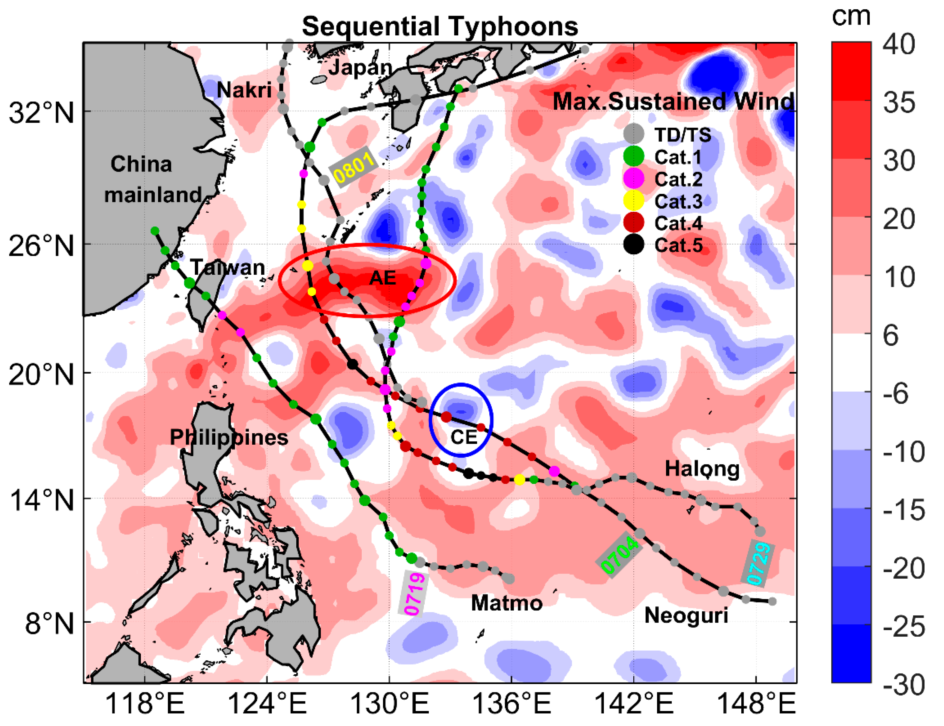
2.1. Typhoon Track Data

The “best track data” of the typhoon were obtained from the Joint Typhoon Warning Center (JTWC). Each best-track file contains the tropical cyclone center locations, the central pressures, and the maximum sustained wind (MSW) speeds. Figure 1 shows the tracks of the four sequential TCs, Neoguri, Matmo, Nakri and Halong, and the background SSHA field. According to the distribution of Argo float observations, we extracted a CE (shown as a blue cycle) and an AE (shown as a red cycle) as the research eddies. Typhoon Neoguri was generated in the NWP on 3 July 2014 and developed into a category 1 typhoon on 4 July 2014. It reached the MSW of 140 kts when passing the AE region from July 5 to 7. Typhoon Matmo was generated in the southeast of the Philippine Sea on July 18 and reached typhoon intensity on July 19, and gradually intensified to the MSW speed of 85 kts. It made landfall on Taiwan Island on July 22, and finally landed in Fujian on July 23. Nakri was generated in the NWP on July 30, and its maximum MSW speed was 40 kts. Typhoon Halong was generated on 28 July, then moved westward and gradually strengthened to a category 5 typhoon with the MSW speed of 140 kts.

2.2. Multiple Satellite Observations

The daily SST products were integrated with microwave and infrared optimally interpolated (MW_IR_OI) data from Remote Sensing Systems (RSS) (www.remss.com (accessed on 1 April 2021)). The MW_IR_OI data products used included the TRMM Microwave Imager, Advanced Microwave Scanning Radiomete, WindSat Polarimetric Radiometer and GPM microwave imager measured SST data. These instruments are suitable for analyzing the response of the upper ocean to the passage of typhoons as microwave imagers and radiometers are able to penetrate clouds, and the infrared channel of radiometers onboard polar-orbiting satellites has a high spatial resolution [34]. In this study, we used daily data with a spatial resolution of 9 × 9 km.

The daily SSHA and sea surface geostrophic velocity data with a spatial resolution of 0.25 × 0.25° were satellite altimeter data from the Ssalto/Duacs multisensor gridded delay-time altimetry product provided by Archiving, Validation and Interpretation of Satellite Oceanographic Data (AVISO) (http://marine.copernicus.eu (accessed on 1 April 2021)) and distributed by the Copernicus Marine and Environmental Monitoring Service. The oceanic dynamic features are defined as a positive-SSHA (AE) feature (closed contours, SSHA > 6 cm), negative-SSHA (CE) feature (closed contours, SSHA < −6 cm), and neutral condition (SSHA between −6 and 6 cm) [35] with a mononuclear eddy constraint [36].

The ocean color merged datasets were obtained from GlobColour (http://hermes.acri.fr/index.php?class=archive (accessed on 1 April 2021)). The GlobColour dataset provides daily, weekly, and monthly chlorophyll concentrations with a spatial resolution of 4, 25, and 100 km from 1997 to the present, and the sensors include single-sensor and merged products from SeaWiFS, MERIS, MODIS, VIIRS NPP, OLCI-A, VIIRS JPSS-1, and OLCI-B. Merged data products are coalesced from multiple mission observations into a single data product with better spatial and temporal coverage than the individual missions. In this study, we used daily and weekly ocean color data with a spatial resolution of 25 × 25 km.

The wind vector datasets included the wind at 10 m above the sea surface (SSW) from the Cross-Calibrated Multi-Platform (CCMP) gridded surface vector winds provided by RSS (www.remss.com (accessed on 1 April 2021)). The temporal resolution of the wind field data used is 6 h, and the spatial resolution is 0.25 × 0.25°.

The hourly infrared (IR) brightness temperature data were obtained from https://disc2.gesdisc.eosdis.nasa.gov/data/MERGED_IR/GPM_MERGIR.1/ (accessed on 1 April 2021). The spatial resolution of brightness temperature data is 4 × 4 km.

This study used the daily precipitation product with a spatial resolution of 0.1 × 0.1° from the Integrated Multi-satellite Retrievals for Global Precipitation Measurement mission (https://pmm.nasa.gov/data-access/downloads/gpm (accessed on 1 April 2021)).

2.3. Argo Profiles

We extracted the Argo float profiles from the real-time quality-controlled Argo database of the China Argo Real-time Data Center (http://www.argo.org.cn (accessed on 1 April 2021)). Argo is an array of 3887 active profiling floats, distributed almost uniformly across the global ocean, which provide temperature and salinity profiles from the surface to 2000 m depth. The array has approximately one float for every 3° of latitude and longitude and provides accurate and comprehensive measurements of changes to ocean temperature and salinity, enabling systematic assessments of the physical state of the upper ocean. The Argo data are collected and made freely available by the International Argo Project and the national programs that contribute to it. In this study, three groups of Argo (2902384, 2902493 and 2902500) in AE and two groups of Argo (2901524 and 5904304) in CE were selected during the passage of the sequential typhoon in 2014.

2.4. Reanalysis Data

A reanalysis dataset of the three-dimensional daily ocean temperature, salinity and derived density was extracted from the Global Ocean Forecasting System (GOFS) 3.1 reanalysis product based on the Hybrid Coordinate Ocean Model (HYCOM, http://apdrc.soest.hawaii.edu/ (accessed on 1 April 2021)). This dataset has a spatial resolution of 1/12 × 1/12° and 30 layers in the vertical direction.

ERA5 is the fifth generation ECMWF atmospheric reanalysis of the global climate (https://cds.climate.copernicus.eu/ (accessed on 1 April 2021)). It combines model data with observations from across the world into a globally complete and consistent dataset using the laws of physics. This dataset has a spatial resolution of 0.25 × 0.25° and a temporal resolution of 1 h.

2.5. Ekman Pumping

In order to measure the dynamic impact of typhoons on the ocean, we needed to calculate the upwelling velocity caused by Ekman pumping. The Ekman pumping velocity (EPV) caused by Ekman pumping can be calculated as follows [1]:

$$\mathrm{EPV}= \nabla \times \left(\mathit{\tau }/\mathit{\rho }\mathit{f}\right)$$

(1)

where ∇ is a gradient operator (total differential in all directions of space), called the Hamilton operator, f is the Coriolis parameter, $\mathit{\rho }$ is the density of seawater, and τ is the wind stress vector,

$$\mathit{\tau } = {\mathit{\rho }}_a{\mathit{C}}_D\left|U_{\mathbf{10}}\right|U_{\mathbf{10}}$$

(2)

$${\mathit{C}}_{\mathbf{D}}=\{\begin{array}{c}\left(\mathbf{4}-\mathbf{0.6}\left|{\mathbf{U}}_{\mathbf{10}}\right|\right)\times {\mathbf{10}}^{\mathbf{-}\mathbf{3}} \mathit{f}\mathit{o}\mathit{r} \left|U_{\mathbf{10}}\right|<\mathbf{5} \mathbf{m}/\mathbf{s}; \\ \left(\mathbf{0.737}+\mathbf{0.0525}\left|U_{\mathbf{10}}\right|\right)\times {\mathbf{10}}^{\mathbf{-}\mathbf{3}} \mathit{f}\mathit{o}\mathit{r} \mathbf{5}\mathbf{m}/\mathbf{s}\le \left|U_{\mathbf{10}}\right|<\mathbf{25} \mathbf{m}/\mathbf{s}\\ \mathbf{2.05}\times {\mathbf{10}}^{\mathbf{-}\mathbf{3}} \mathit{f}\mathit{o}\mathit{r} \left|U_{\mathbf{10}}\right|\ge \mathbf{25} \mathbf{m}/\mathbf{s} \end{array}$$

(3)

where ${\mathit{\rho }}_{\mathit{a}}$ is the air density, ${\mathit{C}}_{\mathbf{D}}$ is the drag coefficient [37,38] and $U_{\mathbf{10}}$ is the 10 m wind vector.

2.6. Eddy Detection

According to previous studies [39,40,41], the SSHA was used as the basis for the determination of mesoscale eddies [42,43]. One of the main purposes of this study was to explore the modulation mechanism of eddy dynamic features (a single eddy or eddy conglomeration) in the typhoon–ocean interaction. Therefore, we did not track a single eddy in this paper, and we identified AE and CE by the following criteria: if there was a series of closed contours in the SSHA field, when the value of the outermost closed contour was >6 cm, the region was defined as an AE; when the outermost closed contour was less than −6 cm, the region defined was a CE [44,45,46]. We identified the region of SSHA > 6 cm within the red ellipse as the AE conglomeration region, and the region of SSHA < −6 cm in the blue ellipse as the CE conglomeration region.

3. Results

Figure 2 shows the evolutions of the IR cloud top temperature (CTT); sea surface wind (SSW); Ekman pumping velocity (EPV); and rainfall filed during the passage of sequential typhoons Neoguri, Matmo, Nakri, and Halong. Figure 2a–d show that the IR CTT was lower than 190 K when sequential typhoons passed, which indicated that there was strong convection around the center of the typhoons. Figure 2e shows the strong SSW of 33.56 m/s and EPV over 1.2 × 10⁻³ m/s during the passage of the first typhoon, Neoguri. The EPV induced by Neoguri was distributed in a regular circle, and the EPV was positive (negative) within (beyond) the radius of 200 km from the center of the typhoon. The subsequent weak typhoons, Matmo and Nakri, caused relatively weak EPV, lower than 3 × 10⁻⁴ m/s. Compared with super typhoon Neoguri, the EPV induced by typhoon Matmo and Nakri was more dispersed, and the radius was wider than 300 km (Figure 2f–g). The last typhoon Halong was a category 5 typhoon, and it caused a strong EPV of 7 × 10⁻⁴ m/s; the EPV distribution was also a tight cycle similar to that of Neoguri (Figure 2h). Figure 2i–l show the rainfall distribution during the passage of sequential typhoons, and the maximum rainfall exceeded 200 mm/day. Figure 2i–j show that the rainfall induced by typhoon Neoguri and Matmo was stronger on the left-hand side of the track than on the right-hand side, which coincides with the findings of previous studies [46,47,48,49]. However, the subsequent typhoons, Nakri and Halong, induced a right-bias rainfall (Figure 2k–l), which was probably due to the asymmetrical precipitable water vapor distribution caused by the first two typhoons.

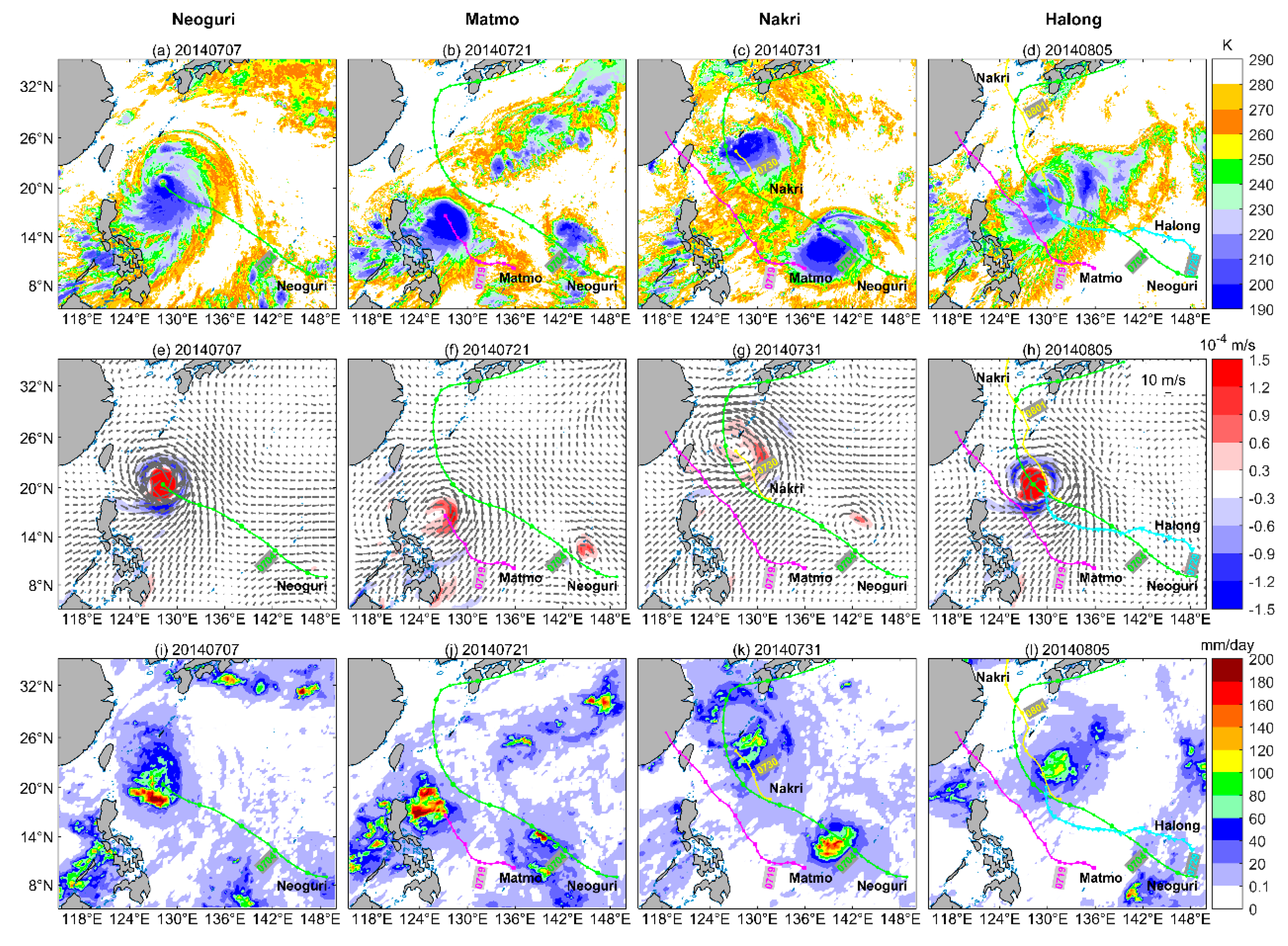
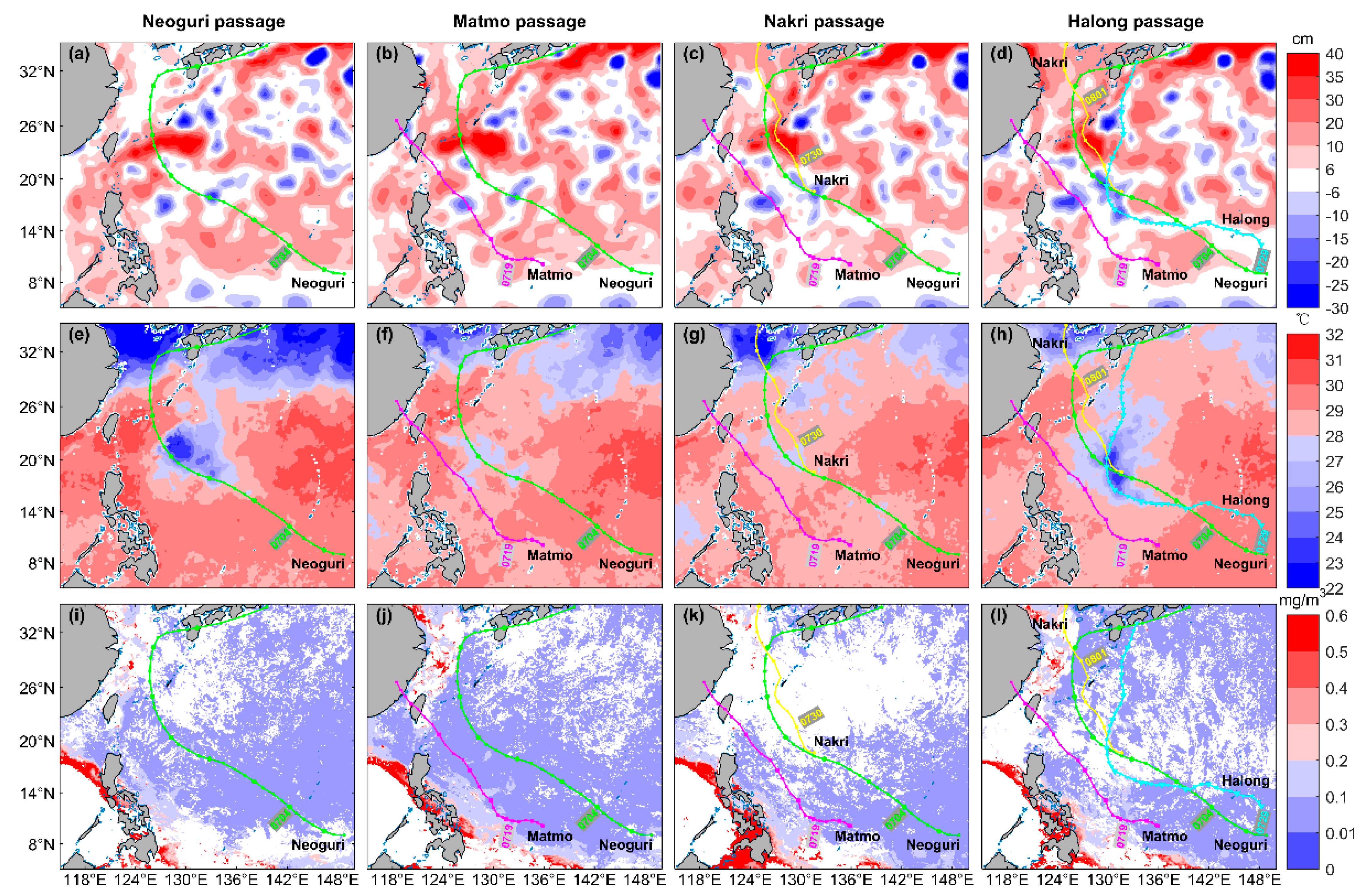
3.1. Surface Responses

Figure 3 shows the evolutions of SSHA, SST and chl-a concentration after the passage of each typhoon during four sequential typhoons. Figure 3a shows the background SSHA characteristics during the passage of Neoguri, and the eddy in the NWP was usually in the form of an irregular circle with the eddy area of AE. The target AE conglomeration and CE conglomeration were located just under the track of typhoon Neoguri. The area of CE conglomeration was small, and the area of AE conglomeration was larger. Influenced by the sequential typhoons, the CE conglomeration gradually strengthened and its area increased, while the AE conglomeration gradually weakened and its area decreased (Figure 3a–d).The more detail of eddies evolutions in Figure S1 in the Supplementary Material (SM). Before the passage of sequential typhoons, it was the hot summer season, and the SSTs in both the cold and warm eddies were close to 32 °C. Typhoon Neoguri caused a strong cold wake, which was significantly stronger on the right side of the track than the left (Figure 3e), which was caused by the better resonance of the wind stress and upper ocean current [1,50,51,52]. Figure 3f shows that typhoon Matmo induced SST cooling around the track, but the SST in the AE on the right side of the track hardly decreased. In contrast, the SST in the CE, which was far away from Matmo, caused a secondary cooling. Before the passage of TC Nakri, the SST almost recovered to higher than 28 °C. Although Nakri was weak, it caused SST cooling of 1–2 °C in the two CE regions on the south and north of AE during its passage, and the AE region blocked the spread of cooling (Figure 3g). As shown in Figure 3h, after typhoon Halong passed, a strong cold wake with a maximum SST cooling of over −8 °C was induced in the CE region, while the SST cooling was weak in the AE region. Therefore, the SST cooling in CE was stronger, while AE prevented the SST cooling from spreading northward (Figure 3e–h), which was consistent with previous studies [26,44,53]. Figure 3i–l show the evolutions of chl-a during the passage of sequential typhoons. Since the chl-a observation cannot penetrate the deep clouds during typhoons [23,54,55], we used the weekly averaged data to show the responses of chl-a concentration. In the tropical oceans, limited nutrient concentrations in the upper ocean are not conducive to enhancing primary productivity, which can be indicated by the variations in chl-a concentrations in phytoplankton [56,57]. Typhoon-induced upwelling and vertical mixing, which can be indicated by strong SST cooling, will bring relatively more phytoplankton and richer nutrients from the subsurface to the sea surface layer, and together with the usually sufficient sunshine and strong photosynthesis after the passing of a typhoon, there can be a marked increase in the surface chl-a concentration [12,58,59]. Figure 3i shows that typhoon Neoguri increased the chl-a concentration weakly in CE and caused no changes in AE. The chl-a concentration in the CE and AE hardly changed after the passage of Matmo and Nakri (Figure 3j–k). After the passage of typhoon Halong, the chl-a concentration in CE increased significantly with a maximum chl-a concentration of over 0.4 mg/m³.

We further quantitatively calculated the series of ocean responses to sequential typhoons in the CE and AE. As can be seen from Figure 4, during the passage of typhoon Neoguri, the average wind intensity in the CE and AE increased rapidly to 15–20 m/s (Figure 4a). The average SST cooling in the CE region was close to −5 °C, and the SST cooling in the AE region was 3 °C (Figure 4c). The average chl-a concentration in the CE increased by approximately 0.01 mg/m³, while that in the AE remained unchanged (Figure 4d). During the passage of subsequent typhoons Matmo and Nakri, the average wind speed of typhoons in the CE and AE was almost equal (Figure 4a). Figure 4b shows that there was almost no secondary cooling in the AE region, and the average SST cooling of 1–2 °C occurred in the CE region, but this cooling was overridden by the strong SST cooling caused by the first typhoon Neoguri. In addition, the chlorophyll concentration in CE and AE barely changed during Matmo and Nakri (Figure 4d). When the last typhoon Halong passed, the average SST cooling in CE was close to −6 °C, and the maximum SST cooling exceeded −8 °C, which surpassed the maximum SST cooling caused by the first typhoon Neoguri (Figure 4c). However, the maximum cooling in the AE was less than the SST cooling of −3 °C caused by Neoguri. The mean values of chl-a in AE and CE in Figure 4d were, respectively, calculated by the averaged satellite effective values of chl-a on all SSHA > 6 cm grids within the red ellipse and the averaged satellite effective values of chl-a on all SSHA < −6 cm grids within the blue ellipse. Figure 4d shows that the chl-a concentration generally increased within 3–7 days after typhoons. During the passage of typhoon Halong, the average chl-a concentration in the CE increased by 0.04 mg/m³ with a maximum chl-a concentration of more than 0.4 mg/m³. In conclusion, the first super typhoon, Neoguri, induced important impacts on the biophysical environment in the CE and AE, and different category subsequent typhoons caused different subsequent biophysical responses. After the super typhoon Neoguri, in the CE, as the ocean layer was completely destroyed and difficult to recover, even the distant subsequent typhoon Matmo or the weak subsequent TC Nakri could cause a secondary SST cooling, but the secondary SST cooling would be overridden by the SST cooling caused by the first typhoon, and would not cause more serious ocean disaster. If the subsequent typhoon was the super typhoon Halong, the secondary SST cooling in the CE would surpass the record of the maximum SST cooling and the blooming of chl-a concentration caused by the first typhoon. In the AE, the subsequent weak typhoons, Matmo and Nakri, could not cause a secondary SST cooling. Even the subsequent super typhoon Halong could only cause SST cooling comparable to that of the first typhoon. In the cases of sequential multiple typhoons, the intensity of subsequent typhoons and the characteristics of the ocean mesoscale eddy has a significant effect on the maximum damage degree of local ocean environment.

3.2. Subsurface and Deep Layer Responses

Based on multiple-satellite observations, the surface biophysical responses to four sequential typhoons were revealed, while the subsurface and deep ocean responses were not demonstrated. In particular, the difference in the surface response between CE and AE significantly depended on the three-dimensional ocean dynamic characteristics. Therefore, in order to better understand the physical mechanisms of the sequential typhoon–ocean interaction, and explain the surface phenomenon observed by satellite remote sensing, we studied the dynamic processes of subsurface ocean in the CE and AE through multiple Argo observations.

Figure 5 shows the detection time and relative positions of the two Argos in the CE. During the passage of typhoons Neoguri and Matmo, Argo 2901524 and 5904304 were located in the AE outside the CE. After the passage of typhoons, the area of the CE gradually increased and shifted westward, and Argos moved eastward at the same time; thus, they became closer (Figure 5a,b,e,f). Based on the temperature profiles observed by Argo, the mixed layer depth (MLD) was defined by a temperature threshold value of 0.2 °C [60,61]. The temperature profiles (Figure 6b,e) showed that the upper ocean temperature gradually decreased, and the MLD was shallower from 70.8 (black lines) to 30.2 m (blue lines). Nakri was generated in the north of the CE on July 29. Due to the weak wind and the distance from Argos, it did not affect the temperature and salinity profiles significantly. During the passage of typhoon Halong, both Argos were located in CE. Argo 2901524 was located on the right side of the typhoon track, and Argo 5904304 was located on the left side of the typhoon track. As shown by the temperature and salinity profiles in Figure 6, after typhoon Halong (the dark blue line), the upper ocean temperature decreased by more than 3 °C (Figure 6b,e), and the salinity increased significantly to more than 0.2 psu (Figure 6c,f). Additionally, we applied pre-typhoon and post-typhoon temperature profiles to calculate the upwelling distance [44,62]. The temperature profiles pre-typhoon and post-typhoon are T1(d) and T2(d), respectively, where d is the depth below the sea surface. If T1(d) = T2 (d–h), then the water at the depth of d has an upwelling height of h for temperature. In general, 1. during the passage of sequential typhoons, the temperature profiles detected by Argos in the CE were mainly upwelling, which was comprehensively performed as the “cold suction” effect [31,63]; 2. the upwelling distance detected by Argo 2901524 on the right side of the typhoon track exceeded 800 m, while the depth of seawater upwelling detected by Argo 5904304 on the left side was shallower than 400 m, which was consistent with the phenomenon of right-bias SST cooling [1].

Figure 7 shows the detection time and relative positions of the three Argos in the AE. During the passage of typhoon Neoguri, the three Argos were all located in the AE. As shown in Figure 8, Neoguri induced strong mixing during the passage of Neoguri (shallow black line), which cooled SST significantly, and the MLD deepened to 70 m. The salinity at Argo 2902384 increased, while that at Argo 2902493 and 2902500 decreased. As typhoon Matmo was far away from the AE, the temperature and salinity profiles detected by the three Argos were not changed. Nakri passed through the AE from July 30 to July 31, the three Argos were all located on the right side of Nakri track, and the distance was very close to the track. Nakri induced ocean mixing according to the temperature–salinity profiles before (dark blue line) and after Nakri (light red line). However, as the mixing caused by the first typhoon Neoguri was more intense, Nakri was unable to uplift the deeper, colder and saltier water, so it could not cause secondary cooling, and the salinity was also greatly reduced due to heavy precipitation. During the passage of the last typhoon, Halong, Argo 2902384 was located to the left side of the typhoon track, Argo 2902493 was just under the typhoon track, and Argo 2902500 moved into the CE area. At Argo 2902384, the MLD deepened, but the temperature did not decrease significantly, and the salinity did decrease significantly. At Argo 2902493, MLD deepened, and temperature and salinity decreased. In the CE, Argo 2902500 was mainly dominated by upwelling, and thus the temperature and salinity decreased. In general, 1. during the passage of sequential typhoons, the temperature profiles detected by Argos in the AE were mainly mixing, which was comprehensively performed as the “heat pump” effect [64]; 2. the strong oscillation of the water mass was related to the energy change inside the eddy and usually occurred near the minimum point of salinity. The depth of salinity oscillation in the AE was approximately 700 m based on the combination of all the Argo salinity profiles in Figure 8c,f,i, which was much deeper than that in the CE (Figure 6c,f), indicating that the energy of typhoons might be easily transported to the deeper layer in the AE.

The three-dimensional ocean dynamic characteristics in the CE and AE could be clearly demonstrated by sufficient Argo observations, which further explained the mechanism of sea surface responses to four sequential typhoons in the CE and AE. Secondary SST cooling in the CE was mainly caused by the upwelling of cold water, while secondary SST cooling in the AE needed to be induced by mixing. During the passage of the first super typhoon Neoguri, due to strong mixing and upwelling, significant surface cooling occurred in both the CE and AE, and the subsurface ocean was severely destroyed. After the passage of Neoguri, the upper ocean continued to upwell in the CE, and even the weak subsequent TC Nakri could further cause the upwelling of the cooler subsurface water; thus, the secondary SST cooling occurred. However, as the upwelling was weaker than that of Neoguri, the secondary SST cooling was significantly weaker than the first SST cooling. If the subsequent typhoon was super typhoon Halong, the upwelling in the CE was more intense under the addition of previous typhoons. Argo observations showed that the seawater upwelling depth exceeded 700 m, resulting in an extreme secondary SST cooling with the maximum cooling exceeding −8 °C, which surpassed the record of SST cooling caused by the first typhoon Neoguri. In the AE, since the first typhoon Neoguri had caused strong seawater mixing, the subsequent weak typhoons were difficult to upwell the deeper, colder and saltier water, so it was difficult to cause secondary SST cooling. Even if the super typhoon Halong followed, it would only cause SST cooling comparable to that of the first typhoon.

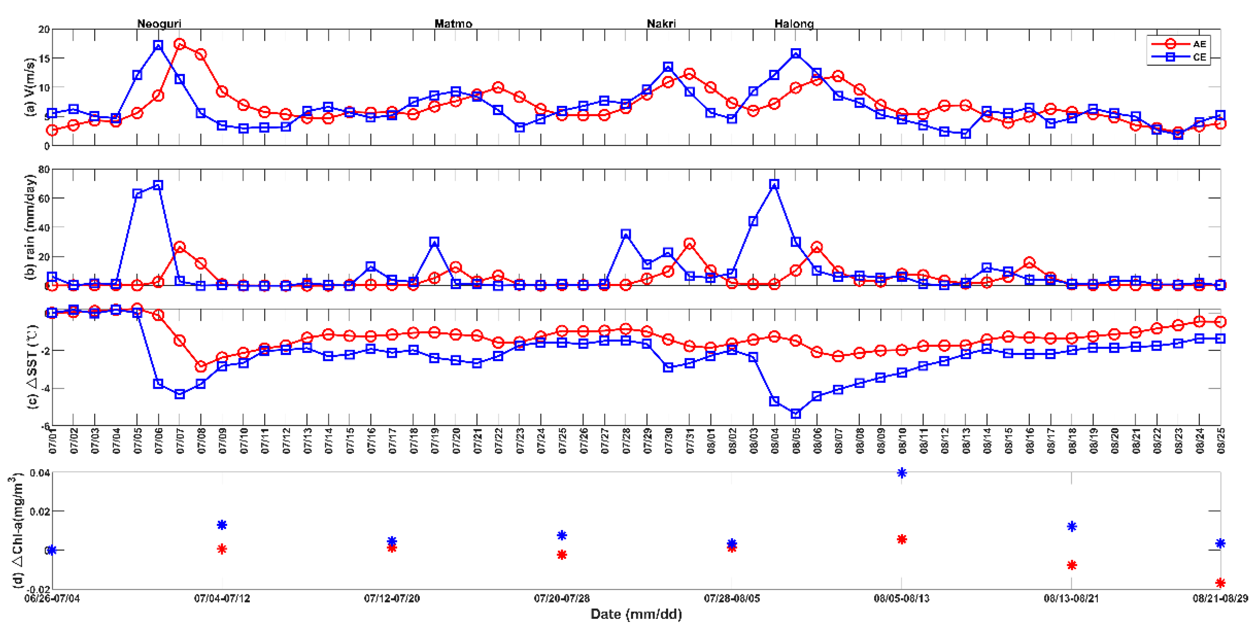
3.3. Ocean Feedbacks

We explored the feedback of FTC ocean environment after Neoguri on the different-category subsequent typhoons. Figure 9 shows the distributions of ocean heat content (OHC), sensible heat flux (SHL) and latent heat flux (LHF) during the passage of four sequential typhoons. OHC is defined as the heat content integrated from the surface down to 100 m, and the ocean temperature data used here were the reanalysis data from HYCOM. Figure 9a–d show that the NWP contained a high ocean heat content of higher than 1 × 10⁹ J/m², and the OHC decreased significantly around the track of typhoons. Especially in the CE, the strong upwelling caused by the typhoons led to a strong cooling of the water from the surface down to 100 m, further decreasing the OHC. The decrease in OHC in the AE was mainly caused by the strong surface heat flux from the ocean to the atmosphere during the passage of typhoons. It can be seen from Figure 9e–l that when a typhoon moves on the ocean, the ocean surface within the radius of the typhoon wind circle would transport a large amount of LHF and SHL to the typhoon, which is crucial for the maintenance and development of typhoons.

According to the Statistical Hurricane Intensity Prediction Scheme (SHIPS) [65,66]. In Figure 10, the evolutions of vertical wind shear (VWS, 200–850 hpa), relative humidity (RH) at 600 hPa, temperature at 200 hPa and relative vorticity at 850 hPa during four sequential typhoons were used to analyze the atmospheric and oceanic factors of typhoon intensity. According to Figure 10a–d, during the passage of the super typhoons Neoguri and Halong, the VWS around the typhoons was relatively weak and the strong wind shear area was small, while the wind shear around the typhoons Matmo and Nakri was strong, and the strong VWS area was large. Figure 10e–h show that the RH near the typhoon was high during the typhoon passage; in particular, the RH in the core of the super typhoons Neoguri and Halong was close to 100%, which was important to the maintenance and development of strong typhoons. Figure 10i–l show the 200 hPa temperature, which represented the tropopause temperature. The 200 hPa temperature in the center of typhoons was relatively low, and the high temperature area deviated from the center of the typhoon. Figure 10m–p show that the central vorticity of typhoons was a regular solid circle. The vorticity distribution of the super typhoons Neoguri and Halong was very compact, while the vorticity of the weak typhoon Matmo and TC Nakri was relatively weak and loose.

In order to further explore the dependence of subsequent TCs intensity on the ocean eddies and previous typhoons, the solid lines in Figure 11 show evolutions of the atmospheric and oceanic environments during four sequential typhoons, and the dotted lines show the environmental evolutions before each typhoon. As can be seen, after the passage of the first typhoon Neoguri, the local cold wake occurred, atmospheric humidity decreased, and the VWS strengthened, which were not in favor of the generation of subsequent typhoons. However, the local atmospheric environments recovered rapidly, all the three subsequent TCs generated once the environmental RH recovered and the VWS weakened below to 10 m/s. Compared with the local atmospheric environments, the oceanic environments were more stable and the cold wake and ocean eddies caused by the previous typhoon had a significant influence on the intensity of subsequent typhoons. To explore the modulation mechanism of ocean mesoscale eddies on the subsequent typhoons, the vertical dotted lines showed the periods when typhoon passing the CE (black dotted lines) and AE (red dotted lines). The eddy modulation mechanism on the subsequent TCs with different intensity was quiet different. When the subsequent typhoons were category 2 typhoon Matmo or TC Nakri, the FTC SST cooling suppressed the intensification of subsequent typhoons. When the subsequent typhoon was the category 5 typhoon Halong, the FTC SST cooling significantly weakened the intensity of typhoon.

4. Discussions

The response of ocean to tropical cyclones has been widely investigated in the past; in particular, the ocean response to individual typhoon has been well studied. Under the globally warming atmosphere and ocean, sequential typhoons have increasingly significant effects on the ecological environments of oceans and coastal residents, so the interaction between sequential typhoons and oceans has attracted an increasing amount of attention [25,26,27]. However, their studies did not distinguish between different mesoscale eddy features: a dynamic feature that is ubiquitous in the ocean [33] and important for the typhoon–ocean interaction [67]. Yang et al. [25] and Wu et al. [26] mainly showed the responses in the CEs, and the research results of Zhang et al. [27] were mainly based on observations of Station 2 located in an AE. Jin et al. [68] studied the modulation effect of mesoscale eddies on the oceanic responses to sequential typhoons Linfa and Nangka in 2009. The results showed that cyclonic eddies enhanced SST cooling and chlorophyll enhancement, while anti-cyclonic eddies prevented the ocean response. If sequential typhoons occurred, even the intensity of the subsequent typhoon was weak, and the moving speed was high; the weak stratification caused by the first typhoon could be mixed, thus causing the ocean responses. However, we noted that the subsequent typhoon Nangka in the study of Jin et al. [68] was a category 3 typhoon. If the subsequent typhoon was a weaker typhoon (or even a tropical cyclone) or a super typhoon, what would the differences and relationships between the ocean response and ocean feedback in the CE and AE be? In the case of binary typhoons, only one subsequent typhoon followed the first, so it was impossible to compare the interactions between the different category subsequent typhoons and the FTC ocean environment. In this paper, after the passage of the first super typhoon, Neoguri, the subsequent typhoons included the category 2 typhoon Matmo, the tropical cyclone Nakri, and the category 5 typhoon Halong. We focused on the comparison of interactions between the FTC ocean environment and different subsequent typhoons. Compared with the subsequent typhoons in previous studies, e.g., the category 5 typhoon, Nangka (2015), in Wu et al. [26]; the category 5 typhoon, Haima (2016), in Zhang et al. [27]; and the category 3 typhoon, Nangka (2009), in Jin et al. [68], the category 2 typhoons, Matmo (2014) and TC Nakri (2014), in our study were much weaker and also caused a secondary SST cooling of approximately −2 °C in the FTC ocean. Furthermore, the category 5 subsequent typhoon Halong caused a maximum SST cooling of over −8 °C in the FTC ocean, which was more severe than that caused by the category 5 typhoons Nangka (2015) and Haima (2016) in Wu et al. [26] and Zhang et al. [27], respectively.

Previous studies have shown that the second TC tends to be weakened as it travels over the cold wake of the first TC [29,30]. By comparing the feedback effects of FTC SST cooling on different category subsequent typhoons, the results showed that when the subsequent typhoons were the category 2 typhoons Matmo or TC Nakri, the FTC SST cooling suppressed the intensification of subsequent typhoons. This conclusion can be verified by the intensity change in the typhoon Nangka (2009) in the study of Jin et al. [68]; when Nangka passed the cold wake caused by the previous typhoon, Linfa, it maintained category 3 intensity and did not strengthen. With weakened typhoons in subsequent typhoons, sea surface cooling of the former typhoons is weakened significantly, which is in line with the results of Ma et al. [30] on the rapid weakening of the category 5 typhoon Francisco (2013). When the subsequent typhoon was category 5 typhoon Halong, the FTC SST cooling significantly weakened the intensity of Halong, and this conclusion was consistent with the results of Ma [30], in which the category 5 typhoon Francisco (2013) rapidly weakened as it traveled over the cold wake of the previous TC.

5. Conclusions

In 2014, four sequential tropical cyclones, Neoguri, Matmo, Nakri and Halong generated and developed in the NWP. Multi-platform satellite observations revealed the evolutions of SST cooling and chl-a enhancement during the four sequential typhoons, as well as the modulation effects of the mesoscale eddies in the NWP on the SST cooling and chl-a enhancement. During the passage of sequential typhoons, the forcing time of typhoons on the ocean was obviously longer than that of binary typhoons in previous studies, the evolution of SST cooling was more complex and long term, and four instances of SST cooling occurred in total. After the passage of the first typhoon, Neoguri, with the MSW of 140 kts, different subsequent typhoons caused different subsequent responses in the FTC ocean environment. In the CE, even the remote typhoon Matmo or the weak TC Nakri could cause secondary SST cooling, but the secondary SST cooling and chl-a enhancement would be overridden by the first typhoon, and thus could not cause more serious ocean disaster. While the subsequent typhoon was the super typhoon Halong, the secondary SST cooling in the CE surpassed the record of the maximum cooling and chl-a concentration caused by the first typhoon, and the maximum SST cooling exceeded −8 ℃. In the AE, the subsequent weak typhoon Matmo and TC Nakri, could not cause secondary cooling and chl-a concentration. Even the subsequent super typhoon Halong only showed SST cooling and chl-a enhancement comparable to those of the first typhoon.

The multiple Argo observations and reanalysis data effectively explained the sea surface response phenomenon observed by satellite remote sensing, and the dynamic process and physical mechanism of the typhoon–ocean interaction were further analyzed. During the passage of sequential typhoons, the temperature profiles detected by Argos in the CE were mainly upwelling, which was comprehensively performed as a “cold suction” effect. The temperature profiles detected by Argos in the AE were mainly mixing, which was comprehensively performed as the “heat pump” effect. Therefore, the secondary SST cooling in the cold vortex is mainly caused by the upwelling of cold water, while the secondary SST cooling in the warm vortex needs to be achieved by mixing. Therefore, secondary SST cooling in the CE was mainly caused by the upwelling of cold water, while secondary SST cooling in the AE needed to be induced by mixing. During the passage of the first super typhoon, Neoguri, due to strong mixing and upwelling, significant surface cooling occurred in both the CE and AE, and the subsurface ocean was severely destroyed. After the passage of Neoguri, the upper ocean continued to upwell in the CE, and even the weak subsequent TC Nakri further caused the upwelling of subsurface cooler water; thus, secondary SST cooling occurred. However, as the upwelling was weaker than that of Neoguri, the secondary SST cooling was significantly weaker than the first SST cooling. If the subsequent typhoon was the super typhoon Halong, the upwelling in the CE was more intense under the addition of previous typhoons. Argo observations showed that the seawater upwelling depth exceeded 700 m, thus resulting in the extreme secondary SST cooling with the maximum cooling exceeding −8 °C, which surpassed the record of SST cooling caused by the first typhoon Neoguri. In the AE, since the first typhoon Neoguri had caused strong seawater mixing, the subsequent weak typhoons were difficult to upwell the deeper, colder and saltier water, so it was difficult to cause secondary SST cooling. Even if the super typhoon Halong followed, it would only cause SST cooling comparable to that of the first typhoon. It is inferred that ocean responses to sequential typhoons depend on not only TCs intensity, but also TCs track order and ocean mesoscale eddies.

References

1. Price, J.F. Upper Ocean Response to a Hurricane. J. Phys. Oceanogr. 1981, 11, 153–175. [Google Scholar] [CrossRef]
2. Babin, S.M.; Carton, J.A.; Dickey, T.D.; Wiggert, J.D. Satellite evidence of hurricane-induced phytoplankton blooms in an oceanic desert. J. Geophys. Res. Ocean. 2004, 109, C03043. [Google Scholar] [CrossRef]
3. Lin, I.-I.; Liu, W.T.; Wu, C.-C.; Chiang, J.C.H.; Sui, C.-H. Satellite observations of modulation of surface winds by typhoon-induced upper ocean cooling. Geophys. Res. Lett. 2003, 30, 1131. [Google Scholar] [CrossRef]
4. Emanuel, K.A. Contribution of tropical cyclones to meridional heat transport by the oceans. J. Geophys. Res. Atmos. 2001, 106, 14771–14781. [Google Scholar] [CrossRef]
5. Sriver, R.L.; Huber, M. Observational evidence for an ocean heat pump induced by tropical cyclones. Nature 2007, 447, 577–580. [Google Scholar] [CrossRef] [PubMed]
6. Liu, L.L.; Wang, W.; Huang, R.X. The Mechanical Energy Input to the Ocean Induced by Tropical Cyclones. J. Phys. Oceanogr. 2008, 38, 1253–1266. [Google Scholar] [CrossRef]
7. Knaff, J.A.; DeMaria, M.; Sampson, C.R.; Peak, J.E.; Cummings, J.; Schubert, W.H. Upper Oceanic Energy Response to Tropical Cyclone Passage. J. Clim. 2013, 26, 2631–2650. [Google Scholar] [CrossRef]
8. Vincent, E.M.; Lengaigne, M.; Madec, G.; Vialard, J.; Samson, G.; Jourdain, N.C.; Menkes, C.E.; Jullien, S. Processes setting the characteristics of sea surface cooling induced by tropical cyclones. J. Geophys. Res. 2012, 117, C02020. [Google Scholar] [CrossRef]
9. Walker, N.D.; Leben, R.R.; Balasubramanian, S. Hurricane-forced upwelling and chlorophyllaenhancement within cold-core cyclones in the Gulf of Mexico. Geophys. Res. Lett. 2005, 32, L18610. [Google Scholar] [CrossRef]
10. Wang, G.; Wu, L.; Johnson, N.C.; Ling, Z. Observed three-dimensional structure of ocean cooling induced by Pacific tropical cyclones. Geophys. Res. Lett. 2016, 43, 7632–7638. [Google Scholar] [CrossRef]
11. Zhao, H.; Wang, Y. Phytoplankton Increases Induced by Tropical Cyclones in the South China Sea During 1998–2015. J. Geophys. Res. Ocean. 2018, 123, 2903–2920. [Google Scholar] [CrossRef]
12. Lin, I.-I.; Liu, W.T.; Wu, C.-C.; Wong, G.T.F.; Hu, C.; Chen, Z.; Liang, W.-D.; Yang, Y.; Liu, K.-K. New evidence for enhanced ocean primary production triggered by tropical cyclone. Geophys. Res. Lett. 2003, 30, 1311. [Google Scholar] [CrossRef]
13. Zhang, H.; He, H.; Zhang, W.-Z.; Tian, D. Upper ocean response to tropical cyclones: A review. Geosci. Lett. 2021, 8, 1. [Google Scholar] [CrossRef]
14. Leipper, D.F. Observed Ocean Conditions and Hurricane Hilda. J. Atmos. Sci. 1967, 24, 182–196. [Google Scholar] [CrossRef]
15. Li, J.; Sun, L.; Yang, Y.; Cheng, H. Accurate Evaluation of Sea Surface Temperature Cooling Induced by Typhoons Based on Satellite Remote Sensing Observations. Water 2020, 12, 1413. [Google Scholar] [CrossRef]
16. Yue, X.; Zhang, B.; Liu, G.; Li, X.; Zhang, H.; He, Y. Upper Ocean Response to Typhoon Kalmaegi and Sarika in the South China Sea from Multiple-Satellite Observations and Numerical Simulations. Remote Sens. 2018, 10, 348. [Google Scholar] [CrossRef]
17. Glenn, S.M.; Miles, T.N.; Seroka, G.N.; Xu, Y.; Forney, R.K.; Yu, F.; Roarty, H.; Schofield, O.; Kohut, J. Stratified coastal ocean interactions with tropical cyclones. Nat. Commun. 2016, 7, 10887. [Google Scholar] [CrossRef]
18. Chiang, T.-L.; Wu, C.-R.; Oey, L.-Y. Typhoon Kai-Tak: An Ocean’s Perfect Storm. J. Phys. Oceanogr. 2011, 41, 221–233. [Google Scholar] [CrossRef]
19. Emanuel, K.A. An Air–sea Interaction Theory for Tropical Cyclones. Part I- Steady-State Maintenance. J. Atmos. Sci. 1986, 43, 585–604. [Google Scholar] [CrossRef]
20. Emanuel, K.A. Thermodynamic control of hurricane intensity. Nature 1999, 401, 665–669. [Google Scholar] [CrossRef]
21. Schade, L.R.; Emanuel, K.A. The ocean’s effect on the intensity of tropical cyclones Results from a simple coupled atmosphere- ocean model. J. Atmos. Sci. 1999, 56, 642–651. [Google Scholar] [CrossRef]
22. Li, J.; Yang, Y.; Wang, G.; Cheng, H.; Sun, L. Enhanced Oceanic Environmental Responses and Feedbacks to Super Typhoon Nida (2009) during the Sudden-Turning Stage. Remote Sens. 2021, 13, 2648. [Google Scholar] [CrossRef]
23. Sun, L.; Yang, Y.; Xian, T.; Lu, Z.; Fu, Y. Strong enhancement of chlorophyll a concentration by a weak typhoon. Mar. Ecol. Prog. Ser. 2010, 404, 39–50. [Google Scholar] [CrossRef]
24. Zhang, H.; Chen, D.; Zhou, L.; Liu, X.; Ding, T.; Zhou, B. Upper ocean response to typhoon Kalmaegi (2014). J. Geophys. Res. 2016, 121, 6520–6535. [Google Scholar] [CrossRef]
25. Yang, Y.-J.; Sun, L.; Duan, A.-M.; Li, Y.-B.; Fu, Y.-F.; Yan, Y.-F.; Wang, Z.-Q.; Xian, T. Impacts of the binary typhoons on upper ocean environments in November 2007. J. Appl. Remote Sens. 2012, 6, 063583. [Google Scholar] [CrossRef]
26. Wu, R.; Li, C. Upper ocean response to the passage of two sequential typhoons. Deep-Sea Res. Part I 2018, 132, 68–79. [Google Scholar] [CrossRef]
27. Zhang, H.; Liu, X.; Wu, R.; Liu, F.; Yu, L.; Shang, X.; Qi, Y.; Wang, Y.; Song, X.; Xie, X.; et al. Ocean Response to Successive Typhoons Sarika and Haima (2016) Based on Data Acquired via Multiple Satellites and Moored Array. Remote. Sens. 2019, 11, 2360. [Google Scholar] [CrossRef]
28. Baranowski, D.B.; Flatau, P.J.; Chen, S.; Black, P.G. Upper ocean response to the passage of two sequential typhoons. Ocean Sci. 2014, 10, 559–570. [Google Scholar] [CrossRef]
29. Balaguru, K.; Taraphdar, S.; Leung, L.R.; Foltz, G.R.; Knaff, J.A. Cyclone-cyclone interactions through the ocean pathway. Geophys. Res. Lett. 2014, 41, 6855–6862. [Google Scholar] [CrossRef]
30. Ma, Z. A Study of the Interaction between Typhoon Francisco (2013) and a Cold-Core Eddy. Part I: Rapid Weakening. J. Atmos. Sci. 2020, 77, 355–377. [Google Scholar] [CrossRef]
31. Chen, D.; Lei, X.; Han, G.; Wang, W.; Zhou, L.; Wang, G. Upper Ocean Response and Feedback Mechanisms to Typhoon. Adv. Earth Sci. 2013, 28, 1077–1086. [Google Scholar]
32. Zhou, L.; Chen, D.K.; Lei, X.T.; Wang, W. Progress and perspective on interactions between ocean and typhoon. Chin. Sci. Bull. 2019, 64, 60–72. [Google Scholar] [CrossRef]
33. Zhang, Y.; Zhang, Z.; Chen, D.; Qiu, B.; Wang, W. Strengthening of the Kuroshio current by intensifying tropical cyclones. Science 2020, 368, 988–993. [Google Scholar] [CrossRef]
34. Wentz, F.J.; Gentemann, C.; Smith, D.; Chelton, D. Satellite Measurements of Sea Surface Temperature Through Clouds. Science 2000, 288, 847–850. [Google Scholar] [CrossRef]
35. Lin, I.-I.; Wu, C.-C.; Pun, I.-F.; Ko, D.-S. Upper-Ocean Thermal Structure and the Western North Pacific Category 5 Typhoons. Part I Ocean Features and the Category 5 Typhoons’ Intensification. Mon. Weather Rev. 2008, 136, 3288–3306. [Google Scholar] [CrossRef]
36. Sun, L.; Li, Y.-X.; Yang, Y.-J.; Wu, Q.; Chen, X.-T.; Li, Q.-Y.; Li, Y.-B.; Xian, T. Effects of super typhoons on cyclonic ocean eddies in the western North Pacific: A satellite data-based evaluation between 2000 and 2008. J. Geophys. Res. Ocean. 2014, 119, 5585–5598. [Google Scholar] [CrossRef]
37. Jaimes, B.; Shay, L.K.; Uhlhorn, E.W. Enthalpy and Momentum Fluxes during Hurricane Earl Relative to Underlying Ocean Features. Mon. Weather Rev. 2015, 143, 111–131. [Google Scholar] [CrossRef]
38. Powell, M.D.; Vickery, P.J.; Reinhold, T.A. Reduced drag coefficient for high wind speeds in tropical cyclones. Nature 2003, 422, 279–283. [Google Scholar] [CrossRef] [PubMed]
39. Lin, I.-I.; WU, C.-C.; Emanuel, K.A.; Lee, I.-H.; Wu, C.-R.; Pun, I.-F. The Interaction of Supertyphoon Maemi (2003) with a Warm Ocean Eddy. Mon. Weather Rev. 2005, 133, 2635–2649. [Google Scholar] [CrossRef]
40. Shang, X.-D.; Zhu, H.-B.; Chen, G.-Y.; Xu, C.; Yang, Q. Research on Cold Core Eddy Change and Phytoplankton Bloom Induced by Typhoons: Case Studies in the South China Sea. Adv. Meteorol. 2015, 2015, 1–19. [Google Scholar] [CrossRef]
41. Shay, L.K.; GONI, G.J.; BLACK, P.G. Effects of a Warm Oceanic Feature on Hurricane Opal. Mon. Weather Rev. 1999, 128, 1366–1383. [Google Scholar] [CrossRef]
42. Li, Q.-Y.; Sun, L.; Liu, S.-S.; Xian, T.; Yan, Y.-F. A new mononuclear eddy identification method with simple splitting strategies. Remote Sens. Lett. 2014, 5, 65–72. [Google Scholar] [CrossRef]
43. Li, Q.-Y.; Sun, L.; Lin, S.-F. GEM: A dynamic tracking model for mesoscale eddies in the ocean. Ocean Sci. 2016, 12, 1249–1267. [Google Scholar] [CrossRef]
44. Liu, S.-S.; Sun, L.; Wu, Q.; Yang, Y.-J. The responses of cyclonic and anticyclonic eddies to typhoon forcing: The vertical temperature-salinity structure changes associated with the horizontal convergence/divergence. J. Geophys. Res. Ocean. 2017, 122, 4974–4989. [Google Scholar] [CrossRef]
45. Sun, W.; Dong, C.; Tan, W.; He, Y. Statistical Characteristics of Cyclonic Warm-Core Eddies and Anticyclonic Cold-Core Eddies in the North Pacific Based on Remote Sensing Data. Remote Sens. 2019, 11, 208. [Google Scholar] [CrossRef]
46. Liu, S.; Li, J.; Sun, L.; Wang, G.; Tang, D.; Huang, P.; Yan, H.; Gao, S.; Liu, C.; Gao, Z.; et al. Basin-wide responses of the South China Sea environment to Super Typhoon Mangkhut (2018). Sci Total Env. 2020, 731, 139093. [Google Scholar] [CrossRef]
47. Chan, K.T.F.; Chan, J.C.L.; Wong, W.K. Rainfall asymmetries of landfalling tropical cyclones along the South China coast. Meteorol. Appl. 2018, 26, 213–220. [Google Scholar] [CrossRef]
48. Zhao, H.; Tang, D.; Wang, D. Phytoplankton blooms near the Pearl River Estuary induced by Typhoon Nuri. J. Geophys. Res. 2009, 114. [Google Scholar] [CrossRef]
49. Zheng, G.M.; Tang, D. Offshore and nearshore chlorophyll increases induced by typhoon winds and subsequent terrestrial rainwater runoff. Mar. Ecol. Prog. Ser. 2007, 333, 61–74. [Google Scholar] [CrossRef]
50. Price, J.F. Internal Wave Wake of a Moving Storm. Part I. Scales, Energy Budget and Observations. J. Phys. Oceanogr. 1983, 13, 949–965. [Google Scholar] [CrossRef]
51. Price, J.F.; Sanford, T.B.; Forristall, G.Z. Forced Stage Response to a moving hurricane. J. Phys. Oceanogr. 1994, 24, 233–260. [Google Scholar] [CrossRef]
52. Sun, J.; Oey, L.-Y.; Chang, R.; Xu, F.; Huang, S.-M. Ocean response to typhoon Nuri (2008) in western Pacific and South China Sea. Ocean Dyn. 2015, 65, 735–749. [Google Scholar] [CrossRef]
53. Jaimes, B.; Shay, L.K. Mixed Layer Cooling in Mesoscale Oceanic Eddies during Hurricanes Katrina and Rita. Mon. Weather Rev. 2009, 137, 4188–4207. [Google Scholar] [CrossRef]
54. Son, S.; Platt, T.; Bouman, H.; Lee, D.; Sathyendranath, S. Satellite observation of chlorophyll and nutrients increase induced by Typhoon Megi in the Japan/East Sea. Geophys. Res. Lett. 2006, 33, L05607. [Google Scholar] [CrossRef]
55. Shropshire, T.; Li, Y.; He, R. Storm impact on sea surface temperature and chlorophyll a in the Gulf of Mexico and Sargasso Sea based on daily cloud-free satellite data reconstructions. Geophys. Res. Lett. 2016, 43, 12199–112207. [Google Scholar] [CrossRef]
56. Bai, Y.; Pan, D.; Guan, W.; He, X. Ocean primary production estimate of China Sea by HY-1A/COCTS. Proc. SPIE 2005, 5832, 406–412. [Google Scholar] [CrossRef]
57. Lomas, M.W.; Moran, S.B.; Casey, J.R.; Bell, D.W.; Tiahlo, M.; Whitefield, J.; Kelly, R.P.; Mathis, J.T.; Cokelet, E.D. Spatial and seasonal variability of primary production on the Eastern Bering Sea shelf. Deep-Sea Res. II 2012, 65–70, 126–140. [Google Scholar] [CrossRef]
58. Chacko, N. Insights into the haline variability induced by cyclone Vardah in the Bay of Bengal using SMAP salinity observations. Remote Sens. Lett. 2018, 9, 1205–1213. [Google Scholar] [CrossRef]
59. Liu, Y.; Tang, D.; Evgeny, M. Chlorophyll Concentration Response to the Typhoon Wind-Pump Induced Upper Ocean Processes Considering Air–Sea Heat Exchange. Remote Sens. 2019, 11, 1825. [Google Scholar] [CrossRef]
60. Thompson, R.O.R.Y. Climatological Numerical Models of the Surface Mixed Layer of the Ocean. J. Phys. Oceanogr. 1976, 6, 496–503. [Google Scholar] [CrossRef]
61. de Boyer Montégut, C. Mixed layer depth over the global ocean: An examination of profile data and a profile-based climatology. J. Geophys. Res. 2004, 109, 11–12. [Google Scholar] [CrossRef]
62. Sun, L.; Yang, Y.-J.; Xian, T.; Wang, Y.; Fu, Y.-F. Ocean Responses to Typhoon Namtheun Explored with Argo Floats and Multiplatform Satellites. Atmos.-Ocean 2012, 50, 15–26. [Google Scholar] [CrossRef]
63. Jullien, S.; Menkes, C.E.; Marchesiello, P.; Jourdain, N.C.; Lengaigne, M.; Koch-Larrouy, A.; Lefèvre, J.; Vincent, E.M.; Faure, V. Impact of Tropical Cyclones on the Heat Budget of the South Pacific Ocean. J. Phys. Oceanogr. 2012, 42, 1882–1906. [Google Scholar] [CrossRef]
64. Hsu, P.-C.; Ho, C.-R. Typhoon-induced ocean subsurface variations from glider data in the Kuroshio region adjacent to Taiwan. J. Oceanogr. 2018, 75, 1–21. [Google Scholar] [CrossRef]
65. Demaria, M.; Kaplan, J. A Statistical Hurricane Intensity Prediction Scheme (SHIPS) for the Atlantic Basin. Weather Forecast. 1994, 9, 209–220. [Google Scholar] [CrossRef]
66. Demaria, M.; Mainelli, M.; Shay, L.K. Further Improvements to the Statistical Hurricane Intensity Prediction Scheme (SHIPS). Weather Forecast. 2005, 20, 531–542. [Google Scholar] [CrossRef]
67. Lu, Z.; Wang, G.; Shang, X. Strength and Spatial Structure of the Perturbation Induced by a Tropical Cyclone to the Underlying Eddies. J. Geophys. Res. Ocean. 2020, 125, 5. [Google Scholar] [CrossRef]
68. Jin, W.; Liang, C.; Hu, J.; Meng, Q.; Lü, H.; Wang, Y.; Lin, F.; Chen, X.; Liu, X. Modulation Effect of Mesoscale Eddies on Sequential Typhoon-Induced Oceanic Responses in the South China Sea. Remote Sens. 2020, 12, 3059. [Google Scholar] [CrossRef]
Figure 1. The tracks of four sequential TCs, Neoguri, Matmo, Nakri and Halong, in 2014. The background is the SSHA field on July 1 before the passage of the first TC Neoguri.
Remotesensing 13 03805 g001
Figure 2. Evolutions of (ad) cloud top brightness temperature, (eh) sea surface wind and Ekman pumping velocity, and (il) rainfall distribution during the passage of sequential TCs. The colored lines represented the TC tracks.
Remotesensing 13 03805 g002
Figure 3. Evolutions of (ad) SSHA, (eh) SST and (il) chl-a concentration after the passage of each typhoon during four sequential TCs. The colored lines represent the TC tracks.
Remotesensing 13 03805 g003
Figure 4. Time series of the (a) daily sea surface wind speed, (b) daily rainfall, (c) daily SST anomaly and (d) weekly chl-a anomaly in AE (red) and CE (blue).
Remotesensing 13 03805 g004
Figure 5. Times and positions of Argos 2901524 (ad) and 5904304 (eh) in the CE.
Remotesensing 13 03805 g005
Figure 6. Temperature and salinity profiles measured by Argos 2901524 (ac) and 5904304 (df). TC Neoguri, Matmo, Nakri, and Halong were abbreviated to Ne, Ma, Na, Ha. Pre, Dur and Post indicated Pre-TC, During TC and Post-TC, respectively.
Remotesensing 13 03805 g006
Figure 7. Times and positions of Argos 2902384 (ad), 2902493 (eh) and 2902500 (il) in the AE.
Remotesensing 13 03805 g007
Figure 8. Temperature and salinity profiles measured by Argos 2902384 (ac), 2902493 (df) and 2902500 (gi). TC Neoguri, Matmo, Nakri, and Halong were abbreviated to Ne, Ma, Na, Ha. Pre, Dur and Post indicated Pre-TC, During TC and Post-TC, respectively.
Remotesensing 13 03805 g008
Figure 9. The fields of (ad) ocean heat content, (eh) sensible heat flux and (il) latent heat flux during the passage of four sequential TCs. The colored lines represented the TC tracks.
Remotesensing 13 03805 g009
Figure 10. The evolutions of (ad) vertical wind shear (200–850 hpa), (eh) relative humidity at 600 hPa, (il) temperature at 200 hPa and (mp) relative vorticity at 850 hPa during four sequential TCs. The colored lines represent the TC tracks.
Remotesensing 13 03805 g010
Figure 11. The evolutions of the MSW of sequential typhoons (a), the average inner-core SST (b), SSHA (c) within the radius of 200 km from the center of the typhoon, and the average vertical wind shear (d), relative humidity at 600 hPa (e), tropopause temperature at 200 hPa (f) within the radius from 200 to 800 km, and the average vorticity within the radius of 800 km (g) during four sequential typhoons.
Remotesensing 13 03805 g011
Publisher’s Note: MDPI stays neutral with regard to jurisdictional claims in published maps and institutional affiliations.