DLR HySU—A Benchmark Dataset for Spectral Unmixing

Abstract

Spectral unmixing represents both an application per se and a pre-processing step for several applications involving data acquired by imaging spectrometers. However, there is still a lack of publicly available reference data sets suitable for the validation and comparison of different spectral unmixing methods. In this paper, we introduce the DLR HyperSpectral Unmixing (DLR HySU) benchmark dataset, acquired over German Aerospace Center (DLR) premises in Oberpfaffenhofen. The dataset includes airborne hyperspectral and RGB imagery of targets of different materials and sizes, complemented by simultaneous ground-based reflectance measurements. The DLR HySU benchmark allows a separate assessment of all spectral unmixing main steps: dimensionality estimation, endmember extraction (with and without pure pixel assumption), and abundance estimation. Results obtained with traditional algorithms for each of these steps are reported. To the best of our knowledge, this is the first time that real imaging spectrometer data with accurately measured targets are made available for hyperspectral unmixing experiments. The DLR HySU benchmark dataset is openly available online and the community is welcome to use it for spectral unmixing and other applications.

1. Introduction

The process of spectral unmixing (SU) aims at providing accurate information at sub-pixel level on a hyperspectral scene, by decomposing the spectral signature associated with an image element in signals typically belonging to macroscopically pure materials, or endmembers. The contribution of a given material to the spectrum of an image element is a fractional quantity, usually named abundance. The unmixing process is applied regularly within a wide range of research fields, ranging from classification and target detection to generic denoising and dimensionality reduction techniques [1,2]. Usually, the full process of spectral unmixing includes the following main steps, one of which is optional:

• Estimation of the number of materials present in the scene.
• Dimensionality reduction, as an optional step carried out by removing non-relevant spectral ranges or projecting the data onto a new parameter space, which can be defined also based on results from the previous step.
• Endmember extraction, in which the spectra related to materials present in the scene, often referred to as endmembers, are estimated.
• Abundance estimation, in which the fractional coverage of each pixel is estimated in terms of the pure materials present on ground.

It is not uncommon to refer to the whole process as unsupervised or supervised spectral unmixing when the endmembers must be estimated or are known in advance (reducing the problem to abundance estimation), respectively [3]. Spectral unmixing received an increase in attention after Keshava and Mustard’s seminal overview [4]. In 2012, a comprehensive review of the topic including an in-depth analysis of most state-of-the-art algorithms on dimensionality reduction, endmember extraction, and abundance estimation was published by Bioucas Dias et al. in [1].

Researchers have usually a limited number of annotated hyperspectral datasets to validate their algorithms, as high spatial resolution state-of-the-art data are only acquirable by airborne instruments, and spaceborne imaging missions have mostly been hosting experimental instruments until recent years. As pointed out by Zhu et al. [5], hyperspectral datasets with associated ground truth at sub-pixel level, suitable for the validation of unmixing algorithms, would be of great benefit to the community. The datasets commonly referred to as Urban, Jasper Ridge and Samson [5] are often used to assess dimensionality estimation, endmember extraction and abundance estimation methods. Nevertheless, these do not have an associated ground truth: no measurement was carried out in-situ, the spectral mixtures are not validated for any pixel, and the images contain spectral signatures belonging to several materials beyond the few macro-classes defined in [5]. Therefore, detected materials and their degree of mixture are usually matched against results obtained by other researchers applying state-of-the-art algorithms [6].

In this paper, we introduce the DLR HyperSpectral Unmixing (DLR HySU) benchmark dataset, which includes airborne and ground-based measurements of synthetic reference targets of different materials and sizes. The dataset allows a separate assessment of the spectral unmixing main steps, including dimensionality estimation, endmember extraction, and abundance estimation. The dataset is open and available online [7]. Results of popular state-of-the-art algorithms are assessed on a HySpex hyperspectral image acquired over DLR Oberpfaffenhofen premises as follows. In a typical processing pipeline, the first step would be to define the number of materials present in a dataset. If unknown, this can be derived by dimensionality estimation algorithms. In the presented framework, the number of materials is known for selected subsets as the targets were deployed in a field of rather uniform and short grass, without patches of bare soil or particularly stressed vegetation, and additional materials in the image can be easily masked out. Subsequently, the spectra related to pure materials are derived by endmember extraction algorithms: the dataset allows testing methods working both with and without the pure pixel assumption by restricting the analysis to sets of targets with the relevant size. The reference spectra used to assess the performance of the methods are extracted directly from the image since the presence of pure pixels is ensured by the large ratio between the size of the largest targets and the ground sampling distance (GSD). The selected spectra are compared to the in-situ measurements to verify a physically meaningful representation of the real reflectance of the materials. Finally, abundance estimation methods allow estimating the amount of each image element which belongs to one of the materials related to the identified endmembers. As all targets have been accurately measured, absolute errors can be computed as the difference between the integral of the abundances in a region of interest and the real area of the targets. Additional reported experiments jointly solve the endmember extraction and abundance estimation steps. The dataset also offers the possibility to test target detection algorithms, as additional small targets have been scattered in the area of interest, with the relative details made available for this purpose.

Spectral unmixing has been modeled in the literature as either a linear or non-linear process. In linear spectral unmixing, the contributions forming the spectrum related to a given image element are directly proportional to the fractions of the target occupied by different materials. Therefore, the assumption is that all solar light reaching the target is either absorbed or reflected to or away from the sensor, after taking into account interactions with the atmosphere. In non-linear spectral unmixing, more complex scattering interactions are considered, in which rays of light can bounce from neighboring image elements or undergo multiple scattering within the same image element before being reflected towards the sensor, especially for targets with high refraction such as water [8], belonging to composed or multi-layered structures, or wherever direct illumination sources are absent, such as shadowed areas [9]. In the literature the simpler linear model is often adopted in practical applications since it represents a reliable first approximation of the actual material interactions and generally provides valuable results [10]. In this paper, we consider the linear model only, as the whole area of interest is flat and far away from high-rise objects and no refractive materials are present. We thus model the spectrum of a pixel $\mathbf{p}$ with m bands as a linear combination of n reference spectra $\mathbf{S}=[s_1,s_2,\dots ,s_n]\in {\mathbb{R}}^{m\times n}$, weighted by n scalar fractional abundances $\mathbf{x}={[x_1,x_2,\dots ,x_n]}^T\in {\mathbb{R}}^{n\times 1}$, plus a residual vector $\mathbf{r}\in {\mathbb{R}}^{m\times 1}$ containing the portion of the signal which cannot be represented in terms of the basis vectors of choice:

$$\mathbf{p}=\sum _{i=1}^n{x}_i{s}_i+r=\mathbf{S}\mathbf{x}+\mathbf{r}.$$

(1)

Here, $\mathbf{r}$ collects several quantities which are hard to separate, such as noise, over- or under-estimation of atmospheric interaction, missing materials in $\mathbf{S}$, variations in the spectra of a single material within the scene, wrong estimation of the abundances $\mathbf{x}$, and non-linear effects [2].

The paper is structured as follows. Section 2 introduces the DLR HySU benchmark, including target deployment, airborne HySpex/3K imaging and ground-based SVC reflectance measurements. Section 3, Section 4 and Section 5 report an assessment of dimensionality estimation, endmember extraction and abundances estimation algorithms, respectively. Section 6 contains additional experiments on single-step unmixing and hidden target detection. We conclude in Section 7 and report details on the targets deployed for the dataset in Appendix A.

2. DLR HySU Benchmark Dataset

The DLR HySU benchmark dataset was specifically designed to test all phases of spectral unmixing in different mixing regimes [7]. This was achieved by acquiring an airborne dataset over targets of diverse materials and sizes over a homogeneous background. The football field inside DLR premises at Oberpfaffenhofen was deemed sufficiently ample and its grass homogeneous enough to serve as background to the targets. This section describes the targets on the ground, the HySpex/3K airborne measurements and the SVC in-situ measurements.

2.1. Targets

The overall layout of the targets across the football field is shown in Figure 1a,b. A total of five materials were deployed: bitumen, red painted metal sheets, blue fabric, red fabric and green fabric. All fabrics consist of synthetic materials. A close-up view of each material is displayed in Figure 1c. The materials were chosen to exhibit a considerable spectral variability across visible and near infrared wavelengths and to include challenging cases. For example, both bitumen and red metal have a relevant specular component, with the former also exhibiting a mostly flat spectrum and the latter with an irregular surface, while green fabric bears some resemblance to the background vegetation spectra. A sixth material (cotton) was left out given its problematic deployment in previous campaigns. For each material, squares with side lengths of 3, 2, 1, 0.5 and 0.25m were prepared and placed by decreasing size across the football field orthogonal to the planned flight line. Target sizes and flight altitude were chosen to cover a broad range of mixing scenarios, with the 3m targets leading to a handful of pure pixels for each material in the hyperspectral imagery and the 0.25m targets leading to highly mixed pixels. As indicated in Figure 1, the groups of same-size targets were set 3m apart to avoid any mixed pixel belonging to materials of different sizes. In addition, three small sub-pixel targets were hidden in the surrounding area to test target detection algorithms. The dimensions, materials and approximate positions of the hidden targets are documented in Figure 1a, cf. positions F, G and H.

Lessons learned from several previous field campaigns were incorporated into the design of this experiment. In particular, the flight was planned to acquire the targets close to nadir, minimizing potential distortions caused by aircraft movements along the roll axis. Past experience also prevented us from employing materials characterized by too high albedo and encouraged the use of a short sensor integration time to prevent saturation (see next section). The 3m targets were added with respect to previous campaigns to ensure the presence of pure pixels. Except for the 0.25 and 0.5m targets, all targets were formed from multiple pieces that had to be cut and combined (see Figure 2). Measurements of the areas of all individual targets and their ground spectra are reported in Appendix A.

2.2. Airborne Measurements

The DLR HySU benchmark dataset includes airborne imagery acquired with an imaging spectrometer and an RGB aerial camera system. Both instruments were installed simultaneously on board the DLR research aircraft D-CFFU, a Dornier 228-212 modified for Earth observation research.

The imaging spectrometer consists of two HySpex pushbroom cameras manufactured by the Norwegian company NEO. It is operated by DLR as airborne demonstrator for the German EnMAP satellite mission and covers the spectral range 420–2500 nm. The visible and near infrared (VNIR) camera (HySpex VNIR-1600) features 1600 geometric pixels and 128 spectral channels covering the wavelength range 416–992 nm. At an altitude of 1 km above ground it has a spatial resolution of 0.5–1.0 m along track and 0.3–0.5 m across-track. The spectral resolution is 3.5–6.0 nm. The shortwave infrared (SWIR) camera (HySpex SWIR-320m-e) measures the upwelling radiation in the wavelength range 968–2498 nm at 256 spectral channels for 320 geometric pixels. It has a geometric resolution of 1.1–1.7 m at 1 km above ground and a spectral resolution of 5.6–7 nm. A detailed description of the DLR HySpex system can be found in [11].

In addition to the HySpex spectrometer we acquired RGB images with the DLR 3K aerial camera. The 3K system consists of three 35 mm Canon EOS cameras equipped with Zeiss 50 mm lenses. For this experiment the cameras were positioned to look sideways left/right and nadir to maximize the accumulated field of view. The GSD of the 3K camera is approximately 13 cm at 1 km above ground. The interested reader is referred to [12] for a detailed description of the 3K camera system.

The HySpex/3K data for the DLR HySU benchmark were acquired on 4 June 2018 over the DLR site at Oberpfaffenhofen, Germany, centered at WGS84 geographic coordinates $11.{278}^{\circ }$ East longitude and $48.{083}^{\circ }$ North latitude. A total of 12 flight lines were recorded at two different altitudes (1000 and 1900 m above ground level) at a true heading of ${83}^{\circ }$ East of North between 08:40 UTC and 9:50 UTC. The weather conditions were pristine with very few occasional cirrus clouds and an aerosol optical depth (AOD at 550 nm) between 0.10–0.12 and 0.09–0.10, according to the nearby AERONET [13] sites Munich University and Hohenpeissenberg (DWD), respectively. To avoid overexposure of bright targets, a relatively short integration time of 5 ms was used for the HySpex VNIR sensor, which may lead to a low Signal-to-Noise Ratio (SNR) for dark targets. This setting was chosen based on lessons learned during a similar experiment two years earlier. For this study, we use data from a single flight line acquired at 9:00 UTC during a central overpass 1000 m above the test field (see Figure 3). A 3K RGB subset covering the test area is shown in Figure 1a. A detailed description of all HySpex data processing steps is provided in the next section.

2.2.1. HySpex Processing Chain

After preparation of the GPS position and inertial measurement unit (IMU) orientation data for direct georeferencing of the flight lines, the HySpex data are processed using the generic processing system Catena, developed at DLR [14], up to level L2A corresponding to surface reflectance. The processing comprises systematic correction, orthorectification, co-registration of VNIR and SWIR data, and atmospheric correction. For the systematic correction, the following steps are applied to each frame in the given order: dark signal correction, linearity correction (VNIR only), stray light correction (VNIR only), radiometric calibration, bad pixel correction (SWIR only), and finally correction of point spread function (PSF) non-uniformities [15]. For the co-registration of VNIR and SWIR data, a BRISK matching is used [16]. After this step, the data are orthorectified using the physical sensor model, the GPS-/IMU-data, the mounting angles and the DEM by the DLR software ORTHO [17], followed by atmospheric correction using the DLR software ATCOR [18,19].

For the dataset used in this paper, a bilinear spatial resampling was used during orthorectification, and the pixel size was set based on the flight height to 0.7 m for the VNIR and 1.4 m for the SWIR data. As the data from VNIR and SWIR are acquired with different spatial resolutions, there are two options for the processing: (a) orthorectify both datasets with the (coarser) resolution of SWIR and merge the data into one cube for the atmospheric correction in ATCOR, resulting in continuous spectra across the full VNIR and SWIR ranges; or (b) keep the original spatial resolutions for the VNIR and SWIR datasets and process them independently in ATCOR, resulting in a discontinuity in the spectra at the transition between the VNIR and SWIR ranges. For this paper, it was decided to go with option (b) to exploit the high spatial resolution of the VNIR data. The data from the SWIR sensor was discarded for the DLR HySU benchmark dataset due its lower spatial resolution and to avoid co-registration and atmospheric correction differences between VNIR and SWIR. However, the interested user may acquire access to the SWIR dataset upon request.

The processed HySpex data are delivered in surface reflectance with 16-bit integer values, with a scale factor of 10${}^4$ to be considered during data analysis. Please note that the test field for the DLR HySU benchmark occupies an area smaller than 100 m × 100 m, so the influence of the atmosphere can be considered homogeneous across the scene. The area is also essentially flat and thus terrain correction plays no significant role. Finally, the AOD at $550$ nm retrieved from HySpex data during ATCOR atmospheric correction (0.11 ± 0.02) agrees well with the values from the nearby AERONET sites quoted above, indicating an accurate atmospheric correction and a homogeneous aerosol distribution over the survey area.

2.2.2. HySpex Subsets

The HySpex data were further post-processed to deliver a consistent benchmark dataset. As mentioned in the previous section, only the VNIR data were kept from the HySpex acquisition. In addition, spectral bands above 900 nm have been discarded, as the short integration time introduces a degradation in terms of SNR in particular for these wavelengths. This results in a total of 135 spectral bands in the range 417–903 nm. The single flight line employed has been subset in different ways, facilitating the testing of a broad variety of algorithms over scenarios with variable complexity. Each subset corresponds to a given number of materials K present in the scene. We defined five different HySpex spatial subsets for the DLR HySU benchmark, depicted in Figure 4, as follows (size given in rows × columns):

• Full (86 × 123) contains the whole area of interest and its surroundings, with multiple materials present. It is not possible to give an accurate estimation for the expected value K, but we estimate it to be at least 12.
• All Targets (42 × 24) includes all targets of all sizes, within a non-homogeneous background containing grass, a reference white panel and some image elements close to the road. The expected value of K should be higher than 6 and not larger than 9.
• All Targets Masked (42 × 24, with a total of 884 valid pixels) is the same as above, but with non-homogeneous areas in the background masked out. The expected value of K is 6.
• Small Targets (12 × 12) contains only the 0.25 and 0.5m targets. As the HySpex data are resampled to a $0.7$ m grid, in this subset all pixels are mixed with the exception of the surrounding grass. This allows testing endmember extraction algorithms without the pure pixel assumption. The value K does not apply here due to the high mixing degree of the pixels.
• Large Targets (13 × 16) represents the subset containing only the $3$ m targets (five in total) and the surrounding homogeneous grass. This subset is aimed at providing the easiest setting for dimensionality estimation, endmember extraction with pure pixel assumption, and abundance estimation. The expected value of K is 6. In Figure 4d the locations of the representative image elements used for the creation of the spectral library used in this paper are marked in white.

The six key materials in the region of interest (five targets plus surrounding grass) span a considerable range of different spectra, as shown in Figure 5. The solid lines in the figure indicate the spectra collected directly from the HySpex image at the center of the large targets (cf. Figure 4d). Bitumen features an almost flat, low-reflectance spectrum, while blue fabric presents ∼$20\%$ and $40\%$ reflectance at blue (∼480 nm) and infrared (>700 nm) wavelengths, respectively. The reflectance of red metal and red fabric exhibit a steep increase around $600$ nm with red fabric much brighter than red metal in the infrared. Finally, the reflectance of both green fabric and grass increase around $700$ nm, with the so-called red edge typical of vegetation evident only in the latter. This variability highlights the challenging nature of the DLR HySU benchmark dataset to test spectral unmixing frameworks.

2.3. Field Measurements

In addition to the airborne observations, we performed simultaneous ground-based reflectance measurements of the reference targets with an SVC HR 1024i field spectrometer equipped with a $4^{\circ }$ lens optic (see Figure 2c). The downwelling irradiance was measured with a white spectralon panel, which was placed on the target before each measurement of the upwelling radiance reflected by the target. The reflectance of the spectralon panel was characterized against a calibrated gray panel before the first measurement. The SVC reflectance spectra shown as dashed lines in Figure 5 are obtained by averaging various measurements at different sample spots for each material. The individual measurements are visualized as gray lines in Figure A1. The main source of uncertainty regarding the SVC measurements is the intra-class variability of each material. As indicated by Figure A1, the surface reflectance of the targets can vary considerably from sample to sample. These changes are e.g., caused by sunglint at uneven surfaces, variations in texture and thin layers of occasional wind-blown dust. The HySpex measurements lie within the envelope of the SVC reflectance data, and are therefore considered suitable for the spectral unmixing experiments conducted in this work.

3. Dimensionality Estimation

Dimensionality estimation is often carried out before identifying the materials within a scene using endmember extraction algorithms, whenever their number is not known a priori. The output of dimensionality estimation is an integer representing the estimated number of dimensions, which is usually considered equal to the number of different materials within the scene. Nevertheless, the use of this family of algorithms goes beyond unmixing workflows, as the estimated number of dimensions can be used to drive dimensionality reduction steps, for example by selecting the number of synthetic variables to be kept after a rotation of the parameter space through Principal Components Analysis (PCA) or Minimum Noise Fraction (MNF). This is due to the high dimensionality of hyperspectral data, with an image containing up to hundreds of narrow spectral bands, often strongly correlated, especially within limited spectral ranges.

In this section, we report the results of two popular methods on different configurations of the DLR HySU dataset: the Hyperspectral Signal Identification by Minimum Error (HySime) [20] and the Harsanyi–Farrand–Chang (HFC) method [21], as implemented in [22,23], respectively. Both algorithms aim at identifying the real informational content of a scene using eigenvalues analysis after projecting the data onto a suitable space. A more complete overview of the topic is reported in [24]. HySime is one of the most popular choices in the literature due to a satisfactory performance, the limited computational resources required, and the absence of required additional input parameters. The noise statistics needed to run the algorithm can be estimated directly from the data in a first step. Although HySime is based on least square error minimization, HFC aims at separating noise and signal eigenvalues, being formulated as a detection problem [21]. An additional parameter t representing the false alarm rate must be given as input.

We estimate the dimensionality of the data on four out of the five subsets of the DLR HySU dataset described in Section 2.2.2. The main purpose of testing on the different subsets is that the estimated dimensionality is expected to increase when including additional materials with respect to the ones considered in Figure 5. Therefore, it is of interest to also consider the subsets where K is larger but its exact value is unknown. We leave out the Small Targets subset to satisfy the pigeon-hole principle on which these algorithms are based, which associates each dimension to a target material represented by a pure spectrum [1].

The results reported in

Table 1. Results of dimensionality estimation on four subsets of the DLR HySU dataset.

Dataset	Full	All Targets	All Targets Masked	Large Targets
Nr. of Pixels	10,578	1008	884	208
K	12+	7–9	6	6
HySime	16	18	20	46
HFC ($t={10}^{-3}$)	57	7	7	6
HFC ($t={10}^{-4}$)	48	7	7	6
HFC ($t={10}^{-5}$)	40	7	7	5

show that HySime clearly overestimates the real dimensionality of the three smaller subsets, with an increasing error as the dataset becomes smaller. This is in line with previous experiments finding HySime to strongly overestimate the number of endmembers when applied to small datasets, such as the Samson dataset [25]: the window in which the algorithm is estimating the noise must be large enough [26], otherwise the analysis can be driven by noise rather than signal [27]. As the size of the image increases, HySime results stabilize and provide a meaningful result for the case of the full subset. We report HFC performance when setting the false alarm rate t to ${10}^{-3}$, ${10}^{-4}$, and ${10}^{-5}$, because these values are commonly used in the literature [20,25,28]. On the DLR HySU dataset the HFC clearly outperforms HySime on the three smaller subsets, with a rather stable estimation, as the former is in principle not affected by the total size of the image [26]. On the other hand, HFC is likely overestimating K on the full dataset. Despite being limited, the assessment presented in this section enforces the idea that the most suitable algorithm for dimensionality estimation should be selected according to the properties of the data at hand.

4. Endmember Extraction

Endmember extraction (EE) methods aim at identifying spectra related to materials which are homogeneous at a relevant scale (which depends on the data at hand and the application) in a hyperspectral scene. Algorithms working under the pure pixel assumption try to identify image elements associated with the most representative spectra for all materials contained in the image. On the other hand, EE algorithms working without the pure pixel assumption [29] consider any image element as a mixture of several materials and try to identify them outside of the convex hull encompassing the data. The latter class of algorithms is of particular importance for current times, which are witnessing the first spaceborne dedicated hyperspectral missions such as DESIS [30], usually characterized by a GSD in the order of 30 meters, and therefore often not containing pure pixels for relevant materials present in a scene.

In this section, we report results of traditional EE methods, both with and without pure pixel assumption. We consider the following four algorithms with pure pixel assumption. Vertex Components Analysis (VCA) [22,31] iteratively determines endmembers as extreme pixels on the convex hull and performs orthogonal subspace projection (OSP) with respect to the determined endmembers, taking into account noise influences in the process. N-FINDR [32], here used as implemented in [23], initializes the endmembers as random pixels in the variable space and iteratively substitutes them with their spectral neighbors, keeping the final set spanning the maximum volume. Automatic Target Generation Process (ATGP) [33] is also based on OSP, with its main difference with respect to VCA lying in the initialization step [34]. ATGP has been tested in this paper with the Python implementation in [35]. Finally, Pixel Purity Index (PPI) [36], which was made popular by its availability in software packages such as ENVI, selects extreme pixels in the data cloud projected in the variable space by drawing a set of random lines and choosing pixels marked more often as extremes. As several parameters, including the number of lines, must be set in advance, PPI has seen relatively less use in recent years. In this paper, we applied PPI with default parameters in two different software packages (in Python [35] and MatLab [23], obtaining similar results). In the group of algorithms without pure pixel assumption, we tested split augmented Lagrangian (SISAL) [37] as implemented in [22] and Non-negative Matrix Factorization (NMF) [38] as implemented in [39], both aiming at identifying the minimum volume simplex containing the hyperspectral vectors. In the following experiments, the Itakura–Saito distance [40] has been used as distortion measure for NMF, as it yielded the best performance. In an additional experiment, we applied the k-means clustering algorithm [41] to the subsets to highlight materials which could be confused in the scenario.

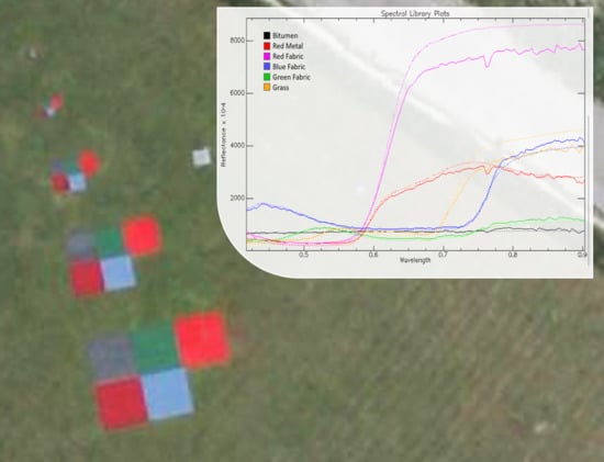
The experiments have been carried out on all datasets containing, as far as we have been able to verify, only six relevant materials as reported in Figure 5. These are the subsets Large Targets and All Targets Masked (containing pure and mixed pixels) and the subset Small Targets (containing only mixed pixels except for most grass image elements). The performance of each algorithm is evaluated by associating to each material in the HySpex spectral library (i.e., the solid lines in Figure 5) the extracted endmember yielding the minimum spectral angle [42]. Please note that a single extracted endmember could be the nearest neighbor to two different materials in the library: this does not bias the results of the analysis, as both spectral angles cannot be simultaneously small.

All algorithms with pure pixel assumptions were tested on the Large Targets dataset and their performance is reported in Figure 6a. Here, results from the best algorithm among the two based on minimum volume analysis, namely SISAL, are also reported. VCA and N-FINDR obtain the best results, with SISAL obtaining a poor performance, as does PPI with both the Python and MatLab implementations (both implementations give similar results, so we only report the former). For VCA and N-FINDR we have carried out a few trials to confirm that slight differences in the output would not affect the analysis, and show only a representative run. The results obtained by dictionary learning (DL), also shown in the plot, are competitive, but we defer their discussion to Section 6.1, while the performance of k-means is reported in Section 4.1. The locations of the retrieved endmembers are shown for the three best algorithms VCA, N-FINDR and ATGP in Figure 7. As hinted in Figure 6a, ATGP is missing the green fabric endmember and the largest distortion for bitumen is because the endmember chosen is a mixed pixel with the adjacent red metal sheets.

Results on the Small Targets subset are reported in Figure 6b. As expected, algorithms operating without the pure pixel assumption yield the best performance, with slightly better results obtained by SISAL. Improvements are however not substantial with respect to VCA and N-FINDR. All algorithms struggle at identifying the bitumen material, which is difficult to retrieve in a mixed setting due to the absence of clear absorption features in the analyzed spectral range. Furthermore, green fabric appears also here as a difficult material to find, probably due to some spectral features in common with the dominating grass spectra. Figure 8 shows the iterations of the SISAL algorithm, produced by its implementation in [22], showing the evolution of the endmembers in a squashed two-dimensional representation.

Results on the subset containing all targets with masked background are reported in Figure 9. If the ideal input number of endmembers $k=6$ is used as in Figure 9a, VCA obtains the best results, followed by N-FINDR and ATGP, which have problems with the bitumen and green fabric endmembers, respectively (see Figure 10). In Figure 9b we report results obtained by setting the input number of endmembers k as the value between 6 and 10 yielding the best results. In this case, additional endmembers which are not matched to any of the six spectra in the HySpex reference library in Figure 5 (solid lines) are simply ignored. Distortions are as expected reduced except for k-means (see dedicated Section 4.1), and VCA yields again the best performance, followed by N-FINDR. Again, the results of DL are discussed in Section 6.1. Despite the higher number of spectra extracted, ATGP does not manage to extract accurately the bitumen spectrum. This is shown also in Figure 11, reporting the locations of the extracted endmembers, where some additional materials detected by ATGP are still located in mixed image elements.

4.1. Clustering Experiment

To assess the separability of the different materials, we report an additional experiment involving k-means [41] in representation of clustering algorithms. To use k-means for endmembers extraction, we selected the cluster centroids output by the algorithm. K-means is not traditionally directly applied to this problem (with some exceptions, e.g., [43]): on the one hand, it does not locate pure pixels (the centroids usually do not exactly match any image element); on the other hand, it is not able to locate endmembers outside of the convex hull encompassing the data for a highly mixed scenario. Therefore, unsupervised clustering is rather used as a pre-processing step for other EE algorithms [44] and, to avoid confusion, k-means results are presented separately in this paragraph. We ran the algorithm using as input number of clusters $k=6$ on the Large Targets and All Targets Masked subsets. On the latter we also used $k=9$, as this yielded the best results in terms of spectral angle if k is allowed to vary between 6 and 10. Results reported in Figure 12 show a partial separation of the targets, with the bitumen and green fabric endmembers largely merged in a single cluster and the mixed pixels between red fabric and grass assigned to a separate cluster. As the number of clusters grow, larger number of mixed pixels form additional clusters. This explains the marginal improvement when increasing the value of k in Figure 9 in terms of spectral angle between cluster centroids and endmembers. Furthermore, it confirms that k-means is not reliable as a stand-alone endmember extraction method despite comparable results to traditional algorithms on the All Targets Masked subset.

5. Abundance Estimation

The last step in the spectral unmixing process is abundance estimation. This task consists of estimating the individual material abundances in each pixel given a library of spectral endmembers. As stated in Section 1, we adopt solely the linear mixture model (cf. Equation (1)). Please note that the abundances are not necessarily related to the relative areas occupied by the materials (for a discussion, see [1] and references therein). However, such assumption is made here along with linear mixing and the measured target areas are accordingly used as ground truth to evaluate the accuracy of abundance estimation. This simplified approach will be validated a posteriori by the obtained results. In the following we report on the application of widely used abundance estimation algorithms to the DLR HySU benchmark dataset. Unless otherwise stated, the reference spectral library extracted from the HySpex image (cf. solid lines in Figure 5) is used as input to the algorithms. This choice enables the evaluation of the abundance estimation process itself while being decoupled from any uncertainties introduced by endmember extraction. The robustness of our results against the choice of the spectral library is nevertheless investigated at the end of the section.

Four traditional algorithms commonly used for abundance estimation were evaluated: unconstrained least squares (UCLS), non-negative least squares (NNLS), fully constrained least squares (FCLS) [45] and least squares with least absolute shrinkage and selection operator (LASSO) [46]. All mentioned algorithms are based on least squares minimization, but the constraints applied on the abundances are distinct: UCLS finds the plain least squares solution without any constraints; NNLS and FCLS both require abundances to be non-negative (the so-called non-negativity constraint), with FCLS requiring in addition that the abundances sum to one (the so-called sum-to-one constraint); the version of LASSO used in this work implements the abundance non-negativity constraint and an upper limit $\lambda$ on the ${\ell }^1$-norm of the abundance vector, which induces sparsity. Although other methods exist in the literature, the mentioned algorithms, which also cover sparse analysis, are among the most relevant techniques in use within the hyperspectral community for linear unmixing. The results reported here are based on the MatLab implementation of UCLS, NNLS and FCLS [23] and on the Python implementation of LASSO in the SPAMS toolbox [47,48,49].

The abundance maps obtained with UCLS, NNLS, FCLS and LASSO (with $\lambda =1$) are shown in Figure 13. The six abundances (five materials plus vegetation background) for each algorithm are displayed in single RGB composites, where red metal and red fabric are associated with the red channel, green fabric and grass (the latter rescaled from 0 to 0.3 for visualization purposes) to the green channel, and blue fabric and bitumen to the blue channel. Since all tested algorithms perform unmixing for each pixel independently, the results in Figure 13 only had to be obtained once for the full subset. This is different from the case of the endmember extraction investigated in Section 4, where algorithms were tested in several subsets of the benchmark. Overall, the four unmixing techniques can derive abundance maps where most targets are well-defined with relatively crisp edges, little confusion between the materials and few false positives across the subset. It is clear that pure or close to pure pixels are identified in the 3 and 2m targets, while smaller targets correspond to highly mixed pixels as expected. The absence of visible aliasing effects in Figure 13 is due to a realistic abundance estimation of mixed pixels, yielding smooth transitions on boundaries between different materials. Figure 14 reports a detail of NNLS abundances for the largest targets, offering a more detailed overview about what happens in pixels with a high degree of mixture. The qualitative positive outcome of the abundance estimation step attests the accuracy of the unmixing algorithms as well as the quality of the reference spectral library. Two additional features in Figure 13 are worth pointing out. First, in all cases a large abundance of bitumen is found to the right of the 1m targets in the position of the SVC white panel (cf. position I in Figure 1a), as both bitumen and the white panel exhibit a similarly flat spectrum. Secondly, the vegetation background has been clearly singled out by unmixing with one endmember only despite the slight spectral variability of grass across the football field.

Moving to a quantitative analysis, the obtained abundances can be directly associated with the area of each target on the ground. The approximate areas of the deployed targets are 9, 4, 1, 0.25 and 0.0625 m${}^2$, corresponding approximately to 18.4, 8.2, 2.0, 0.5, and 0.1 pixels in the HySpex processed dataset of 0.7m spatial resolution, with the exact areas measured on site (cf. Appendix A) used for validation. The estimated area of a target t, denoted ${\widehat{A}}_t$, is derived from the abundance maps in Figure 13 as the integral of all fractional material abundances $\left\{x_i\right\}$ inside a region $R_t$ surrounding the target. This assumes implicitly the correspondence between abundances and fractional area occupied by the material inside the pixel. The region $R_t$ is defined by selecting the central pixel of each target and expanding the region until the abundance for the material of interest is $x<0.01$. The regions for the two smaller targets (0.25 and 0.5m) have been additionally dilated using as structuring element a disc with radius 1. The definition of $R_t$ was designed to ensure that all pixels containing the target signal (both pure and mixed) are included and simultaneously spurious abundances far from the target are neglected. The regions $R_t$ are depicted in Figure 15 with a brightness proportional to the number of different regions assigned to each pixel, and as a consequence to the potential degree of mixture. The estimated areas ${\widehat{A}}_t$ for all targets and unmixing algorithms are reported in

Table 2. Target areas derived from abundance estimation for the DLR HySU benchmark. The estimated areas are shown in black in units of pixels and can be compared to the actual measured areas in Table A2. For convenience, we report the signed relative error $({\hat{A}}_t-A_t)/A_t$ in parentheses and color code it to green when its absolute value is below 10%, orange between 10 and 25% and red above 25%. The unsigned relative error $|{\hat{A}}_t-A_t|/A_t$ is also recorded for each algorithm and target size averaged over the target materials.

Material	3m		2m		1m		0.5m		0.25m
UCLS
Bitumen	19.839	(+7.7%)	8.678	(+6.3)	3.221	(+60%)	0.555	(+5.5%)	0.363	(+185%)
Red metal	16.255	(−10%)	7.682	(−5.7%)	1.649	(−11%)	0.457	(−10%)	0.009	(>−93%)
Blue fabric	18.072	(−0.9%)	8.250	(−0.4%)	1.974	(−3.8%)	0.372	(−27%)	0.057	(>$-54\%$)
Red fabric	18.142	(−3.5%)	7.886	(−3.2%)	2.001	(−1.9%)	0.380	( −26%)	0.051	(−62%)
Green fabric	17.824	(−3.8%)	8.156	(−0.6%)	1.823	(−11%)	−0.164	(−133%)	−0.319	(#x2212;336%)
Average		5.2%		3.2%		18%		>40%		>146%
NNLS
Bitumen	18.356	(−0.4%)	8.000	(−2.0%)	2.534	(+26%)	0.416	(−21%)	0.166	(+30%)
Red metal	16.943	(−6.2%)	7.800	(−4.2%)	1.767	(−4.8%)	0.600	(+18%)	0.072	(−42%)
Blue fabric	18.175	(−0.4%)	8.401	(+1.4%)	2.065	(+0.7%)	0.474	(−7.0%)	0.124	(−1.2%)
Red fabric	17.603	(−6.4%)	7.833	(−3.8%)	1.907	(−6.6%)	0.418	(−19%)	0.142	(+7.3%)
Green fabric	17.616	(−4.9%)	7.739	(−5.7%)	1.832	(−10%)	0.239	(−53%)	0.175	(+29%)
Average		3.6%		3.4%		9.7%		23%		22%
FCLS
Bitumen	18.465	(+0.2%)	8.072	(−1.1%)	2.233	(+11%)	0.395	(−25%)	0.123	(−3.6%)
Red metal	17.157	(−5.0%)	7.825	(−3.9%)	1.766	(−4.9%)	0.627	(+23%)	0.141	(+15%)
Blue fabric	18.328	(+0.5%)	8.525	(+2.9%)	2.138	(+4.2%)	0.439	(−14%)	0.106	(−15%)
Red fabric	18.361	(−2.3%)	7.955	(−2.3%)	1.951	(−4.4%)	0.449	(−13%)	0.110	(−17%)
Green fabric	17.909	(−3.3%)	8.053	(−1.8%)	2.340	(+15%)	0.638	(+26%)	0.838	(+520%)
Average		2.3%		2.4%		7.9%		20%		>114%
LASSO (λ = 1)
Bitumen	18.311	(−0.6%)	8.011	(−)	2.519	(+25%)	0.416	(−21%)	0.166	(+30%)
Red metal	16.727	(−7.4%)	7.667	(−5.8%)	1.646	(−11%)	0.600	(+18%)	0.072	(−42%)
Blue fabric	18.417	(+0.9%)	8.595	(+3.7%)	2.183	(+6.4%)	0.474	(−7.0%)	0.124	(−1.2%)
Red fabric	18.440	(−1.9%)	8.009	(−1.6%)	1.983	(−2.8%)	0.482	(−6.4%)	0.142	(+7.3%)
Green fabric	17.283	(−6.7%)	7.436	(−9.4%)	1.663	(−19%)	0.239	(−53%)	0.175	(+29%)
Average		3.5%		4.5%		13%		21%		22%
N-FINDR+NNLS
Bitumen	16.383	(−11%)	7.391	(−9.5%)	2.809	(+40%)	0.571	(+8.6%)	0.378	(+196%)
Red metal	16.990	(−5.9%)	7.869	(−3.4%)	1.956	(+5.3%)	0.828	(+62%)	0.258	(+111%)
Blue fabric	18.211	(−0.2%>)	8.474	(+2.3%)	2.114	(+3.1%)	0.585	(+15%)	0.278	(+122%)
Red fabric	16.967	(−9.7%)	7.629	(−6.3%)	1.910	(−6.4%)	0.453	(−12%)	0.216	(+63%)
Green fabric	18.545	(+0.1%)	8.682	(+5.8%)	2.611	(+28%)	0.789	(+56%)	1.073	(+693%)
Average		5.4%		5.4%		16%		31%		237%

in units of pixels. Using the measured areas $A_t$ in

Table A2. Target areas in units of pixels. The areas in this table were derived from Table A1 using the approximate pixel area of ${0.7}^2$ m${}^2$ for the HySpex processed dataset.

Target Area [pix]	3 m	2 m	1 m	0.5 m	0.25 m
Bitumen	18.429	8.163	2.010	0.526	0.128
Red metal	18.061	8.143	1.857	0.510	0.123
Blue fabric	18.245	8.286	2.051	0.510	0.125
Red fabric	18.798	8.143	2.041	0.515	0.133
Green fabric	18.521	8.204	2.041	0.505	0.135

as ground truth, the unsigned relative error $|{\widehat{A}}_t-A_t|/A_t$ is plotted in Figure 16 for each target size, material and algorithm.

The area estimation results in Table 2 and Figure 16 reveal several interesting trends. It is remarkable that the areas of the targets on the ground can be reconstructed down to a few percent accuracy using hyperspectral data only, without obvious biases towards general over- or under-estimation of the areas. This lends credit to our initial assumption linking abundances to relative areas, and it constitutes a non-trivial, independent test of the linear mixing model. Overall, the linear model offers a good description of the DLR HySU benchmark. The area estimation accuracy is however not universally high and depends strongly on the unmixing algorithm of choice, target material and target size. These effects are now discussed in turn.

All four tested algorithms lead to similar area estimation results for the DLR HySU benchmark targets. However, the NNLS and LASSO ($\lambda =1$) algorithms give the most consistent estimates across the different target materials and sizes. The mean area estimation error for these algorithms ranges from ∼4% for the 3m targets up to ∼20% for the 0.25m targets. FCLS actually presents better mean accuracy for the 3, 2, 1 and 0.5m targets, but it evidently fails for the 0.25m green fabric target. The combination of the abundance non-negativity and abundance sum constraints in FCLS appears to be disadvantageous for unmixing small sub-pixel targets resembling the background vegetation. UCLS obtains results in line with the other algorithms for the larger targets, but it breaks down for the 0.5m green fabric target and all 0.25m targets. The lack of any abundance constraint seems to make UCLS particularly prone to noise, therefore delivering less meaningful abundances, in some cases negative (see green fabric targets of 0.5 and 0.25m in Table 2).

We have further tested the use of LASSO by trying different ${\ell }^1$-norm upper limits in the range $\lambda =0.8-10$. As illustrated in Figure 17, results are similar for $\lambda \ge 1$ and exactly the same for $\lambda \ge 1.2$, but degrade clearly for $\lambda <1$. This is likely a consequence of having a spectral library collected with endmembers from the hyperspectral image itself. For the corresponding pixels, the abundance vector is a single-entry vector with ${\parallel x\parallel }_1=1$, so any $\lambda <1$ will not allow such solution. We therefore show the main LASSO abundance estimation results for $\lambda =1$. It is interesting to notice that the results of NNLS and LASSO ($\lambda =1$) are identical for all 0.5 and 0.25m targets except the 0.5m red fabric target, cf. Table 2. This happens as NNLS and LASSO with $\lambda =1$ solve exactly the same least squares minimization problem when the optimal abundance vector is such that ${\parallel x\parallel }_1\le 1$. Both algorithms require abundance non-negativity and, in the case ${\parallel x\parallel }_1\le 1$, the LASSO upper limit ${\parallel x\parallel }_1\le \lambda$ with $\lambda =1$ becomes irrelevant, as illustrated in Figure 18. The right panel of the figure identifies the pixels for which NNLS found optimal abundance vectors with ${\parallel x\parallel }_1\le 1$, clearly confirming that for all 0.5 and 0.25m targets except the 0.5m red fabric target both algorithms are expected to provide the same exact solution. Naturally, the same statement applies to LASSO with $\lambda >1$.

Trends of the target area error according to material and size are shown in Figure 19a for LASSO ($\lambda =1$). Other unmixing algorithms are qualitatively similar as can be seen in Table 2, so we focus on LASSO results for discussion. The area of the blue and red fabric targets can be reconstructed with an error smaller than $2\%$ for the 3m targets and better than $10\%$ for all sizes. Overall, these are the targets for which the abundance estimation step works best. Bitumen target areas can also be reconstructed to within $2\%$ for the 3 and 2m targets, but the error rises to 20–30% for the smaller targets where mixed pixels are present. The low and flat reflectance spectrum of bitumen appears to be easily identifiable for pure or close to pure pixels, while being very difficult to single out in the case of highly mixed pixels. The worse results are obtained for red metal and green fabric, where the area error hover above $5\%$ for the 3 and 2m targets and reaches 40–50% for the smaller targets. As stated in Section 2, red metal and green fabric are indeed challenging materials: the former has a rugged surface and a tendency to produce specular reflections, while the later resembles the background vegetation. This might explain the worse results obtained for the two materials. Finally, we comment on the trend with target size. Apart from a handful of outliers, the general trend observed in Figure 19a shows that the area reconstruction error increases rapidly with decreasing target size. This is intuitively expected, because smaller targets are associated with mixed pixels, contributing to each spectrum a weaker signal which is closer in amplitude to the image noise. Geometrically speaking, the perimeter-to-area ratio of a square target increases as its side length decreases, and so does the area reconstruction relative error. In addition, it is expected that the contrast between the target material and the background vegetation plays a role, but the modeling of the reconstruction area error lies outside the scope of the present work.

Up to now the spectral library manually extracted from the HySpex image was used as input to the abundance estimation process. The robustness of the obtained results is now tested using instead a spectral library containing the mean SVC acquisitions on the ground, see dashed lines in Figure 5. Figure 19b shows the resulting target area errors for the case of LASSO ($\lambda =1$). The comparison of both panels in Figure 19 leads to interesting conclusions dependent on target material and size. For all target sizes, it is apparent that the results are fairly robust for red metal, red fabric and green fabric, but bitumen and blue fabric display some degree of sensitivity to the spectral library used. There is also a clear dependence on target size. The target area error for the larger targets (3 and 2m) for all materials degrades from <10% when using the HySpex spectral library to around $10\%$ when using the SVC library. The degradation is much more severe for the smallest 0.25m targets, while the results are comparable for the mid-size targets (0.5 and 1m). Overall, we conclude that the abundance estimation results for resolved targets are robust, which is consistent with the qualitative similarity of the two spectral libraries already apparent from Figure 5. Abundance estimation for sub-pixel targets is sensitive to the spectral library used and better results are obtained when the library is selected directly from the image.

6. Other Applications

The three critical steps of spectral unmixing (dimensionality estimation, endmember extraction and abundance estimation) have been scrutinized in the previous sections with the help of the DLR HySU benchmark. There are several other problems that can be investigated in detail with our benchmark dataset, some of which we address here in an illustrative preliminary fashion leaving an exhaustive study for future work. The community is invited to experiment with the DLR HySU benchmark for testing these and other applications.

6.1. Joint Endmember Extraction and Abundance Estimation

The endmember extraction and abundance estimation steps were tested separately in Section 4 and Section 5. A conceptually more difficult problem is that of jointly extracting endmembers and estimating abundances. Here we perform a limited set of experiments in this direction and show the typical accuracy attainable for endmember extraction and abundance estimation when carrying out both steps simultaneously. A thorough survey of state-of-the-art algorithms as done in Section 4 and Section 5 is outside the scope of the present work.

A simplified strategy to address the problem is to extract endmembers with one of the algorithms of Section 4 and then use these endmembers to estimate abundances with one of the algorithms of Section 5. Selecting within the best performing algorithms, the results of the combination of N-FINDR and NNLS are shown in Table 2 and Figure 16. N-FINDR+NNLS succeeds in recovering well the areas of the larger targets of red metal, blue fabric, red fabric and green fabric, but it has poor results for the smaller targets of those materials and for most targets of bitumen.

The previous approach, although straightforward, does not simultaneously solve endmember extraction and abundance estimation, a feature which other techniques available in the literature can achieve. Among them, dictionary learning decomposes the data as the product of a dictionary (i.e., a spectral library in our hyperspectral case) by a vector of coefficients (i.e., abundances), see e.g., [48]. For illustration purposes, the DL algorithm is implemented using the SPAMS toolbox [47,48,49] to derive endmembers and abundances for the DLR HySU benchmark. As with the LASSO settings, we enforce the abundance non-negativity constraint and set an upper limit $\lambda =1$ on the ${\ell }^1$-norm of the abundance vector. It is clear from Figure 6 and Figure 9 that DL endmember extraction is very competitive for the different subsets and even delivers some of the most accurate endmembers for all materials. In particular, DL achieves results comparable to VCA and N-FINDR for the Large Targets subset (Figure 6a) and the All Targets Masked subset (Figure 9). The DL results are excellent in terms of spectral angle, but it is important to note that our use of DL cannot fully recover the absolute spectra of Figure 5 as do the other endmember extraction algorithms of Section 4. This is because the SPAMS DL algorithm outputs ${\ell }^2$-normalized endmember spectra, therefore implying the loss of the ${\ell }^2$-norm of each spectrum. Notice that this is not necessarily a limitation of DL itself, but of the implementation used here. Despite the success of DL for endmember extraction, its performance is very poor on abundance estimation and is not shown in Table 2 or Figure 16. This is again due to the ${\ell }^2$-normalized extracted endmembers, which spoil the abundance estimation in mixed pixels.

Overall, both strategies studied briefly in this subsection (N-FINDR+NNLS and DL) offer in general a limited abundance estimation accuracy when compared to the best results of Section 5, where the reference spectral library was used as input. Notice however that a joint endmember extraction and abundance estimation might be the only option when no spectral library is available.

6.2. Hidden Target Detection

Along with the main targets used to investigate spectral unmixing, three small hidden targets were also included in the DLR HySU benchmark, namely a 0.25m square red metal target, a 0.5m square blue fabric target and a 0.5m square green fabric target. The three targets were placed across the test field over different backgrounds to test anomaly detection. The positions of the targets can be found in Figure 1a (F, G and H). The problem of hidden target detection can be formulated in different ways depending on whether the number, spectra and/or size of the targets is given as input. We suppose for concreteness that only the spectra of the targets to locate are given. In this case, spectral unmixing can be applied to estimate abundances and therefore pinpoint the desired material. For illustration, we show in Figure 20 the abundance maps of red metal, blue fabric and green fabric for the LASSO algorithm ($\lambda =1$) used in Section 5. It is clear from the figure that this straightforward approach is sufficient to locate the 0.5m blue and green fabric targets, but inadequate to identify the smaller 0.25m red metal piece. An added value of this approach is that it offers the possibility to estimate the target area. Other formulations of the hidden target detection and the study of dedicated anomaly detection algorithms are left for future research.

7. Conclusions

This paper introduces the DLR HySU (HyperSpectral Unmixing) benchmark dataset, consisting of a high-resolution airborne image acquired by the HySpex spectrometer in the VNIR range, completed by high-resolution airborne 3K RGB data, and in-situ SVC spectrometer measurements. The area of interest contains five synthetic targets of different materials in five different sizes, deployed on ground in a homogeneous area. The dataset allows testing all main steps of a typical spectral unmixing workflow, including dimensionality estimation, endmember extraction with and without pure pixel assumption, and abundance estimation. Further areas of research which can benefit from the DLR HySU dataset include target detection and denoising. Regarding the former, additional small targets have been scattered in the area of interest and are described in the paper. The latter can use the in-situ collected spectra as reference to verify denoising procedures on single targets, especially for bitumen which is characterized by a flat spectrum. Despite the relative simplicity of the targets arrangement, the described mixing scenarios result more accurate with respect to the ones currently available in the literature, as the surface area of all targets of different materials is known, and no additional materials are present in the scene, enabling a precise assessment of algorithm performance. Future datasets may include additional target materials and more complex mixing patterns in an effort to provide more realistic mixing scenarios.

Testing state-of-the art algorithms with the DLR HySU benchmark dataset for different steps of the unmixing procedure yielded several interesting results:

• The confirmation of overestimation by the most used dimensionality estimation method for imaging spectrometer data, HySime, in non-ideal settings, i.e., when applied to images too small in size with non-zero noise contribution.
• The comparison between algorithms working with or without the pure pixel assumption assessed on real data for different targets, suggesting that the latter family of algorithms may perform slightly better at handling complex, highly mixed data. To the best of our knowledge, this is the first time that a comparison between algorithms working with or without the pure pixel assumption is made on real data. In the past, such assessment was made on synthetic images [1].
• The equivalence between the NNLS and the LASSO methods for specific cases.
• The effects of enforcing the sum-to-one constraint in FCLS, often used in abundance estimation in the literature, which may introduce severe distortions in the case of image elements with a high degree of mixture. The last aspect adds up to the distortions introduced by FCLS whenever an incomplete spectral library is used [2].

With the experience gathered in previous campaigns and the one presented in this work, some aspects have been identified that should be taken care of when preparing a complex dataset of this kind. First, it would be desirable to have smaller GSD or larger targets deployed on ground to derive a spectral library from averaged spectra. As a rule of thumb, to ensure several pure pixels for all targets, the size of these should be set at least to five times the GSD. Secondly, the area containing the targets of interest should be as close as possible to sensor nadir to minimize spatial distortions due to aircraft roll movements. Furthermore, the integration time of the imaging spectrometer should be set to a low value if bright targets are chosen, as usually synthetic targets have a higher reflectance with respect to natural ones.

The DLR HySU benchmark dataset is open and available at [7]. The community is invited to make use of the dataset to test spectral unmixing and other applications, expanding the exploratory analysis we have presented in this work.

References

1. Bioucas-Dias, J.M.; Plaza, A.; Dobigeon, N.; Parente, M.; Du, Q.; Gader, P.; Chanussot, J. Hyperspectral Unmixing Overview: Geometrical, Statistical, and Sparse Regression-Based Approaches. IEEE J. Sel. Top. Appl. Earth Obs. Remote Sens. 2012, 5, 354–379. [Google Scholar] [CrossRef] [Green Version]
2. Cerra, D.; Müller, R.; Reinartz, P. Noise Reduction in Hyperspectral Images Through Spectral Unmixing. IEEE Geosci. Remote Sens. Lett. 2014, 11, 109–113. [Google Scholar] [CrossRef] [Green Version]
3. Altmann, Y.; Halimi, A.; Dobigeon, N.; Tourneret, J.Y. Supervised nonlinear spectral unmixing using a post-nonlinear mixing model for hyperspectral imagery. IEEE Trans. Geosci. Remote Sens. 2012, 21, 3017–3025. [Google Scholar]
4. Keshava, N.; Mustard, J.F. Spectral unmixing. IEEE Signal Process. Mag. 2002, 19, 44–57. [Google Scholar] [CrossRef]
5. Zhu, F. Hyperspectral unmixing: Ground truth labeling, datasets, benchmark performances and survey. arXiv 2017, arXiv:1708.05125. [Google Scholar]
6. Imbiriba, T.; Borsoi, R.; Bermudez, J. Low-Rank Tensor Modeling for Hyperspectral Unmixing Accounting for Spectral Variability. IEEE Trans. Geosci. Remote Sens. 2019, 58, 1833–1842. [Google Scholar] [CrossRef] [Green Version]
7. HySU Download Link. Available online: https://www.dlr.de/eoc/en/desktopdefault.aspx/tabid-12760/22294_read-73262/ (accessed on 7 June 2021).
8. Heylen, R.; Parente, M.; Gader, P. A Review of Nonlinear Hyperspectral Unmixing Methods. IEEE J. Sel. Top. Appl. Earth Obs. Remote Sens. 2014, 7, 1844–1868. [Google Scholar] [CrossRef]
9. Zhang, G.; Cerra, D.; Müller, R. Shadow Detection and Restoration for Hyperspectral Images Based on Nonlinear Spectral Unmixing. Remote Sens. 2020, 12, 3985. [Google Scholar] [CrossRef]
10. Dobigeon, N.; Altmann, Y.; Brun, N.; Moussaoui, S. Linear and Nonlinear Unmixing in Hyperspectral Imaging. In Resolving Spectral Mixtures with Applications from Ultrafast Time-Resolved Spectroscopy to Super-Resolution Imaging; Ruckebusch, C., Ed.; Data Handling in Science and Technology; Elsevier: Amsterdam, The Netherlands, 2016; Volume 30, pp. 185–224. [Google Scholar] [CrossRef]
11. Institute, D.R.S.T. Airborne Imaging Spectrometer HySpex. JLSRF 2016, 2, A93. [Google Scholar] [CrossRef] [Green Version]
12. Kurz, F.; Türmer, S.; Meynberg, O.; Rosenbaum, D.; Runge, H.; Reinartz, P.; Leitloff, J. Low-cost Systems for real-time Mapping Applications. Photogramm. Fernerkund. Geoinf. 2012, 159–176. [Google Scholar] [CrossRef]
13. Holben, B.; Eck, T.; Slutsker, I.; Tanré, D.; Buis, J.; Setzer, A.; Vermote, E.; Reagan, J.; Kaufman, Y.; Nakajima, T.; et al. AERONET—A Federated Instrument Network and Data Archive for Aerosol Characterization. Remote Sens. Environ. 1998, 66, 1–16. [Google Scholar] [CrossRef]
14. Krauß, T.; d’Angelo, P.; Schneider, M.; Gstaiger, V. The Fully Automatic Optical Processing System CATENA at DLR. ISPRS Int. Arch. Photogramm. Remote Sens. Spat. Inf. Sci. 2013, XL-1/W, 177–181. [Google Scholar] [CrossRef] [Green Version]
15. Baumgartner, A.; Köhler, C.H. Transformation of point spread functions on an individual pixel scale. Opt. Express 2020, 28, 38682–38697. [Google Scholar] [CrossRef] [PubMed]
16. Schwind, P.; Schneider, M.; Müller, R. Improving HySpex Sensor Co-Registration Accuracy using BRISK and Sensor-model based RANSAC. ISPRS Arch. 2014, XL-1, 371–376. [Google Scholar] [CrossRef] [Green Version]
17. Müller, R.; Lehner, M.; Müller, R.; Reinartz, P.; Schroeder, M.; Vollmer, B. A program for direct georeferencing of airborne and spaceborne line scanner images. Int. Arch. Photogramm. Remote Sens. Spat. Inf. Sci. 2002, 34, 148–153. [Google Scholar]
18. Richter, R.; Schläpfer, D. Geo-atmospheric processing of airborne imaging spectrometry data. Part 2: Atmospheric/topographic correction. Int. J. Remote Sens. 2002, 23, 2631–2649. [Google Scholar] [CrossRef]
19. Richter, R. Correction of satellite imagery over mountainous terrain. Appl. Opt. 1998, 37, 4004–4015. [Google Scholar] [CrossRef]
20. Bioucas-Dias, J.; Nascimento, J. Hyperspectral subspace identification. IEEE Trans. Geosci. Remote Sens. 2008, 46, 2435–2445. [Google Scholar] [CrossRef] [Green Version]
21. Wang, C.M.; Chen, C.; Chung, Y.N.; Yang, S.C.; Chung, P.C.; Yang, C.W.; Chang, C.I. Detection of spectral signatures in multispectral MR images for classification. IEEE Trans. Med. Imaging 2003, 22, 50–61. [Google Scholar] [CrossRef]
22. Bioucas Dias, J.M. Code, University of Lisbon. Available online: http://www.lx.it.pt/~bioucas/code.htm (accessed on 21 June 2021).
23. Gerg, I. Hyperspectral Toolbox. Available online: https://github.com/isaacgerg/matlabHyperspectralToolbox (accessed on 21 June 2021).
24. Chang, C. A Review of Virtual Dimensionality for Hyperspectral Imagery. IEEE J. Sel. Top. Appl. Earth Obs. Remote Sens. 2018, 11, 1285–1305. [Google Scholar] [CrossRef]
25. Prades, J.; Safont, G.; Salazar, A.; Vergara, L. Estimation of the Number of Endmembers in Hyperspectral Images Using Agglomerative Clustering. Remote Sens. 2020, 12, 3585. [Google Scholar] [CrossRef]
26. Drumetz, L.; Veganzones, M.A.; Marrero Gómez, R.; Tochon, G.; Mura, M.D.; Licciardi, G.A.; Jutten, C.; Chanussot, J. Hyperspectral Local Intrinsic Dimensionality. IEEE Trans. Geosci. Remote Sens. 2016, 54, 4063–4078. [Google Scholar] [CrossRef] [Green Version]
27. Ghamisi, P.; Yokoya, N.; Li, J.; Liao, W.; Liu, S.; Plaza, J.; Rasti, B.; Plaza, A. Advances in Hyperspectral Image and Signal Processing: A Comprehensive Overview of the State of the Art. IEEE Geosci. Remote Sens. Mag. 2017, 5, 37–78. [Google Scholar] [CrossRef] [Green Version]
28. Berman, M.; Hao, Z.; Stone, G.; Guo, Y. An Investigation Into the Impact of Band Error Variance Estimation on Intrinsic Dimension Estimation in Hyperspectral Images. IEEE J. Sel. Top. Appl. Earth Obs. Remote Sens. 2018, 11, 3279–3296. [Google Scholar] [CrossRef]
29. Plaza, J.; Hendrix, E.; García Fernandez, I.; Martín, G.; Plaza, A. On Endmember Identification in Hyperspectral Images Without Pure Pixels: A Comparison of Algorithms. J. Math. Imaging Vis. 2012, 42, 163–175. [Google Scholar] [CrossRef]
30. Alonso, K.; Bachmann, M.; Burch, K.; Carmona, E.; Cerra, D.; de los Reyes, R.; Dietrich, D.; Heiden, U.; Hölderlin, A.; Ickes, J.; et al. Data Products, Quality and Validation of the DLR Earth Sensing Imaging Spectrometer (DESIS). Sensors 2019, 19, 4471. [Google Scholar] [CrossRef] [Green Version]
31. Nascimento, J.M.P.; Dias, J.M.B. Vertex component analysis: A fast algorithm to unmix hyperspectral data. IEEE Trans. Geosci. Remote Sens. 2005, 43, 898–910. [Google Scholar] [CrossRef] [Green Version]
32. Winter, M.E. N-FINDR: An Algorithm for Fast Autonomous Spectral End-Member Determination in Hyperspectral Data. In Imaging Spectrometry V; Descour, M.R., Shen, S.S., Eds.; International Society for Optics and Photonics, SPIE: Washington, DC, USA, 1999; pp. 266–275. [Google Scholar] [CrossRef]
33. Ren, H.; Chang, C. Automatic spectral target recognition in hyperspectral imagery. IEEE Trans. Aerosp. Electron. Syst. 2003, 39, 1232–1249. [Google Scholar]
34. Chang, C.; Chen, S.; Li, H.; Chen, H.; Wen, C. Comparative Study and Analysis Among ATGP, VCA, and SGA for Finding Endmembers in Hyperspectral Imagery. IEEE J. Sel. Top. Appl. Earth Obs. Remote Sens. 2016, 9, 4280–4306. [Google Scholar] [CrossRef]
35. Therien, C. PySptools. Available online: https://pysptools.sourceforge.io/index.html (accessed on 21 June 2021).
36. Boardman, J.W. Geometric mixture analysis of imaging spectrometry data. In Proceedings of the IGARSS ’94-1994 IEEE International Geoscience and Remote Sensing Symposium, Pasadena, CA, USA, 8–12 August 1994; Volume 4, pp. 2369–2371. [Google Scholar] [CrossRef]
37. Bioucas-Dias, J.M. A variable splitting augmented Lagrangian approach to linear spectral unmixing. In Proceedings of the 2009 First Workshop on Hyperspectral Image and Signal Processing: Evolution in Remote Sensing, Grenoble, France, 26–28 August 2009. [Google Scholar] [CrossRef] [Green Version]
38. Miao, L.; Qi, H. Endmember Extraction From Highly Mixed Data Using Minimum Volume Constrained Nonnegative Matrix Factorization. IEEE Trans. Geosci. Remote Sens. 2007, 45, 765–777. [Google Scholar] [CrossRef]
39. Pedregosa, F.; Varoquaux, G.; Gramfort, A.; Michel, V.; Thirion, B.; Grisel, O.; Blondel, M.; Prettenhofer, P.; Weiss, R.; Dubourg, V.; et al. Scikit-learn: Machine Learning in Python. J. Mach. Learn. Res. 2011, 12, 2825–2830. [Google Scholar]
40. ITAKURA, F. Analysis synthesis telephony based on the maximum likelihood method. In Proceedings of the 6th International Congress on Acoustics, Tokyo, Japan, 21–28 August 1968. [Google Scholar]
41. MacQueen, J. Some methods for classification and analysis of multivariate observations. In Proceedings of the Fifth Berkeley Symposium on Mathematical Statistics and Probability, Oakland, CA, USA, 27 December 1965–7 January 1966; pp. 281–297. [Google Scholar]
42. Kruse, F.A.; Lefkoff, A.; Boardman, J.; Heidebrecht, K.; Shapiro, A.; Barloon, P.; Goetz, A. The spectral image processing system (SIPS)-interactive visualization and analysis of imaging spectrometer data. In AIP Conference Proceedings; American Institute of Physics: Pasadena, CA, USA, 1993; pp. 192–201. [Google Scholar]
43. Shah, D.; Zaveri, T.; Dixit, R. Hyperspectral Endmember Extraction Algorithm Using Convex Geometry and K-Means. In Emerging Technology Trends in Electronics, Communication and Networking; Gupta, S., Sarvaiya, J.N., Eds.; Springer: Singapore, 2020; pp. 189–200. [Google Scholar]
44. Martin, G.; Plaza, A. Region-Based Spatial Preprocessing for Endmember Extraction and Spectral Unmixing. IEEE Geosci. Remote Sens. Lett. 2011, 8, 745–749. [Google Scholar] [CrossRef] [Green Version]
45. Iordache, M.D.; Bioucas-Dias, J.; Plaza, A. Sparse Unmixing of Hyperspectral Data. IEEE Trans. Geosci. Remote Sens. 2011, 49, 2014–2039. [Google Scholar] [CrossRef] [Green Version]
46. Tibshirani, R. Regression Shrinkage and Selection via the Lasso. J. R. Stat. Society. Ser. B 1996, 58, 267–288. [Google Scholar] [CrossRef]
47. SPAMS (SPArse Modeling Software). Available online: http://spams-devel.gforge.inria.fr/index.html (accessed on 21 June 2021).
48. Mairal, J.; Bach, F.R.; Ponce, J.; Sapiro, G. Online Learning for Matrix Factorization and Sparse Coding. J. Mach. Learn. Res. 2010, 11, 19–60. [Google Scholar]
49. Mairal, J.; Bach, F.; Ponce, J.; Sapiro, G. Online Dictionary Learning for Sparse Coding. In Proceedings of the International Conference on Machine Learning, Montreal, QC, Canada, 14–18 June 2009. [Google Scholar]
Figure 1. DLR HySU benchmark targets. Panel (a) shows an RGB overview of the football field with the targets as imaged by the 3K camera. The ground track of the aircraft is shown by the dashed yellow line. The schematic configuration of the different targets is illustrated in (b) and a close-up of the target materials with the same spatial arrangement is shown in the bottom panel (c).
Remotesensing 13 02559 g001
Figure 2. Impressions from the field work during the DLR HySU benchmark campaign. The deployment of the large 3m targets and the small 0.25 and 0.5m targets is shown in (a,b), respectively. The typical measurement setup of the SVC field spectrometer can be seen in (c).
Remotesensing 13 02559 g002
Figure 3. Survey area located on DLR premises close to Munich, Germany. Relevant flight line and location of the deployed synthetic targets are overlaid.
Remotesensing 13 02559 g003
Figure 4. True color composites of the HySpex subsets provided in the DLR HySU benchmark dataset. The whole area of interest within a larger context is depicted in (a). All targets at different sizes and mixture levels are contained in subset (b). Here, the bright target in the upper part of the image to the right indicates the location of the white panel used as reference for the in-situ data collection. All area northeastern from the overlaid white line, also including mixtures of grass and road in the northeastern corner, can be masked out and excluded from endmember extraction assessments. A small subset with a high degree of mixture containing the small 0.25 and 0.5m targets only is reported in (c). The case of the large 3 m targets only is represented in (d). Here, the locations of image elements collected for the spectral library reported in Figure 5 are marked in white. A full description of each subset in given in Section 2.2.2.
Remotesensing 13 02559 g004
Figure 5. Spectral library manually extracted from the HySpex image (solid lines) compared to mean SVC acquisitions (dashed lines). The HySpex spectra are selected in the center of the corresponding 3 m targets (marked in white in Figure 4d), while the grass spectrum represents the dominant background. The individual SVC acquisitions leading to the mean SVC measurement shown here can be found in Figure A1. Wavelengths are expressed in micrometers.
Remotesensing 13 02559 g005
Figure 6. Spectral angle between endmembers extracted by different EE algorithms and the HySpex reference spectra reported in Figure 5. The algorithms have been applied to the subset containing the large 3 m targets only (a), which should be the easier case, and on the scenario containing no pure endmembers (b), which is a highly mixed scenario. VCA and N-FINDR algorithms retrieve the correct spectra with the least amount of distortion for the large targets (see also Figure 7), while the SISAL [37] and NMF algorithms operating without the pure pixel assumption obtain slightly better results in the mixed scenario. The results of dictionary learning (DL) will be discussed in Section 6.1.
Remotesensing 13 02559 g006
Figure 7. Locations of endmembers extracted from algorithms working under the pure pixel assumption on the Large Targets subset using as input number of endmembers k = 6 .
Remotesensing 13 02559 g007
Figure 8. SISAL iterations shown in a two-dimensional projection of the spectral parameter space for the Small Targets subset. The blue dots represent the data points and the red ones the endmembers identified in consecutive iterations up to convergence to the chosen solution shown as green dots.
Remotesensing 13 02559 g008
Figure 9. Spectral angle between endmembers extracted by different EE algorithms and the HySpex reference spectra reported in Figure 5. In (a), the input number of endmembers k = 6 has been used, while in (b) the best k between 6 and 10 was chosen according to the best results (k indicated in parenthesis for each method).
Remotesensing 13 02559 g009
Figure 10. Locations of endmembers extracted from algorithms working under the pure pixel assumption on the subset All Targets Masked using as input number of endmembers k = 6 .
Remotesensing 13 02559 g010
Figure 11. Locations of endmembers extracted from algorithms working under the pure pixel assumption on the subset All Targets Masked using as input number of endmembers k the best value between 6 and 10, indicated in brackets for each algorithm.
Remotesensing 13 02559 g011
Figure 12. K-means clustering on subsets Large Targets and All Targets Masked. The number of endmembers k used in each case is shown in brackets. The centroids of each cluster are matched to the endmembers in the HySpex reference spectral library in Figure 5.
Remotesensing 13 02559 g012
Figure 13. Abundance maps obtained by spectral unmixing for the DLR HySU benchmark. The results for UCLS, NNLS, FCLS and LASSO ( λ = 1 ) are combined in a single RGB representation. The abundances (stretched from 0 to 1) are color-coded as follows: red metal and red fabric in red, green fabric and grass in green, bitumen and blue fabric in blue. The grass abundance was rescaled from 0 to 0.3 in order not to hide the boundary with green fabric.
Remotesensing 13 02559 g013
Figure 14. Detail of Figure 13b for abundances computed with the NNLS algorithm on the 3 and 2 m targets, with grid showing single image elements overlaid.
Remotesensing 13 02559 g014
Figure 15. Regions R t where abundances contribute to the estimation of the area for each target t. Brightest pixels indicate that an image element is considered for several targets, i.e., it may have a higher degree of mixture. Pixels where contributions from a single material are expected are represented in dark red, while pixels where five materials can contribute, as in the smallest targets to the north, are depicted in white.
Remotesensing 13 02559 g015
Figure 16. Target area error from abundance estimation for the DLR HySU benchmark. The unsigned relative error | A ^ t A t | / A t displayed here for each algorithm, target size and target material was obtained by combining the estimated areas from Table 2 and the actual measured areas from Table A2.
Remotesensing 13 02559 g016
Figure 17. Effect of 1 -norm upper limit λ on LASSO area estimation results. The unsigned relative error | A ^ t A t | / A t is shown averaged over target materials and separately for the different target sizes.
Remotesensing 13 02559 g017
Figure 18. Equivalence of NNLS and LASSO ( λ = 1 ) abundance estimation framework. The left panel (a) illustrates a toy example for NNLS and LASSO ( λ = 1 ) solutions in an abundance space spanned by two endmembers only. The UCLS solution and corresponding square error contours are shown in blue, while the abundance vector found by NNLS and LASSO is marked with a red cross. In both cases the NNLS and LASSO find the same solution since the LASSO constraint x 1 λ = 1 is satisfied. The right panel (b) indicates the pixels in the DLR HySU benchmark with an abundance vector found by NNLS with x 1 1 in dark blue (yellow in the area surrounding the targets) and with x 1 > 1 in light blue (red in the area surrounding the targets). Yellow pixels highlight target pixels with x 1 1 , for which NNLS and LASSO ( λ = 1 ) are equivalent. Except for the 0.5m red fabric target, all pixels corresponding to the 0.5 and 0.25m targets are yellow in the right panel (b), therefore explaining the exact same estimated areas for these targets with NNLS and LASSO ( λ = 1 ) in Table 2.
Remotesensing 13 02559 g018
Figure 19. Target area error for different target materials and sizes for LASSO ( λ = 1 ). The error measure shown here is the unsigned relative error | A ^ t A t | / A t . The results are shown for the case of using the spectral library collected from the HySpex image (a) and from the mean SVC acquisitions (b).
Remotesensing 13 02559 g019
Figure 20. Hidden target detection through spectral unmixing. The RGB composite shows the LASSO ( λ = 1 ) abundance maps for red metal (red), green fabric (green) and blue fabric (blue), clipped and displayed in logarithmic scale to facilitate the identification of hot spots. The red boxes are centered at the positions of the hidden targets (F, G, H) as inferred from the 3K image. The 0.5m hidden targets made of blue fabric (G) and green fabric (H) are fairly visible, while the 0.25m red metal piece (F) cannot be located. The SVC white panel (I) can be clearly seen in the blue fabric abundance map.
Remotesensing 13 02559 g020