Article

Machine Learning Techniques to Predict Soybean Plant Density Using UAV and Satellite-Based Remote Sensing

by
Luthfan Nur Habibi
1,
Tomoya Watanabe
2,
Tsutomu Matsui
3 and
Takashi S. T. Tanaka
3,4,*
1
Graduate School of Natural Science and Technology, Gifu University, Gifu 5011193, Japan
2
Graduate School of Mathematics, Kyushu University, Fukuoka 8190395, Japan
3
Faculty of Applied Biological Sciences, Gifu University, Gifu 5011193, Japan
4
Artificial Intelligence Advanced Research Center, Gifu University, Gifu 5011193, Japan
*
Author to whom correspondence should be addressed.
Remote Sens. 2021, 13(13), 2548; https://doi.org/10.3390/rs13132548
Submission received: 30 May 2021 / Revised: 27 June 2021 / Accepted: 28 June 2021 / Published: 29 June 2021
(This article belongs to the Special Issue UAV Imagery for Precision Agriculture)

Abstract

:
The plant density of soybean is a critical factor affecting plant canopy structure and yield. Predicting the spatial variability of plant density would be valuable for improving agronomic practices. The objective of this study was to develop a model for plant density measurement using several data sets with different spatial resolutions, including unmanned aerial vehicle (UAV) imagery, PlanetScope satellite imagery, and climate data. The model establishment process includes (1) performing the high-throughput measurement of actual plant density from UAV imagery with the You Only Look Once version 3 (YOLOv3) object detection algorithm, which was further treated as a response variable of the estimation models in the next step, and (2) developing regression models to estimate plant density in the extended areas using various combinations of predictors derived from PlanetScope imagery and climate data. Our results showed that the YOLOv3 model can accurately measure actual soybean plant density from UAV imagery data with a root mean square error (RMSE) value of 0.96 plants m−2. Furthermore, the two regression models, partial least squares and random forest (RF), successfully expanded the plant density prediction areas with RMSE values ranging from 1.78 to 3.67 plant m−2. Model improvement was conducted using the variable importance feature in RF, which improved prediction accuracy with an RMSE value of 1.72 plant m−2. These results demonstrated that the established model had an acceptable prediction accuracy for estimating plant density. Although the model could not often evaluate the within-field spatial variability of soybean plant density, the predicted values were sufficient for informing the field-specific status.

Graphical Abstract

1. Introduction

In soybean (Glycine max (L.) Merr.) production, ensuring a high plant density is one of the main ways to maximize crop yield [1,2,3]. Plant density is a product of seedling rates and stands establishment ratios. However, soybean establishment is highly variable depending on climate and soil conditions [4,5]. Furthermore, there is an optimal plant density for maximizing yield according to the environment [6] and genotype [7], because an excessively high soybean population affects plant structure, mainly by reducing the number of pods per plant. Thus, the quantification of plant density is an essential step to identifying the optimal plant population, row spacing, and seed density during sowing, which could contribute to developing better crop management practices. Given the recent diffusion of precision agricultural technologies, such as variable-rate seeding, not only field-specific but also within-field variability of plant density should be quantified.
Evaluating plant density can be done by manually counting the soybean stands in the field by employing various methods, such as systematic design counting, which can assess a wide range of soybean plant densities [8]. However, this kind of method is labor-intensive and time-consuming. Although the optimal seeding rates have been tested in field-scale trials [9,10], information on final plant density is mostly unavailable. Detailed spatial information on plant density, which cannot be assessed by manual measurement, is needed to provide better prescriptions across fields. Thus, it is essential to develop a high-throughput measurement method for plant density.
The application of remote sensing technology has been widely addressed in agricultural fields using various platforms, such as satellite, aircraft, and unmanned aerial vehicles (UAVs), to achieve better efficiency, cost-effectiveness, and high-throughput measurement, rather than direct monitoring on the field [11]. The determination of suitable remote sensing instruments for measuring a specific variable is crucial to obtaining the appropriate method and data set [12], since each platform has different specifications, namely, the spatial and temporal resolution, flight altitude, acquisition schedule, spectral ranges, operational cost, and others [13]. The measurement of plant density requires explicit information on the individual plant canopies in high accuracy of the quantification and geographic location in a detailed scale. The remote sensing scene can be used to access individual plant stands with a canopy delineation process to obtain the location, size, shape, and number of plant canopies [14]. In larger vegetation canopies, such as forest vegetation, satellite remote sensing has been widely used to delineate vegetation canopy at the tree-crown scale [15,16]. However, commonly used optical satellite imagery, such as Landsat (30 m resolution), Sentinel-2 (10 m resolution), and PlanetScope (3 m resolution), has an insufficient spatial resolution to detect small canopy, namely, crop plants [15]. Crop plant density that represents the geometrical agronomic trait [11,17] is more challenging to be measured using satellite imagery, since the majority of satellite imagery does not provide a detailed spatial resolution that can show textures or geometrical features of crop plants; thus, it prevents directly accessing the number of plants inside the pixels. Crop plant density usually has a dense population in a one-meter square area that is hard to capture using either satellite- or aircraft-based remote sensing. The limitation of the spatial resolution of satellite-based remote sensing instruments prevents high-throughput analysis for small grain crops.
Each remote-sensing instrument and platform has different characteristics such as spatiotemporal resolution, coverage, and spectral specifications. Thus, a multiscale remote sensing and image analysis has been applied to compensate for each other’s shortcomings. For instance, a synergy between satellite imagery and finer resolution imagery captured by other platforms that can precisely observe an object can expand the observation coverage on a global scale to break the resolution limitation in satellite imagery [18]. This approach has been widely applied in forestry studies for measuring plant populations by using airborne-based light detection and ranging (LiDAR) and satellite imagery together [14,19]. Data accessed from LiDAR can assess the individual structure of plants, such as height and canopy area, then incorporated with satellite imagery data (e.g., spectral reflectance) to measure plant populations in a broader coverage using regression analysis [19]. A similar approach should be applied in agricultural studies for accessing crop growth status, which is plant density; however, to the best of our knowledge, this kind of approach has not yet been applied for soybean production. The utilization of LiDAR was also used to quantify small grain crop plant density with great accuracy, as proposed by Saeys et al. [20]; however, it has a significant shortcoming, since the sensor must be mounted on a combine harvester, causing limited area observation. Moreover, the cost of LiDAR sensors is not affordable for most farmers. As a substitute to LiDAR, UAV imagery can record photogrammetry scenes, presenting geometric agricultural traits on a detailed scale.
Unmanned aerial vehicles have been widely used in scientific research for several years with the benefits of flexible time and flight operation and cloud-free data [21]. Unmanned aerial vehicles are commonly equipped with high-resolution camera sensors that are capable of providing high spatial resolution, depending on the platform’s height. Photogrammetry can also provide geometrical traits of vegetation similar to LiDAR. The use of UAVs in the study of delineating or detecting a single crop plant also became a trend in the last decade with the rise of machine learning techniques. Object detection algorithms have become a popular approach to identifying an individual crop canopy from photogrammetry images. The combination of UAV imagery and machine learning has been applied to accurately estimate the numbers of plants of various crops, including soybean [22], rice [23], wheat [24], maize [25], rapeseed [26], and cotton [27], and is even used to detect weed seedlings in cultivation fields [28]. The proposed methods in the literature have utilized machine learning techniques that provide high accuracy output for detecting individual plants in UAV imagery; thus, the quantification of field plant density can be accurately measured. However, since previous studies only utilized a single remote sensing instrument—namely, UAV—with the flight altitude limited to a maximum height of 20 m to keep the high spatial resolution imagery, the area coverage became limited to a few hectares in a single flight. Considering that farmers have broad fields, monitoring plant density with UAV will be a challenging task.
As noted above, satellite imagery is directly incapable of identifying individual plants because of the limited resolution; however, optical sensors of satellite imagery can provide surface reflectance values and vegetation indices, reflecting the plant biomass and leaf area index [29]. Plant biomass per unit area is a product of individual plant biomass and plant density. Therefore, surface reflectance values and vegetation indices are hypothesized to be indirect predictors for estimating plant density by referring to the values at the same phenological stage as long as the individual plant biomass is almost constant. Thus, accurately measured plant population from UAV imagery by the object detection algorithm are expected to be a response variable for plant density estimation model, which treats reflectance data and vegetation indices derived from satellite imagery as predictors in a wider area coverage of observations. In addition to remote sensing data, climate data, such as precipitation and air temperature, might be important elements in predicting the plant density, since it could affect seedling establishment and plant growth such as leaf area expansion [5,30,31].
The aim of this study was to develop a satellite-based model for estimating soybean plant density through machine learning techniques. Specifically, the high-throughput measurement of actual plant density quantified by UAV imagery and YOLOv3 models was used as the response variable for plant density estimation models, while PlanetScope imagery and climate data were used as predictors for the models. The prediction accuracies of partial least squares (PLS) regression and random forest (RF) regression were compared in developing estimation models, as these methods were reported to be robust for dealing with remote sensing imagery data [32,33,34,35,36,37]. Finally, the spatial pattern of plant density was further assessed using the developed model to examine the potential implications for better crop management practices and the limitations of the satellite-based models.

2. Materials and Methods

In order to establish models to predict the plant density of soybean, we divided the workflow of the study into three steps: (1) performing high-throughput measurement of actual plant density of the observation fields from UAV imagery using an object detection model based on the You Only Look Once version 3 (YOLOv3) algorithm, which was further treated as a response variable in the regression model development; (2) performing preprocessing of the PlanetScope imagery to fill in the gaps of missing daily spectral reflectance data using spline smoothing, which served as predictor variables from satellite imagery data; (3) establishing satellite-based plant density estimation models using two regression analysis methods, PLS and RF regression, to expand the measurement of plant density into wider area coverage. The flow chart in Figure 1 summarizes all of the steps involved in this study.

2.1. Study Area

This study was conducted in 12 soybean fields in Kaizu City, Gifu, Japan. The soybean fields were planted between the 2018 and 2020 growing seasons from July–November for each year. The farmers in this location implemented crop rotation with three crops (paddy rice–winter wheat–soybean) over two years, which became a challenging task to find exactly the same fields cultivating soybean in multiple years sequentially. Thus, fields in different locations for each year were observed for the analysis. A local leading soybean cultivar, ‘Fukuyutaka’, was grown in all observation fields. According to a previous study [38], the optimum planting date of the ‘Fukuyutaka’ cultivar was approximately 10 July. However, the sowing dates of the observed fields were varied due to the climate conditions, as machinery cannot be used for seeding several days after heavy rain. The differences in sowing dates and soil conditions during the seeding caused unstable seedling establishment rate and plant density variability in fields. Thus, selected fields sown from the optimum to late sowing dates in the three years were surveyed to cover high variations of plant density. The detailed locations map and sowing dates for the research fields are presented in Figure 2 and Table 1.

2.2. Imagery and Climate Data Collection

2.2.1. Acquisition of UAV Imagery

A total of 12 soybean field scenes were taken under natural daylight conditions. All imagery was captured during the early stage of soybean growth (emergence stage) from 11 days after sowing (DAS) until 22 DAS (Table 1). The image data sets were captured using a commercial UAV (Phantom 4 Pro, DJI, Shenzhen, China) equipped with a default RGB camera capturing 5472 × 3648 pixel images for each scene. The number of scenes was different for each field depending on the area coverage. Images were captured from 15 m above the surface, resulting in a ground sampling distance of approximately 3.5 mm per pixel. The trajectory of the UAV was set to ensure a 60–70% front and side image overlap. The coordinates of ground control points (GCPs) for registering the camera location were measured using KlauPPK (Klau Geomatics, New South Wales, Australia) with 0.03 m precision. Using this georeferencing process, we could minimalize the geographical error regarding the location of each soybean stand measured in the following procedure (Section 2.3). The orthomosaic for each field was generated using Structure from Motion (SfM) software (Pix4D, Pix4Dmapper version 4.6.4, Lausanne, Switzerland). The average pixel size per field of the orthomosaics was 61,036 × 28,113 pixels.

2.2.2. PlanetScope Imagery Data

This study used the PlanetScope surface reflectance product taken with PS2 and PS2.SD instruments (Planet Labs Inc., San Francisco, CA, USA). This product provides ground sample distance at 3 m per pixel, captured using a four-band frame imager including blue (PS2: 455–515 nm; PS2.SD: 464–517 nm), green (PS2: 500–590 nm; PS2.SD: 547–585 nm), red (PS2: 590–670 nm; PS2.SD: 650–682 nm), and near-infrared (NIR) (PS2: 780–860 nm; PS2.SD: 846–888 nm). The imagery was already orthorectified and geometrically corrected using altitude telemetry and ephemeris data with refined GCPs by the provider to deal with geographical errors [39]. Moreover, all available imagery was already atmospherically corrected by Planet Labs Inc. before they released it in their application programming interface framework. This correction was crucial for the study, since we used spectral reflectance values of the imagery. The PlanetScope satellite constellation is capable of recording the land surface at a daily frequency. In this study, we used PlanetScope scenes of the observation fields from the sowing dates until 60 DAS. However, the terrestrial surface was sometimes covered with thick clouds, which made daily observations difficult. Thus, we tried to download the available cloudless imagery that clearly shows the fields and processed the imagery in the following procedure (Section 2.4) to acquire a daily spectral reflectance value. The imagery was very limited in 2020 because of frequent bad weather during the growing season. The number of PlanetScope scenes used for each field is listed in Table 1.

2.2.3. Climate Data

Daily total rainfall (mm) and mean air temperature (°C) were obtained from the Agro-Meteorological Grid Square Data, NARO [40] (https://amu.rd.naro.go.jp/, accessed on 23 October 2020). Daily data were downloaded for the months of the soybean growing season (July–October) in 2018–2020. The meteorological data had an approximately 1 km2 resolution based on the reference mesh area used by the data provider. Ideally, higher-resolution data for the climate would have been utilized to match the resolution of the satellite imagery and to understand the spatial variations more precisely. However, such data were not available without in situ measurement; thus, we used these data as a substitute for the meteorological data.

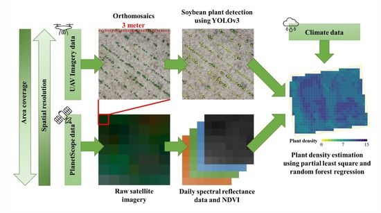
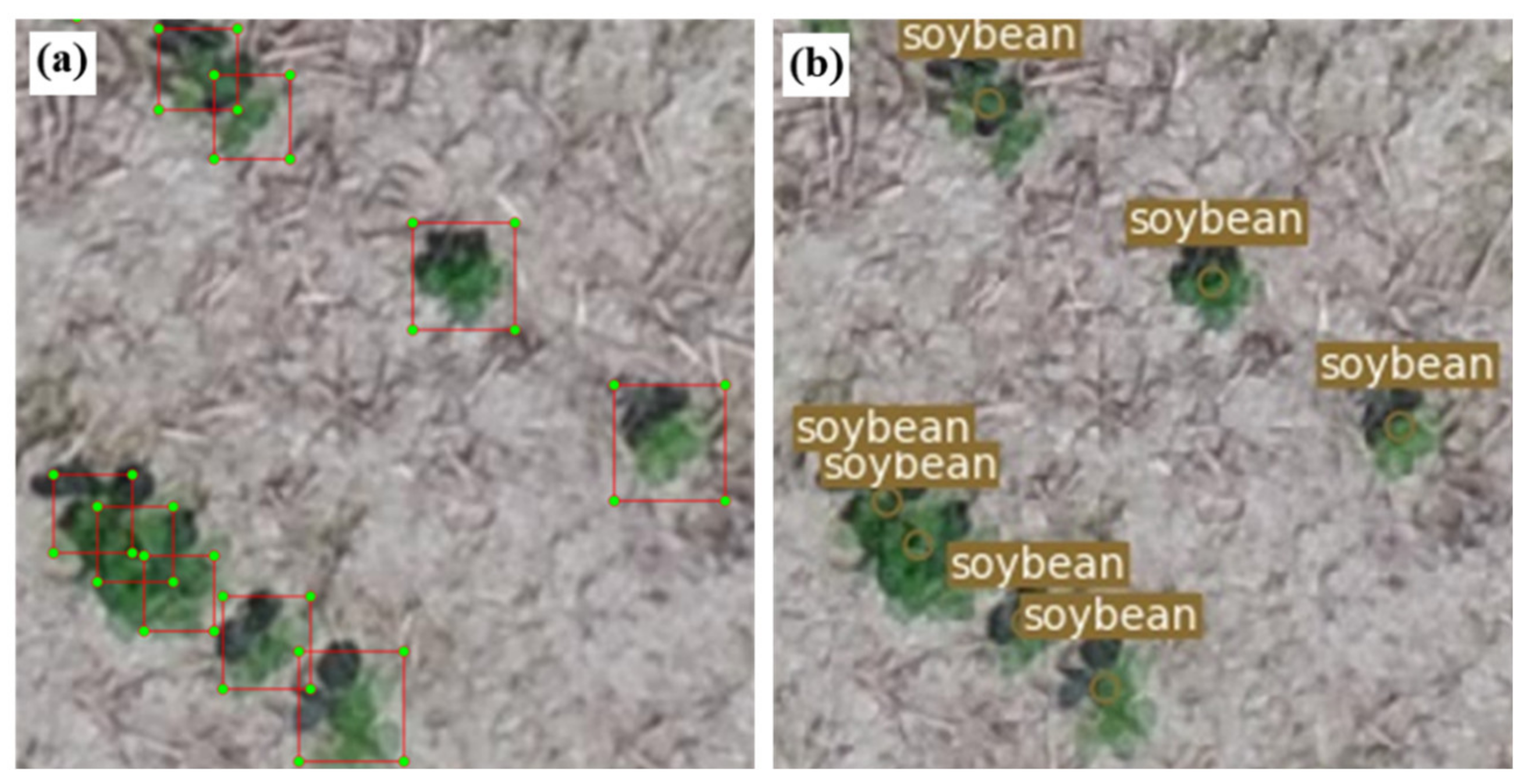
2.3. Actual Plant Density Measurement from UAV Imagery Using YOLOv3

Firstly, the number of soybean plants were accurately measured to obtain the actual plant density data of the observation fields. This data will be used as the response variable for the plant density estimation model using satellite imagery and climate data. The high-throughput detection of soybean plants was carried out using the YOLOv3 algorithm that is capable of extracting the number and exact location of the plant canopies from UAV imagery; thus, actual plant density can be evaluated by calculating the number of plants divided by the area.
YOLOv3 is an end-to-end object detection algorithm based on a deep learning neural network [41]. The YOLOv3 network contained 53 convolutional layers, known as Darknet-53, with improved detection speed and accuracy, and was designed to be more suitable for small object detection than the previous generation [41,42]. This feature makes YOLOv3 a suitable algorithm for detecting individual soybean plants from UAV imagery.
The input dimensions for the YOLOv3 network were 416 × 416 × 3. To meet the input dimension, the orthomosaics were split into 416 × 416 pixel images using the virtual raster function in QGIS software (QGIS Development Team 2001, version 3.14), which resulted in a total of 129,520 images. From the split images, 712 images were randomly selected for YOLOv3 model establishment. The training, validation, and test data sets contained 278 (40%), 186 (25%), and 248 (35%) images, respectively. Each soybean plant in the split images was annotated with a bounding box using LabelImg [43], as shown in Figure 3a. To establish the best YOLOv3 model for counting the number of established soybean plants, a confidence threshold affecting object detection accuracy was tested from 0.05 to 0.95 at intervals of 0.05. The epoch size for the training processes was constant at 50. The batch size was set at 4 to speed up the training process due to the limited workstation specs (Intel Core i7-7820X, Nvidia GeForce GTX 1070, 72 GB of RAM and a Windows 10 Pro 64-bit system operation). The prediction accuracy was evaluated based on the coefficient of determination (r2), and root mean square error (RMSE) values obtained from calculations between the manually and automatically counted established soybean plants from the test data set by the developed models using a different confidence threshold value. The best model was determined by the highest r2 and lowest RMSE values.
The final process of YOLOv3 was to conduct soybean plant detection from all available split images. The Geospatial Data Abstraction Library (GDAL) function was used in this process to extract the centroid coordinates of the bounding boxes of detected soybean plants according to the world files that contained coordinates for each split image. The detected soybean plants with coordinate data were used for further regression analysis as described in Section 2.5.

2.4. Daily Spectral Reflectance Gap-Filling of PlanetScope

PlanetScope imagery data were used in this study to expand the high-throughput measurement of plant density in a wider coverage based on the actual plant density obtained from the YOLOv3 model (Section 2.3). PlanetScope imagery had a daily temporal resolution that was robust for identifying plant phenology, as we tried to measure the plant density in the later growth stages of soybean. However, due to the frequent observations using many satellites with various illumination geometries and poor inter-sensor calibration, the temporal surface reflectance data of PlanetScope became less stable and noisy [29]. Figure 4 shows that the raw spectral reflectance data of PlanetScope (presented as points) were not stable throughout the growth durations. Moreover, surface reflectance derived from satellite imagery were inherently noisy due to the variable illumination patterns and aerosols in the atmosphere. Smoothing splines can be used to reduce the potential for noise from the spectrum wavelength [44].
The process was started by extracting the spectral reflectance values of every pixel within the observation field areas using the zonal statistic function in QGIS software. The available raw spectral reflectance data of PlanetScope imagery were then processed using the spline function implemented in the ‘stats’ package in R (R Development Core Team 2019, version 3.5.3). As presented in Figure 4, the distribution of available spectral reflectance data was scattered between the sowing date and 60 DAS. A smoothing spline can also be used to interpolate spectral reflectance values of the missing date due to the presence of thick clouds from the available data. On the other hand, the smoothness of the spline curves can be set to make flexible curves by increasing the degree of polynomial or the number of knots. However, increasing the number of knots can lead to overfitting, while a small number of knots may result in restricted data that have more bias. Therefore, four knots were used in the smoothing spline process to obtain the natural shape of the curve. Our data set had a small range of examples, so a higher number of knots would overfit the data.
Furthermore, we also calculated the daily normalized difference vegetation index (NDVI) value [45] from the interpolated spectral reflectance of PlanetScope imagery, because it represents the most commonly used vegetation indices that are capable of assessing a particular variable of vegetation, e.g., quantity, quality, and vegetation stage developments [19]. The normalized difference vegetation index was calculated using PlanetScope bands with the equation: (NIR − Red)/(NIR + Red). Data for the interpolated spectral reflectance and NDVI value from this process were used as predictor variables in the regression analysis (Section 2.6).

2.5. Selecting Variables

Three data sources with different spatial resolutions (UAV imagery with 0.03 × 0.03 m2, PlanetScope imagery with 3 × 3 m2, and climate data with 1 × 1 km2) were used to develop the plant density prediction model. Regression analysis using statistical and machine learning methods was used for the model. The selection of variables, both for response and predictors, is crucial in regression analysis. The response variable for the regression model was the soybean plant density derived from the number of plants counted by the YOLOv3 best model (Section 2.3). For the predictors, PlanetScope imagery data (spectral reflectance and NDVI) and climate data (precipitation and temperature) were selected. The first predictor, the spectral reflectance values of all PlanetScope bands, was used from every pixel in the observation field to examine the potential of each band in explaining plant density. Second, NDVI values calculated from the spectral reflectance value of PlanetScope imagery was used in the regression analysis. Moreover, we also minded the temporal resolution of the satellite imagery for increasing the capability of regression models in estimating plant density. Spectral reflectance and NDVI data were selected every ten days, calculated from the sowing dates (10, 20, 30, and 40 DAS) to reflect the growing process of the plants, as time series data could be valuable information for detecting plant density in the later growth stages. The last predictor variables were derived from climate data with the following details: (1) seven-day precipitations before and after the sowing date calculated from daily values; (2) ten-day cumulative temperatures at 10, 20, 30, and 40 DAS, calculated from the daily mean air temperature. All data from YOLOv3 model, PlanetScope imagery, and climate data were transformed into averaged values within each 3 × 3 m2 grid cell to match pixels area of PlanetScope. Details about the predictor variables are summarized in Table 2. The data were divided into training and test data sets by randomly selecting the observation fields. In this process, we also considered the potential effect of different years on plant density, as the climate condition varied largely from year to year; thus, the training and test datasets were not divided by the years. Training data were obtained using PlanetScope pixels in Fields 1, 4, 5, 6, 7, 10, and 12 (n = 6600), while pixels in the other five fields were used as test data (n = 5839).

2.6. PLS and RF Regression

In this study, two regression models, including PLS and RF regression, were used to establish the model for estimating plant density. These two methods are based on different analyses, where the PLS is a representative of the statistical approach, while RF is a representative of the machine learning technique. The main reason for using PLS and RF regression is because these approaches can deal with highly intercorrelated data such as the spectral reflectance data of satellite imagery. Conventional regression analysis, such as multiple linear regression, cannot handle multi-temporal satellite imagery data due to the fact of multi-collinearity problems [46].
Partial least squares regression is a generalized multiple linear regression that provides a multivariate approach to predicting one response variable using strongly collinear (correlated) predictor variables [47,48]. Details of PLS regression can be found in Geladi et al. [49]. A partial least squares regression model was established using the ‘pls’ package implemented in R [50]. In the analysis of PLS regression, the number of components was determined using the ‘selectNcomp’ function attached to the ‘pls’ package, according to the one-sigma method. The one-sigma heuristic chooses the fewest components for the model that has an accuracy of less than one standard error from the best model.
Random forest regression is one of the techniques in machine learning that can be used to estimate the response variable, based on classification and regression tree (CART) [51]. This analysis is efficient in processing non-linear data, which can also be found in the data set [32]. Details about RF can be found in Breiman [51]. A random forest regression model was established using the ‘randomForest’ package [52] implemented in R. Two parameters were adjusted to optimize the RF regression model: ntree, the number of trees grown in the regression forest, was set at 100; mtry, the number of different predictors sampled at each node (default = the number of predictors divided by 3).
The selection of predictors is an important process for the model’s establishment, as it could greatly affect the prediction accuracy and facilitate a better understanding of the relationships between predictors and response variables [12]. Thus, the PLS and RF regression models were trained to estimate plant density using several possible predictor variable combinations, as follows: (1) using spectral reflectance values only; (2) using NDVI values only; (3) using a combination of spectral reflectance and NDVI; (4) using a combination of PlanetScope imagery and climate data. The variable combinations were used to test the impact of different predictors in estimating plant density.
In addition, we also examined the variable importance measurement from RF regression as a method to determine the suitable variable predictors for predicting soybean plant density. This method has been widely used in many scientific fields to select and identify relevant predictors for predicting response variables [53]. Variable importance can be extracted from the regression trees by calculating IncNodePurity, which is the total decrease in node impurities from the splitting on the predictors, using the importance function in the ‘randomForest’ package. An increase in the value of IncNodePurity implies a decrease in the mean square error, which means that the largest values represent the most important variables to the response [54]. Variable importance was evaluated from the RF model with all available predictor variables. We verified whether the variable predictors with high values of IncNodePurity could improve the prediction capability of the developed regression model, since the predictors with low IncNodePurity are less critical to the response variable. The performance of all developed regression models in this section was compared based on r2 and RMSE values to see the best-fitted model, which were further used for spatial prediction of soybean plant density for the test fields.

3. Results

3.1. UAV Imagery and YOLOv3 Model Accuracy

We trained the YOLOv3 object detection model for high-throughput measurement of soybean plant numbers from the UAV imagery data. The effect of various confidence thresholds on the accuracy of the YOLOv3 model was examined to establish the most accurate model detecting the soybean seedling in the test data set images. The established YOLOv3 model with a 0.50 confidence threshold scored the highest accuracy with an r2 value of 0.88 and RMSE of 0.96 plants m−2 as shown in Figure 5. The results from the other models with different confidence threshold values are listed in Table S1. The YOLOv3, as the best model using the confidence threshold of 0.50, was hereafter applied for the UAV imagery of all observation fields to measure the actual plant density value, which was further used as the response variable of the PLS and RF regression models.

3.2. Accuracy of PLS and RF Regression Model

We created six models using different predictor variable combinations for the regression analysis using PLS and RF regression. The names and details of the models are listed in Table 3. In general, the RF regression outperformed the PLS regression in all combinations of predictors for both the training and test data sets (Table 3). The results showed that the high accuracy in the training data set did not always represent high accuracy in the test data set. In the test data, the PLS regression models scored an RMSE between 2.08 and 3.67 plants m−2 (r2 = 0.19–0.56), while the RF regression models scored between 1.78 and 1.92 plants m−2 (r2 = 0.60–0.67).
The partial least squares regression models with different variable combinations showed different results in estimating plant density as presented in Figure 6. The partial least squares regression model using variables SR + NDVI (SR + NDVI-PLS) gave the highest accuracy to estimate the test dataset (r2 0.56 and RMSE 2.08 plants m−2). Partial least squares regression using the SR-only predictor (SR-only PLS) performed similar results to SR + NDVI-PLS, with higher plant density variation, ranging from –0.95 to 12.41 plants m−2. In contrast, PLS regression using the NDVI-only predictor (NDVI-only PLS) scored the lowest variance, ranging from 1.04 to 8.04 plants m−2.
The results of the RF regression models using different variable combinations presented in Figure 7. The RF model using NDVI and climate data as variable predictors (NDVI + Climate-RF) that scored the highest accuracy was NDVI + Climate-RF (r2 0.67 and RMSE 1.78 plants m−2). The model with the lowest accuracy was the RF model using NVDI only predictors (NDVI-only RF). The accuracy of RF models was surpassed the PLS models in estimating plant density in test fields.
In addition to the RF analysis, we examined the variable importance of the RF model using all available predictors, and the results are shown in Figure 8. The results revealed that NIR at 40 DAS was the most influential variable for the model with more than 12,000 values of IncNodePurity, followed by precipitation before the sowing date, temperature at 10 DAS, and NIR at 30 DAS. The NDVI variables in the later DAS (40, 20, and 30 DAS) dominated the top ten variables. The temperature variables had little impact on the model accuracy, excluding that on DAS 10. The result indicated that most of the predictors were less important for the model to estimate the response variable, since the IncNodePurity was less than 20% of the highest variable, NIR at 40 DAS.
Based on the variable importance of the RF model using all available predictors, we developed another model using the top ten variables with the highest IncNodePurity score (10VarImp-RF). The newly developed RF regression model, 10VarImp-RF, scored the best performance (r2 0.68 and RMSE 1.72 plants m−2), as presented in Figure 9, which outperformed the best RF regression model without variable selection, according to the variable importance (NDVI + Climate-RF) and the best PLS regression model (SR + NDVI-PLS) in the test dataset, as presented in Table 3, Figure 6c and Figure 7e. The plant density estimated by the 10VarImp-RF model ranged from 0.40 to 11.70 plants m−2.

3.3. Spatial Prediction

The plant density spatial distribution maps of the test fields were created based on four methods: the YOLOv3 best model; SR + NDVI-PLS; NDVI + Climate-RF; 10VarImp-RF model (Figure 10). The YOLOv3 distribution map reflects the actual plant density of the fields, as it was measured by counting the accurate plant numbers inside the UAV imagery. Visually, the YOLOv3 model demonstrated the spatial variability of plant density in the test fields with a relatively wide variation in the within-field patterns, especially in Fields 2 and 8. From this distribution map, it was also possible to highlight field-specific plant density. Overall, the distribution maps based on the listed regression models could reflect the general pattern of the plant density spatial variability for both within-field and field-specific patterns. The distribution maps derived from NDVI + Climate-RF and 10VarImp-RF showed almost similar results, with minor differences in a few locations due to the higher sensitivity for small plant density in the 10VarImp-RF map, as shown in Fields 2 and 4 (Figure 10).
For further analysis of the comparison between actual and estimated spatial distribution maps, residual maps were created (Figure 11). In general, the residual maps resemble the spatial distribution of the actual plant density derived from the YOLOv3 model (Figure 10a), with some highlighted features on the overestimated and underestimated pattern from the estimated plant density values. According to the residual map (Figure 11), the spatial patterns showed similar tendencies, although there were differences in degrees across the field. In Field 3, all regression models showed underestimated patterns across the fields. On the other hand, in Field 9, almost two-thirds of the area of the field had a tendency of overestimation, while small areas in the southeast of the field had a tendency to underestimate. In Field 8, the most contrasting differences between the PLS model and RF models was that the underestimation pattern was obvious in SR + NDVI-PLS model. The field-specific RMSE values showed that the accuracy of the models was different from field to field, as the RMSE values ranged between 1.38 and 3.06 plant m−2 (Table 4).

4. Discussion

4.1. Quality of Measured Actual Plant Density Using YOLOv3 Model

In the YOLOv3 model process, confidence threshold values were tuned to construct the most accurate model. The developed YOLOv3 model in this study was capable of measuring soybean plant density accurately, as the RMSE was less than 1.0 plants m−2 (Figure 5). This result is in agreement with a previous study that quantified cotton plant density using UAV imagery and a YOLOv3 model with an RMSE between 0.50 and 1.14 plants m−2 [17]. Given that the detected plant density varied from 0 to 16.11 plants m−2 (Table S2), the detection accuracy of the model was considered to be adequate for representing the actual plant density spatial variance at the emergence in fields (Figure 10).

4.2. Factors Affecting the Accuracy of the Regression Models

Our results indicate that soybean plant density can be estimated using PlanetScope imagery and climate data with acceptable accuracy. Overall, RF regression models outperformed PLS regression models (Table 3). Random forest has been reported as a superior regression model to PLS regression [32,35,36], which is consistent with our results. As indicated by the r2 and RMSE values in the RF models, the NDVI + Climate-RF and SR + NDVI were likely to have the best performance. The model performance significantly decreased when predicting the test data set as compared to training data set (Table 3). Data distribution differences between each observation field used in the training and test data set might have caused the different output accuracy of the models. In our data sets, each field had a unique data distribution, from low to high values of plant density, and the majority of the field had a low variance. Thus, data variance between the training and test fields might have become unbalanced. The details about descriptive statistics for each observation field is presented in Table S2. Completely random data split might be a solution to improve model performance. However, completely random data split might not be the appropriate way in our case, because we must examine not only the overall prediction accuracy but also the effect of observation year and within-field prediction accuracy.
The different predictor combinations in the regression model development affected the accuracy of the estimation. The NDVI data used in the regression models might lead to underestimated plant densities in high population values. Previous studies [55,56] reported that there were underestimated trends in estimating biomass using NDVI but only seen in high values of biomass. The NDVI had limitations in losing the sensitivity of the plant canopy when the leaf area index was greater than 3 m2 m−2 [57], which corresponds to a high plant density. According to Mutanga and Skidmore [58], this phenomenon is called NDVI saturation, which subsequently contributed to a reduced accuracy in estimating plant-related variables. Concerning another predictor, climate variables also contributed to the inconsistent output of the regression model, especially in PLS analysis (Figure 6d–f). This inconsistency might be due to the other environmental or edaphic factors that we did not consider in our models, even though the same pattern did not appear on the RF models, possibly due to the better capability of non-linear relationships.

4.3. Benefit of Variable Importance of Random Forest

In this study, the variable importance in RF analysis was used to determine important predictor variables for developing a better estimation model and for improving prediction accuracy. This method has been used to determine the important variable of RF regression in predicting plant density and vegetation biomass using vegetation indices and multispectral instruments [22,59,60]. The newly developed model based on this method, the 10VarImp-RF model, showed a better prediction value (r2 0.68 and RMSE 1.72 plants m−2) than the other regression models (Figure 9). The accuracy of the 10VarImp-RF model was more robust compared to a previous study by Randelović et al. [22], who also predicted soybean plant density using RF regression treating multiple vegetation indices derived from an RGB UAV imagery as explanatory variables (RMSE: 3.91–7.47 plants m−2). Thus, the 10VarImp-RF model result may indicate that the selection of predictor variables based on variable importance would be an effective approach. Although the variable selection was reported to generate some bias in the classification task of RF, the potential of causing biased results in regression tasks has not been discussed [61]. The results demonstrated that variable selection might also be an essential process in enhancing the prediction accuracy of the RF model for regression tasks.
The variable importance of the RF regression model indicated that the NIR bands at 30 and 40 DAS were the first and fifth most important variables, respectively (Figure 8). Near-infrared reflectance is sensitive to changes in vegetation structure and leaf area index [29], which was also influential in predicting plant density. The normalized difference vegetation index at 20, 30, and 40 DAS was also within the ten most important variables. Overall, PlanetScope reflectance and NDVI values from the later growth stage that were close to flowering time, which was approximately 30–40 DAS, played relatively important roles in predicting plant density compared to the early growing stage. Red, green, and blue bands did not appear in the fifth most important variables.
The variable importance of RF regression further indicated that precipitation before sowing dates affected the plant density of soybean, probably because water availability is the main factor affecting the vegetation growth of plants [30]. Rainfall events could provide favorable conditions for both seedling emergence and subsequent leaf expansion. On the other hand, excessive soil moisture and submergence due to the heavy rain is reported to result in low emergence rate of seedling [5] and to retard leaf expansion in the early vegetative stage [31]. Therefore, rainfall data may have nonlinear effects on either leaf area or plant density. The significant errors in the PLS regression models for Field 9 (Figure 6d–f) also indicate the importance of nonlinear relationships between precipitation and plant density, because PLS regression is theoretically based on a linear assumption between the variables. Furthermore, a suitable temperature in the early days of emergence is also needed for seedlings to the emergence and represents the importance of cumulative temperature at 10 DAS in the RF model. High temperatures and low precipitation rates after sowing could promote drought, which could also decrease or delay emergence and plant growth [62]. The soybean growth rate in the juvenile stage after emergence responds strongly to temperature and water stress conditions [63]. Thus, climate data might have contributed to increasing the RF model’s accuracy (Table 3). However, note that climate data had a 1 km2 spatial resolution, resulting in almost regionally identical values across fields; thus, it could not contribute to increasing the prediction accuracy in terms of within-field spatial variability of plant density. To improve the model’s capability in the future, we should further consider including field microclimate data, including soil moisture content and temperature, by using an in situ measurement apparatus or synthetic-aperture radar.

4.4. Plant Density Distribution Map and Future Development

The plant density distribution map can provide a better understanding of identifying areas with low or high plant density dependencies for better management practices. The distribution map derived from the YOLOv3 model (Figure 10a) clearly shows the within-field and between-field patterns of plant density spatial variability. However, the distribution maps derived from regression models could not always clearly evaluate the within-field spatial variability of soybean plant density, although they might provide good information for identifying field-specific patterns. The spatial trends in prediction residuals (Figure 11) were not entirely at random, because each model shows similar tendencies in the same places across the fields. Other factors, namely, edaphic factors might have contributed to the spatial patterns, since it could affect within-field variability in individual aboveground biomass, leaf area index, and canopy structure, thus decreasing the prediction accuracy derived from the regression models. To improve the within-field spatial prediction accuracy, the edaphic factors affecting plant density should be quantified and included as predictors. As noted above, the effect of field microclimate data on the prediction accuracy should also be quantified in further study.

5. Conclusions

This study demonstrates that the satellite-based RF regression model successfully identified field-specific plant density. First, UAV imagery data processed using the YOLOv3 object detection model can be used to accurately measure the soybean plant density with an RMSE value of 0.96 plants m−2. The area coverage for the measurement of plant density was extended by utilizing PlanetScope imagery and climate data, which have a wider range than UAV imagery. The regression analysis using PLS and RF was capable of predicting the plant density of test fields with RMSE values ranging from 1.78 to 3.67 plant m−2. The selection of predictor variables based on the variable importance feature in RF analysis significantly improved the prediction accuracy with an RMSE value of 1.72 plant m−2 (10VarImp-RF model). The satellite-based prediction model might be able to provide farmers with useful information about field-specific variability in plant density. However, there might be a room to improve the prediction accuracy for explaining within-field variability in plant density because the plant density was likely to be influenced by edaphic factors that could not be quantified in this study. To the best of our knowledge, this is the first case study establishing satellite-based estimation model for soybean plant density. The proposed method in this study is expected to be adapted for other locations and different crops by arranging a suitable training process. Further research is needed to examine the potential uses of predicted plant density maps by analyzing the effects of edaphic factors and agronomic practices.

Supplementary Materials

The following are available online at https://www.mdpi.com/article/10.3390/rs13132548/s1, Table S1: Comparison of the output accuracy of the YOLOv3 models with different confidence threshold values, Table S2: Descriptive statistics of the actual plant density data derived from YOLOv3 model for the observation fields, Table S3: Descriptive statistics of the estimated plant density data derived from three regression models (SR + NDVI-PLS, NDVI + Climate-RF, 10VarImp-RF) for the test fields.

Author Contributions

Conceptualization, L.N.H., T.M. and T.S.T.T.; methodology, L.N.H., T.W. and T.S.T.T.; software, L.N.H., T.W. and T.S.T.T.; validation, L.N.H. and T.S.T.T.; formal analysis, L.N.H.; investigation, L.N.H. and T.S.T.T.; resources, T.M. and T.S.T.T.; data curation, L.N.H. and T.S.T.T.; writing—original draft preparation, L.N.H.; writing—review and editing, T.M. and T.S.T.T.; visualization, L.N.H.; supervision, T.M. and T.S.T.T.; project administration, T.S.T.T.; funding acquisition, T.S.T.T. All authors have read and agreed to the published version of the manuscript.

Funding

This research was funded by JSPS (Japan Society for the Promotion of Science) KAKENHI Early-Career Scientists Grant 18K14452, The OGAWA Science and Technology Foundation Research Grant, and MAFF (Ministry of Agriculture, Forestry and Fisheries, Japan) Commissioned Project Study JP J008719.

Institutional Review Board Statement

Not applicable.

Informed Consent Statement

Not applicable.

Data Availability Statement

The data presented in this study are available within the manuscript and in the Supplementary Materials.

Acknowledgments

The authors wish to thank the farming companies ‘Fukue-eino’ and ‘Kamigiri-eino’ for allowing the survey of their fields. The first author also acknowledges the Ministry of Education, Culture, Sports, Science, and Technology (MEXT) for providing master’s student scholarship under the Japanese Government MEXT scholarship program.

Conflicts of Interest

The authors declare no conflict of interest.

References

  1. Ball, R.A.; Purcell, L.C.; Vories, E.D. Optimizing Soybean Plant Population for a Short-Season Production System in the Southern USA. Crop Sci. 2000, 40, 757–764. [Google Scholar] [CrossRef]
  2. Gan, Y.; Stulen, I.; van Keulen, H.; Kuiper, P.J. Physiological response of soybean genotypes to plant density. Field Crops Res. 2002, 74, 231–241. [Google Scholar] [CrossRef]
  3. De Bruin, J.L.; Pedersen, P. New and Old Soybean Cultivar Responses to Plant Density and Intercepted Light. Crop Sci. 2009, 49, 2225–2232. [Google Scholar] [CrossRef]
  4. Lamichhane, J.R.; Constantin, J.; Schoving, C.; Maury, P.; Debaeke, P.; Aubertot, J.-N.; Dürr, C. Analysis of soybean germination, emergence, and prediction of a possible northward establishment of the crop under climate change. Eur. J. Agron. 2020, 113, 125972. [Google Scholar] [CrossRef]
  5. Takeda, H.; Sasaki, R. Effects of Ground Water Level Control on the Establishment, Growth and Yield of Soybeans Seeded during and after the Rainy Season. Jpn. J. Crop Sci. 2013, 82, 233–241, (In Japanese with English Summary). [Google Scholar] [CrossRef] [Green Version]
  6. Carciochi, W.D.; Schwalbert, R.; Andrade, F.H.; Corassa, G.M.; Carter, P.; Gaspar, A.P.; Schmidt, J.; Ciampitti, I.A. Soybean Seed Yield Response to Plant Density by Yield Environment in North America. Agron. J. 2019, 111, 1923–1932. [Google Scholar] [CrossRef] [Green Version]
  7. Rigsby, B.; Board, J.E. Identification of soybean cultivars that yield well at low plant populations. Crop Sci. 2003, 43, 234–239. [Google Scholar] [CrossRef]
  8. Egli, D.B. Plant Density and Soybean Yield. Crop Sci. 1988, 28, 977–981. [Google Scholar] [CrossRef]
  9. Corassa, G.M.; Amado, T.J.C.; Strieder, M.L.; Schwalbert, R.; Pires, J.L.F.; Carter, P.R.; Ciampitti, I.A. Optimum soybean seeding rates by yield environment in southern Brazil. Agron. J. 2018, 110, 2430–2438. [Google Scholar] [CrossRef]
  10. Gaspar, A.P.; Mourtzinis, S.; Kyle, D.; Galdi, E.; Lindsey, L.E.; Hamman, W.P.; Matcham, E.G.; Kandel, H.J.; Schmitz, P.; Stanley, J.D.; et al. Defining optimal soybean seeding rates and associated risk across North America. Agron. J. 2020, 112, 2103–2114. [Google Scholar] [CrossRef] [Green Version]
  11. Weiss, M.; Jacob, F.; Duveiller, G. Remote sensing for agricultural applications: A meta-review. Remote Sens. Environ. 2020, 236, 111402. [Google Scholar] [CrossRef]
  12. Hunt, M.L.; Blackburn, G.A.; Carrasco, L.; Redhead, J.W.; Rowland, C.S. High resolution wheat yield mapping using Sentinel-2. Remote Sens. Environ. 2019, 233, 111410. [Google Scholar] [CrossRef]
  13. Matese, A.; Toscano, P.; Di Gennaro, S.F.; Genesio, L.; Vaccari, F.P.; Primicerio, J.; Belli, C.; Zaldei, A.; Bianconi, R.; Gioli, B. Intercomparison of UAV, aircraft and satellite remote sensing platforms for precision viticulture. Remote Sens. 2015, 7, 2971–2990. [Google Scholar] [CrossRef] [Green Version]
  14. Dalponte, M.; Frizzera, L.; Gianelle, D. Individual tree crown delineation and tree species classification with hyperspectral and LiDAR data. PeerJ 2019, 2019. [Google Scholar] [CrossRef]
  15. Wang, J.; Yang, D.; Detto, M.; Nelson, B.W.; Chen, M.; Guan, K.; Wu, S.; Yan, Z.; Wu, J. Multi-scale integration of satellite remote sensing improves characterization of dry-season green-up in an Amazon tropical evergreen forest. Remote Sens. Environ. 2020, 246, 111865. [Google Scholar] [CrossRef]
  16. Wu, S.; Wang, J.; Yan, Z.; Song, G.; Chen, Y.; Ma, Q.; Deng, M.; Wu, Y.; Zhao, Y.; Guo, Z.; et al. Monitoring tree-crown scale autumn leaf phenology in a temperate forest with an integration of PlanetScope and drone remote sensing observations. ISPRS J. Photogramm. Remote Sens. 2021, 171, 36–48. [Google Scholar] [CrossRef]
  17. Oh, S.; Chang, A.; Ashapure, A.; Jung, J.; Dube, N.; Maeda, M.; Gonzalez, D.; Landivar, J. Plant counting of cotton from UAS imagery using deep learning-based object detection framework. Remote Sens. 2020, 12, 2981. [Google Scholar] [CrossRef]
  18. Emilien, A.-V.; Thomas, C.; Thomas, H. UAV & satellite synergies for optical remote sensing applications: A literature review. Sci. Remote Sens. 2021, 3, 100019. [Google Scholar] [CrossRef]
  19. Blázquez-Casado, Á.; Calama, R.; Valbuena, M.; Vergarechea, M.; Rodríguez, F. Combining low-density LiDAR and satellite images to discriminate species in mixed Mediterranean forest. Ann. For. Sci. 2019, 76. [Google Scholar] [CrossRef]
  20. Saeys, W.; Lenaerts, B.; Craessaerts, G.; De Baerdemaeker, J. Estimation of the crop density of small grains using LiDAR sensors. Biosyst. Eng. 2009, 102, 22–30. [Google Scholar] [CrossRef]
  21. Floreano, D.; Wood, R.J. Science, technology and the future of small autonomous drones. Nature 2015, 521, 460–466. [Google Scholar] [CrossRef] [Green Version]
  22. Ranđelović, P.; Đorđević, V.; Milić, S.; Balešević-Tubić, S.; Petrović, K.; Miladinović, J.; Đukić, V. Prediction of Soybean Plant Density Using a Machine Learning Model and Vegetation Indices Extracted from RGB Images Taken with a UAV. Agronomy 2020, 10, 1108. [Google Scholar] [CrossRef]
  23. Wu, J.; Yang, G.; Yang, X.; Xu, B.; Han, L.; Zhu, Y. Automatic Counting of in situ Rice Seedlings from UAV Images Based on a Deep Fully Convolutional Neural Network. Remote Sens. 2019, 11, 691. [Google Scholar] [CrossRef] [Green Version]
  24. Jin, X.; Liu, S.; Baret, F.; Hemerlé, M.; Comar, A. Estimates of plant density of wheat crops at emergence from very low altitude UAV imagery. Remote Sens. Environ. 2017, 198, 105–114. [Google Scholar] [CrossRef] [Green Version]
  25. Zan, X.; Zhang, X.; Xing, Z.; Liu, W.; Zhang, X.; Su, W.; Liu, Z.; Zhao, Y.; Li, S. Automatic Detection of Maize Tassels from UAV Images by Combining Random Forest Classifier and VGG16. Remote Sens. 2020, 12, 3049. [Google Scholar] [CrossRef]
  26. Zhang, J.; Zhao, B.; Yang, C.; Shi, Y.; Liao, Q.; Zhou, G.; Wang, C.; Xie, T.; Jiang, Z.; Zhang, D.; et al. Rapeseed Stand Count Estimation at Leaf Development Stages with UAV Imagery and Convolutional Neural Networks. Front. Plant Sci. 2020, 11, 617. [Google Scholar] [CrossRef] [PubMed]
  27. Jiang, Y.; Li, C.; Paterson, A.H.; Robertson, J.S. DeepSeedling: Deep convolutional network and Kalman filter for plant seedling detection and counting in the field. Plant Methods 2019, 15, 141. [Google Scholar] [CrossRef] [PubMed] [Green Version]
  28. Peña, J.M.; Torres-Sánchez, J.; Serrano-Pérez, A.; de Castro, A.I.; López-Granados, F. Quantifying efficacy and limits of unmanned aerial vehicle (UAV) technology for weed seedling detection as affected by sensor resolution. Sensors 2015, 15, 5609–5626. [Google Scholar] [CrossRef] [PubMed] [Green Version]
  29. Cheng, Y.; Vrieling, A.; Fava, F.; Meroni, M.; Marshall, M.; Gachoki, S. Phenology of short vegetation cycles in a Kenyan rangeland from PlanetScope and Sentinel-2. Remote Sens. Environ. 2020, 248, 112004. [Google Scholar] [CrossRef]
  30. Khaliliaqdam, N.; Soltani, A.; Latifi, N.; Ghaderi Far, F. Soybean Seed Aging and Environmental Factors on Seedling Growth. Commun. Soil Sci. Plant Anal. 2013, 44, 1786–1799. [Google Scholar] [CrossRef]
  31. Bajgain, R.; Kawasaki, Y.; Akamatsu, Y.; Tanaka, Y.; Kawamura, H.; Katsura, K.; Shiraiwa, T. Biomass production and yield of soybean grown under converted paddy fields with excess water during the early growth stage. Field Crops Res. 2015, 180, 221–227. [Google Scholar] [CrossRef]
  32. Liu, J.; Sun, S.; Tan, Z.; Liu, Y. Nondestructive detection of sunset yellow in cream based on near-infrared spectroscopy and interval random forest. Spectrochim. Acta Part A Mol. Biomol. Spectrosc. 2020, 242, 118718. [Google Scholar] [CrossRef] [PubMed]
  33. Inoue, Y.; Sakaiya, E.; Zhu, Y.; Takahashi, W. Diagnostic mapping of canopy nitrogen content in rice based on hyperspectral measurements. Remote Sens. Environ. 2012, 126, 210–221. [Google Scholar] [CrossRef]
  34. Vaglio Laurin, G.; Chen, Q.; Lindsell, J.A.; Coomes, D.A.; Del Frate, F.; Guerriero, L.; Pirotti, F.; Valentini, R. Above ground biomass estimation in an African tropical forest with lidar and hyperspectral data. ISPRS J. Photogramm. Remote Sens. 2014, 89, 49–58. [Google Scholar] [CrossRef]
  35. Otgonbayar, M.; Atzberger, C.; Chambers, J.; Damdinsuren, A. Mapping pasture biomass in Mongolia using Partial Least Squares, Random Forest regression and Landsat 8 imagery. Int. J. Remote Sens. 2019, 40, 3204–3226. [Google Scholar] [CrossRef]
  36. Reddy, N.; Gebreslasie, M.; Ismail, R. A hybrid partial least squares and random forest approach to modelling forest structural attributes using multispectral remote sensing data. S. Afr. J. Geomat. 2017, 6, 377. [Google Scholar] [CrossRef] [Green Version]
  37. Chen, J.; Gu, S.; Shen, M.; Tang, Y.; Matsushita, B. Estimating aboveground biomass of grassland having a high canopy cover: An exploratory analysis of in situ hyperspectral data. Int. J. Remote Sens. 2009, 30, 6497–6517. [Google Scholar] [CrossRef]
  38. Matsuo, N.; Yamada, T.; Takada, Y.; Fukami, K.; Hajika, M. Effect of plant density on growth and yield of new soybean genotypes grown under early planting condition in southwestern Japan. Plant Prod. Sci. 2018, 21, 16–25. [Google Scholar] [CrossRef] [Green Version]
  39. Planet Labs Inc. Planet Imagery Product Specifications. 2021. Available online: https://assets.planet.com/docs/Planet_Combined_Imagery_Product_Specs_letter_screen.pdf (accessed on 19 March 2021).
  40. Ohno, H.; Sasaki, K.; Ohara, G.; Nakazono, K. Development of grid square air temperature and precipitation data compiled from observed, forecasted, and climatic normal data. Clim. Biosph. 2016, 16, 71–79. [Google Scholar] [CrossRef] [Green Version]
  41. Redmon, J.; Farhadi, A. YOLOv3: An Incremental Improvement. arXiv 2018, arXiv:1312.6229. [Google Scholar]
  42. Huang, R.; Gu, J.; Sun, X.; Hou, Y.; Uddin, S. A rapid recognition method for electronic components based on the improved YOLO-V3 network. Electronics 2019, 8, 825. [Google Scholar] [CrossRef] [Green Version]
  43. Tzutalin. LabelImg. Git Code. 2015. Available online: https://github.com/tzutalin/labelImg (accessed on 22 January 2020).
  44. Rowlands, C.J.; Elliott, S.R. Denoising of spectra with no user input: A spline-smoothing algorithm. J. Raman Spectrosc. 2011, 42, 370–376. [Google Scholar] [CrossRef]
  45. Rouse, J.W.; Hass, R.H.; Schell, J.A.; Deering, D.W. Monitoring vegetation systems in the great plains with ERTS. In Proceedings of the Third Earth Resources Technology Satellite (ERTS) Symposium, Washington, DC, USA, 10–14 December 1973; Volume 1, pp. 309–317. [Google Scholar]
  46. Summers, D.; Lewis, M.; Ostendorf, B.; Chittleborough, D. Visible near-infrared reflectance spectroscopy as a predictive indicator of soil properties. Ecol. Indic. 2011, 11, 123–131. [Google Scholar] [CrossRef]
  47. Wold, S.; Sjöström, M.; Eriksson, L. PLS-regression: A basic tool of chemometrics. Chemom. Intell. Lab. Syst. 2001, 58, 109–130. [Google Scholar] [CrossRef]
  48. Castaldi, F.; Casa, R.; Castrignanò, A.; Pascucci, S.; Palombo, A.; Pignatti, S. Estimation of soil properties at the field scale from satellite data: A comparison between spatial and non-spatial techniques. Eur. J. Soil Sci. 2014, 65, 842–851. [Google Scholar] [CrossRef]
  49. Geladi, P.; Kowalski, B.R. Partial least-squares regression: A tutorial. Anal. Chim. Acta 1986, 185, 1–17. [Google Scholar] [CrossRef]
  50. Mevik, B.-H.; Wehrens, R. Introduction to the pls Package. 2015. Available online: https://cran.r-project.org/web/packages/pls/vignettes/pls-manual.pdf (accessed on 28 December 2020).
  51. Breiman, L. Random forests. Mach. Learn. 2001. [Google Scholar] [CrossRef] [Green Version]
  52. Liaw, A.; Wiener, M.; Breimann, L.; Cutler, A. Randomforest: Breiman and Cutler’s Random Forests for Classification and Regression. 2018. Available online: https://cran.r-project.org/web/packages/randomForest/randomForest.pdf (accessed on 15 January 2021).
  53. Strobl, C.; Boulesteix, A.L.; Kneib, T.; Augustin, T.; Zeileis, A. Conditional variable importance for random forests. BMC Bioinform. 2008, 9, 307. [Google Scholar] [CrossRef] [PubMed] [Green Version]
  54. González, C.; Mira-McWilliams, J.; Juárez, I. Important variable assessment and electricity price forecasting based on regression tree models: Classification and regression trees, Bagging and Random Forests. IET Gener. Transm. Distrib. 2015, 9, 1120–1128. [Google Scholar] [CrossRef]
  55. Fu, Y.; Yang, G.; Wang, J.; Song, X.; Feng, H. Winter wheat biomass estimation based on spectral indices, band depth analysis and partial least squares regression using hyperspectral measurements. Comput. Electron. Agric. 2014, 100, 51–59. [Google Scholar] [CrossRef]
  56. Cho, M.A.; Skidmore, A.; Corsi, F.; van Wieren, S.E.; Sobhan, I. Estimation of green grass/herb biomass from airborne hyperspectral imagery using spectral indices and partial least squares regression. Int. J. Appl. Earth Obs. Geoinf. 2007, 9, 414–424. [Google Scholar] [CrossRef]
  57. Testa, S.; Soudani, K.; Boschetti, L.; Borgogno Mondino, E. MODIS-derived EVI, NDVI and WDRVI time series to estimate phenological metrics in French deciduous forests. Int. J. Appl. Earth Obs. Geoinf. 2018, 64, 132–144. [Google Scholar] [CrossRef]
  58. Mutanga, O.; Skidmore, A.K. Hyperspectral band depth analysis for a better estimation of grass biomass (Cenchrus ciliaris) measured under controlled laboratory conditions. Int. J. Appl. Earth Obs. Geoinf. 2004, 5, 87–96. [Google Scholar] [CrossRef]
  59. Mutanga, O.; Adam, E.; Cho, M.A. High density biomass estimation for wetland vegetation using worldview-2 imagery and random forest regression algorithm. Int. J. Appl. Earth Obs. Geoinf. 2012, 18, 399–406. [Google Scholar] [CrossRef]
  60. Zhou, X.; Kono, Y.; Win, A.; Matsui, T.; Tanaka, T.S.T. Predicting within-field variability in grain yield and protein content of winter wheat using UAV-based multispectral imagery and machine learning approaches. Plant Prod. Sci. 2020, 24, 1–15. [Google Scholar] [CrossRef]
  61. Strobl, C.; Boulesteix, A.L.; Zeileis, A.; Hothorn, T. Bias in random forest variable importance measures: Illustrations, sources and a solution. BMC Bioinform. 2007, 8, 25. [Google Scholar] [CrossRef] [PubMed] [Green Version]
  62. Kawasaki, Y.; Yamazaki, R.; Katayama, K. Effects of late sowing on soybean yields and yield components in southwestern Japan. Plant Prod. Sci. 2018, 21, 339–348. [Google Scholar] [CrossRef] [Green Version]
  63. Hodges, T.; French, V. Soyphen: Soybean Growth Stages Modeled from Temperature, Daylength, and Water Availability. Agron. J. 1985, 77, 500–505. [Google Scholar] [CrossRef]
Figure 1. Flow chart of the research.
Remotesensing 13 02548 g001
Figure 2. Location of study sites at Kaizu city, Gifu Prefecture, Japan. Shaded fields indicate test fields.
Remotesensing 13 02548 g002
Figure 3. (a) Example of the annotation process of established soybean plants using LabelImg; (b) the established soybean plants detected by the YOLOv3 model.
Remotesensing 13 02548 g003
Figure 4. Examples of preprocessing multitemporal NDVI of PlanetScope by smoothing spline in a certain pixel for Fields 1, 6, and 9. Points represent observed NDVI values at a certain day after sowing (DAS) derived from PlanetScope imagery, and the lines represent the estimated curves from the smoothing spline.
Remotesensing 13 02548 g004
Figure 5. Relationship between manually observed and automatically counted soybean plant density (plants m−2) in the YOLOv3 best model with a confidence threshold value of 0.50 for the test dataset (n = 248). The solid line represents a regression line. The dashed line represents a 1:1 reference line.
Remotesensing 13 02548 g005
Figure 6. Relationships between actual plant density derived from the YOLOv3 model and estimated plant density (plants m−2) derived from (a) SR-only PLS; (b) NDVI-only PLS; (c) SR + NDVI-PLS; (d) SR + Climate-PLS; (e) NDVI + Climate-PLS; (f) SR + NDVI + Climate-PLS of test data set. The red line represents a regression line. The black line represents a 1:1 relationship. Different color points represent the field names.
Remotesensing 13 02548 g006
Figure 7. Relationships between actual plant density derived from the YOLOv3 model and estimated plant density (plants m−2) derived from (a) SR-only RF; (b) NDVI-only RF; (c) SR + NDVI-RF; (d) SR + Climate-RF; (e) NDVI + Climate-RF; (f) SR + NDVI + Climate-RF of the test data set. The red line represents a regression line. The black line represents a 1:1 relationship. Different color points represent the field names.
Remotesensing 13 02548 g007
Figure 8. Variable importance (IncNodePurity values) list of the full random forest regression model (SR + NDVI + Climate).
Remotesensing 13 02548 g008
Figure 9. Relationships between actual plant density derived from the YOLOv3 model and estimated plant density (plants m−2) derived from 10VarImp-RF of the test data set. The red line represents a regression line. The black line represents a 1:1 relationship. Different color points represent the field names.
Remotesensing 13 02548 g009
Figure 10. Spatial distribution of plant density in test fields as the result of the (a) YOLOv3 best model; (b) SR + NDVI-PLS; (c) NDVI + Climate-RF; (d) 10VarImp-RF. The resolution of the distribution maps was 3 × 3 m per pixel to match the spatial resolution of the PlanetScope imagery.
Remotesensing 13 02548 g010
Figure 11. Residual maps for (a) SR + NDVI-PLS; (b) NDVI + Climate-RF; and (c) 10VarImp-RF models compared to actual plant density data derived from YOLOv3 model.
Remotesensing 13 02548 g011
Table 1. Locations, sowing dates, UAV imagery acquisition dates, and the number of satellite (PlanetScope) imagery used for all observation fields.
Field NameArea (ha)LatitudeLongitudeSowing DatesUAV Imagery Acquisition DateThe Number of PlanetScope Imagery a
Field 10.935°11′13.2″136°40′4.8″Jul 15, 20186 August 2018 (22 DAS)12
Field 21.1635°11′31.2″136°40′1.2″Jul 15, 20186 August 2018 (22 DAS)12
Field 31.135°11′20.4″136°39′54.0″Jul 17, 201929 July 2019 (12 DAS)13
Field 41.1935°11′20.4″136°39′54.0″Jul 17, 201929 July 2019 (12 DAS)13
Field 51.1135°11′16.8″136°39′54.0″Jul 10, 201930 July 2019 (20 DAS)11
Field 60.9435°11′16.8″136°39′54.0″Jul 10, 201930 July 2019 (20 DAS)11
Field 70.8835°11′2.4″136°38′16.8″Jul 25, 20195 August 2019 (11 DAS)10
Field 80.9535°11′2.4″136°38′9.6″Jul 25, 20195 August 2020 (11 DAS)10
Field 91.8735°11′16.8″136°39′43.2″Aug 2, 202019 August 2020 (17 DAS)8
Field 100.7335°14′42.0″136°39′50.4″Jul 21, 20204 August 2020 (14 DAS)6
Field 110.6135°14′27.6″136°40′1.2″Aug 5, 202018 August 2020 (13 DAS)8
Field 120.7635°10′4.8″136°39′36.0″Aug 4, 202018 August 2020 (14 DAS)8
a The duration of the PlanetScope imagery acquisition was from 1 to 60 days after sowing.
Table 2. Predictor variables used in partial least squares (PLS) and random forest (RF) regression models.
Variable TypeDataset
Reflectance valuesPlanetScope surface reflectance: blue, green, red, NIR at 10, 20, 30, and 40 DAS)
Vegetation indicesNormalized difference vegetation index (NDVI) at 10, 20, 30, and 40 DAS
Climate dataPrecipitation data: seven-days before and after the sowing date
Ten-days cumulative temperature at 10, 20, 30, and 40 DAS
Table 3. Comparison of partial least squares (PLS) and random forest (RF) regression models using several combinations of predictors.
Model Combination aPLS RegressionRF Regression
TrainingTestTrainingTest
r2RMSEr2RMSEr2RMSEr2RMSE
SR only0.711.810.502.170.841.370.631.82
NDVI only0.582.200.562.370.791.540.601.92
SR + NDVI0.741.740.562.080.841.350.671.81
SR + Climate0.761.650.193.670.841.360.631.83
NDVI + Climate0.741.720.462.220.811.490.671.78
SR + NDVI + Climate0.771.620.282.950.841.350.651.79
a Model combination: SR only—model using predictors from surface reflectance data of PlanetScope imagery only (number of predictors: 16); NDVI only—model only using predictors from NDVI data of PlanetScope imagery only (number of predictors: 4); SR + NDVI—model using predictors from a combination of surface reflectance data and NDVI data of PlanetScope imagery (number of predictors: 20); SR + Climate—model using predictors from a combination of surface reflectance data of PlanetScope imagery and climate data (number of predictors: 22); NDVI + Climate—model using predictors from a combination of NDVI data of PlanetScope imagery and climate data (number of predictors: 10); SR + NDVI + Climate—model using predictors from combination of all PlanetScope imagery data and climate data (number of predictors: 26); the best models for each case are highlighted with bold letters. The best scores for each regression model are marked in bold.
Table 4. RMSE values for individual fields using three different regression model (SR + NDVI-PLS; NDVI + Climate-RF; 10VarImp-RF).
Test Field RMSE (plant m−2)
SR + NDVI-PLSNDVI + Climate-RF10VarImp-RF
Field 21.601.381.49
Field 32.462.432.28
Field 83.061.901.82
Field 91.491.391.38
Field 111.841.931.74
The best models for each field are marked in bold.
Publisher’s Note: MDPI stays neutral with regard to jurisdictional claims in published maps and institutional affiliations.

