Article

Spatial-Spectral Network for Hyperspectral Image Classification: A 3-D CNN and Bi-LSTM Framework

College of Computer and Communication Engineering, Zhengzhou University of Light Industry, Zhengzhou 450000, China
*
Author to whom correspondence should be addressed.
Remote Sens. 2021, 13(12), 2353; https://doi.org/10.3390/rs13122353
Submission received: 27 April 2021 / Revised: 12 June 2021 / Accepted: 14 June 2021 / Published: 16 June 2021
(This article belongs to the Special Issue Semantic Segmentation of High-Resolution Images with Deep Learning)

Abstract

:
Recently, deep learning methods based on the combination of spatial and spectral features have been successfully applied in hyperspectral image (HSI) classification. To improve the utilization of the spatial and spectral information from the HSI, this paper proposes a unified network framework using a three-dimensional convolutional neural network (3-D CNN) and a band grouping-based bidirectional long short-term memory (Bi-LSTM) network for HSI classification. In the framework, extracting spectral features is regarded as a procedure of processing sequence data, and the Bi-LSTM network acts as the spectral feature extractor of the unified network to fully exploit the close relationships between spectral bands. The 3-D CNN has a unique advantage in processing the 3-D data; therefore, it is used as the spatial-spectral feature extractor in this unified network. Finally, in order to optimize the parameters of both feature extractors simultaneously, the Bi-LSTM and 3-D CNN share a loss function to form a unified network. To evaluate the performance of the proposed framework, three datasets were tested for HSI classification. The results demonstrate that the performance of the proposed method is better than the current state-of-the-art HSI classification methods.

Graphical Abstract

1. Introduction

With the rising potential of remote-sensing applications in real life, research in remote-sensing analysis is increasingly necessary [1,2]. Hyperspectral imaging is commonly used in remote sensing. A hyperspectral image (HSI) is obtained by collecting tens or hundreds of spectrum bands in an identical region of the Earth’s surface by an imaging spectrometer [3,4]. In an HSI, each pixel in the scene includes a sequential spectrum, which can be analyzed by its reflectance or emissivity to identify the type of material in each pixel [5,6]. Owing to the subtle differences among HSI spectra, HSIs have been applied in many fields. For instance, hydrological science [7], ecological science [8,9], geological science [10,11], precision agriculture [12,13], and military applications [14].
In recent decades, the classification of HSIs has become a popular field of research for the hyperspectral community. While the abundant spectral information is useful for improving classification accuracy compared to natural images, the high dimensionality presents new difficulties [15,16]. The HSI classification task has the following challenges: (1) HSI has high intra-class variability and inter-class diversity. These are influenced by many factors, such as changes in lighting, environment, atmosphere, and temporal conditions. (2) The available training samples are limited in relation to the high dimensionality of HSIs. As the dimension of HSIs increases, the required training samples also keep increasing, while the available samples of HSIs are limited. Therefore, these factors can result in an unsuitable methodology, reducing the classifier’s ability for generalization.
In early HSI classification studies, most approaches focused on the influence of HSI spectral features on classification results. Therefore, several existing methods are based on pixel-level HSI classification, for instance, multinomial logistic regression [17], support vector machines (SVM) [18,19,20], K-nearest neighbor (KNN) [21], neural networks [22], linear discriminative analysis [23,24,25], and maximum likelihood methods [26]. SVM is mainly dedicated to the transformation of linearly inseparable problems into linearly separable problems by finding the optimal hyperplane (such as the radial basis kernel and composite kernel [19]), which finally completes the classification task. Since these methods utilize the spatial context information insufficiently, the classification results obtained by these pixel classifiers using only spectral features are unsatisfactory. Recently, researchers have found that spatial feature-based classification methods have significantly improved the representation of hyperspectral data and classification accuracy [27,28]. Thus, more researchers are combining spectral-spatial features into pixel classifiers to exploit the information of HSIs completely and improve the classification results. For example, multiple kernel learning uses various kernel functions to extract different features separately, which are fed into the classifier to generate a map of classification results. In addition, researchers in [29,30] segmented HSIs into multiple superpixels to obtain similar spatial pixels based on intensity or texture similarity. Although these methods have achieved sufficient performance, hand-crafted filters extract limited features, and most can only extract shallow features. The hand-crafted features depend on the expert’s experience in setting parameters, which limits the development and applicability of these methods. Therefore, for HSI classification, the extraction of deeper and more easily discernible features is the key.
In recent decades, deep learning [31,32,33] has been extensively adopted in computer vision, for instance, in image classification [34,35,36], object detection [37,38,39,40], natural language processing [41], and has obtained remarkable performance in HSI classification. In contrast to traditional algorithms, deep learning extracts deep information from input data through a range of hierarchical structures. In detail, some simple line and shape features can be extracted at shallow layers, while deeper layers can extract abstract and complex features. The deep learning process is fully automatic without human intervention and can extract different feature types depending on the network; therefore, deep learning methods are suitable for handling various situations.
At present, there are various deep-learning-based approaches for HSI classification, including deep belief networks (DBNs) [42], stacked auto-encoders (SAEs) [43], recurrent neural networks (RNNs) [44,45], convolutional neural networks (CNNs) [46,47], residual networks [48], and generative adversarial networks (GANs) [49]. The SAEs consist of multiple auto-encoder (AE) units that use the output of one layer as input to subsequent layers. Li et al. [50] used active learning techniques to enhance the parameter training of SAEs. Guo et al. [51] reduce the dimensionality by fusing principal component analysis (PCA) and kernel PCA to optimize the standard training process of DBNs. Although these methods have adequate classification performance, the number of model parameters is large. In addition, the HSI cube data are vectorized, and the spatial structure can be corrupted, which leads to inaccurate classification.
The CNN can extract local two-dimensional (2-D) spatial features of images, and the weight-sharing mechanism of a CNN can effectively decrease the number of network parameters. Therefore, CNNs are widely used in HSI classification. Hu et al. [52] proposed a deep CNN with five one-dimensional (1-D) layers, which receives pixel vectors as input data and classifies HSI data in the spectral domain only. However, this method loses spatial information, and the network depth is shallow, limiting the extraction of complex features. Zhao et al. [53] proposed a CNN2D architecture, in which multi-scale, convolutional AEs based on Laplace pyramids obtain a series of deep spatial features, while the PCA extracts three principal components. Then, logistic regression is used as a classifier that connects the extracted spatial features and spectral information. However, the method does not consider spectral features and the classification effect on improvement. To extract the spatial–spectral information, Chen et al. [54] proposed three convolutional models for creating input blocks of their CNN3D model using full-pixel vectors from the original HSI. This method extracts spectral, spatial, and spatial–spectral features, which generate data redundancy. In addition, Liu et al. [55] proposed a bidirectional-convolutional long short-term memory (Bi-CLSTM) network with which the convolutional operators across spatial domains are combined into a bidirectional long short-term memory (Bi-LSTM) network to obtain spatial features while fully incorporating spectral contextual information.
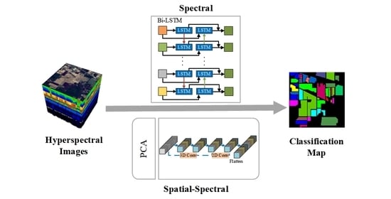
In summary, sufficiently exploiting features of HSI data and minimizing computational burden are the keys to HSI classification. This paper proposes a joint unified network operating in the spatial–spectral domain for the HSI classification. The network uses three layers of 3-D convolution for extracting the spatial–spectral feature of HSI, and subsequently adds a layer of 2-D convolution to further extract spatial features. For spectral feature extraction, this network treats all spectral bands as a sequence of images and enhances the interactions between spectral bands using Bi-LSTM. Finally, two fully connected (FC) layers are combined and use the softmax function for classification, which forms a unified neural network. We list the major contributions of our proposed method.
  • A Bi-LSTM framework based on band grouping is proposed for extracting spectral features. Bi-LSTM can obtain better performance in learning contextual features between adjacent spectral bands. In contrast to the general recurrent neural network, this framework can better adapt to a deeper network for HSI classification.
  • The proposed method adopts 3-D CNN for extracting the spatial–spectral features. To reduce the computational complexity of the whole framework, PCA is used before the convolutional layer of the 3-D CNN to reduce the data dimensionality.
  • A unified framework named the Bi-LSTM-CNN is proposed which integrates two subnetworks into a unified network by sharing the loss function. In addition, the framework adds the auxiliary loss function, which balances the effects of spectral and spatial-spectral features for the classification results to increase the classification accuracy.
The structure of the remaining part is as follows. Section 2 describes long short-term memory (LSTM), a 3-D CNN, and the framework of the Bi-LSTM-CNN. Section 3 introduces the HSI datasets, experimental configuration, and experimental results. Section 4 provides a detailed analysis and interpretation of the experimental results. Finally, conclusions are summarized in Section 5.

2. Materials and Methods

2.1. Related Work

2.1.1. LSTM

Some tasks need to consider the information of previous and subsequent inputs in processing the current input. RNNs can solve these problems and handle the spectral contextual information of an HSI. Figure 1 shows the architecture of an RNN. Given a series of values x ( 1 ) , x ( 2 ) , , x ( t ) as input data, the formula for each cell structure in the RNN network is shown as Equations (1) and (2):
h ( t ) = tan h ( W h ( t 1 ) + U x ( t ) + b a ) ,
O ( t ) = V h ( t ) + b o ,
where W , U , V denote the weight matrices that represent the relation of two nodes. In detail, W connects the previously hidden node and the currently hidden node, U connects the input node and the hidden node, and V connects the hidden node and the output node. Vectors b a and b o are bias vectors. At time t , x ( t ) represents the input value, h ( t ) represents the hidden value, and O ( t ) represents the output value. The tanh is a nonlinear activation function. The initialization value of h ( 0 ) in Equation (1) is set to zero. Equation (1) indicates that the output is jointly determined by the input x ( t ) at time t and the h ( t 1 ) at time t 1 . As | W | < 1 or | W | > 1 , h ( t ) will be closer to infinity or zero as time increases. This will cause the gradient to disappear or explode in the backpropagation phase. In other words, when the relevant information is very far from the current location, RNN will not utilize this information effectively. RNN cannot solve the problem of long-term dependence.
The LSTM network is proposed to solve this problem. Through the gating mechanism, the LSTM not only remembers past information but also filters some unimportant information. The LSTM is effective in solving the long dependency problem in the RNNs.
The architecture of LSTM is shown in Figure 2. The memory cell is a critical component of the LSTM, replacing the hidden unit of the RNNs. The cell state runs throughout the cell, but it has few branches to ensure information flows unchanged throughout the RNNs. The LSTM network has a structure called a gate, which can delete or add information about the cell state. The gate is combined by the Hadamard product operation and the sigmoid function and can filter which information is allowed to pass. The LSTM has three gates: the input gate, which determines how the previous memory is combined with the new input information; the output gate, which controls if the state of the cell at the next time step will affect other neurons; and the forget gate, which regulates the cell state, causing the cell to forget or remember a previous state. The candidate cell value stores updated information from the output of the input gate operation. At time t , the forward propagation of the LSTM is defined as Equations (3)–(8).
Input gate:
i ( t ) = σ ( W i x ( t ) + U i h ( t 1 ) + b i ) ,
Forget gate
f ( t ) = σ ( W f x ( t ) + U f h ( t 1 ) + b f ) ,
Output gate
o ( t ) = σ ( W o x ( t ) + U 0 h ( t 1 ) + b o ) ,
Candidate cell value
c ˜ ( t ) = tan h ( W c x ( t ) + U c h ( t 1 ) + b c ) ,
Cell state
c ( t ) = i ( t ) c ˜ ( t 1 ) + f ( t ) c ( t 1 ) ,
LSTM output
h ( t ) = o ( t ) tan h ( c ( t ) ) ,
where σ denotes the logistic sigmoid function and ∗ represents the Hadamard product operation. The matrices W i , W f , W o , W c , U i , U f , U o , and U c are weight matrices. The vectors b i , b f , b o , and b c are bias vectors.

2.1.2. CNN

CNNs are being applied with great success in many research areas. A CNN can extract various kinds of features from an image, such as color, texture, shape, and topology, so it has the advantage of processing 2-D images, such as identifying displacement, scaling, and other forms of distortion invariance. Similar to biological neural networks, the structure of the weight-sharing network of CNNs decreases the number of parameters, thus decreasing the complexity of the network model.
CNNs include 1-D CNN, 2-D CNN, and 3-D CNN. The 1-D CNN is mainly adopted for sequence data processing; the 2-D CNN is usually adopted for image recognition; the 3-D CNN is mainly used for medical image and video data recognition. A CNN consists of three structures: convolution layer, activation function, and pooling layer. There are no pooling layers in some CNNs. In detail, the purpose of the convolutional layer is for the extraction of the input data features; with more convolutional layers, the extracted features are more complex. The activation function increases the nonlinearity of the neural network model. The pooling layer preserves the main features while decreasing the number of parameters and calculations, preventing overfitting and improving model generalization. The schematic diagrams of the 2-D convolution and 3-D convolution are shown in Figure 3.

2.2. Framework of Proposed Method

The proposed Bi-LSTM-CNN network is based on the combination of Bi-LSTM and 3-D CNN for HSI classification. The method consists of two main parts—one for extracting spectral features through Bi-LSTM on the raw data and the other for extracting spatial-spectral features using 3-D CNN after the PCA dimension reduction on the data. To optimize the parameters of two subnetworks simultaneously, we concatenate the last of the FC layers of the Bi-LSTM and 3-D CNN to form a new FC layer, after which a softmax function is added. In this framework, the dimensionality of the raw data is decreased by the PCA to minimize the computational effort of 3-D convolution, and Bi-LSTM manages the original data to compensate for the spectral loss after dimensionality reduction. In addition, Bi-LSTM can better handle the contextual information of the spectra and fully exploit the spectral features of the HSI. After the last FC layer of each subnetwork, auxiliary functions are added to balance the contribution of the two subnetworks to the whole framework. The framework diagram of the Bi-LSTM-CNN is shown in Figure 4.

2.2.1. Bi-LSTM

In Section 2.1.1, we discussed the use of LSTM to process continuous HSI data and extract spectral information. The LSTM can retain only previous input information through cell states because it cannot access future input information. To handle this problem, we propose to extract spectral information using Bi-LSTM instead of LSTM. Unlike LSTM, Bi-LSTM preserves both latter and previous information. Additionally, Bi-LSTM shows accurate results with a better understanding of the context.
The Bi-LSTM network focuses on spectral contextual information. In general, the Bi-LSTM network inputs one band at a time step. However, HSI has hundreds of bands, making the Bi-LSTM network too deep to obtain a robust network under the condition of limited HSI samples. Therefore, the strategy used to group the spectral bands is crucial to improve HSI classification results. In Bi-LSTM, t denotes the number of groups; n denotes the number of bands; and m = f l o o r ( n / t ) represents the sequence length of each group, where f l o o r ( x ) denotes rounding down x . Z = [ Z 1 , Z 2 , Z i , Z n ] is the spectral vectors per pixel in the HSI, where Z i is the reflectance value of the i th band. The grouping strategy is shown as Equation (9):
x ( 1 ) = [ Z 1 , Z 1 + t , Z 1 + t ( m 1 ) ] x ( 2 ) = [ Z 2 , Z 2 + t , Z 2 + t ( m 1 ) ] x ( i ) = [ Z i , Z i + t , Z i + t ( m 1 ) ] x ( t ) = [ Z t , Z 2 t , Z t m ] ,
where x ( i ) is the i th group. In this strategy, there will be a relative shortening of the spectral distance between different groups, and most of the spectral range will be covered.
The framework diagram of the Bi-LSTM is shown in Figure 5. The Bi-LSTM contains information about the forward and backward of the input sequence. At time t of the input sequence, the forward LSTM layer contains information before time t , while the backward LSTM layer contains information after time t . The vectors output from the two LSTM layers are processed using concatenation. In Bi-LSTM, the colored squares represent each grouping. Each blue LSTM square represents an LSTM unit, and the red and green arrows indicate the forward LSTM and the backward LSTM, respectively, and the two LSTMs pass the information along the arrow direction. Meanwhile, the forward LSTM and the backward LSTM have the same input data.

2.2.2. 3-D CNN

The 3-D CNN has unique advantages in processing spatial-spectral features. Since there are many bands in an HSI, the 3-D convolution has a large computational complexity when extracting spatial-spectral features, which influences the efficiency of HSI classification. Therefore, in the Bi-LSTM-CNN, the 3-D CNN is used for the HSI after PCA dimensionality reduction to reduce the computational complexity.
HSI is denoted by X R W × H × B , where X represents the original data, W and H represent the width and the height, respectively, and B denotes the number of spectral bands. Each HSI pixel in X contains a one-hot label vector Y = ( y 1 , y 2 , y 3 , , y C ) R 1 × 1 × C and a value in each of the B spectral bands, where C denotes the land-cover categories. During the convolution operation, to remove the spectral correlation and decrease the computational costs, the number of spectral bands is decreased from B to P by the PCA, while keeping the W and H of the spatial dimension constant. The spectral bands are reduced, but the essential spatial information for HSI classification is preserved. We create the 3-D patches centered on each pixel and extract adjacent regions of size w × w × P , where w × w denotes the size of the window and P denotes the number of first principal components that have been reserved by the PCA. The label of the central pixel decides the truth labels of the patches. The dataset is represented by X P R M × w × w × P , where M represents the number of samples.
To achieve the spatial-spectral feature maps in the 3-D CNN, 3-D convolution is executed three times. Considering the crucial role of 2-D convolution in spatial information extraction, we apply 2-D convolution to increase the spatial feature maps before the flatten layer. To prevent overfitting and to improve the generalization of this model, the dropout is applied once after each FC layer. The structure of the 3-D CNN is shown in Figure 6.

2.2.3. Loss Function

In this framework, we adopt the softmax function after the final FC layer to determine the probability distributions over the pixel classes. In addition, to increase the nonlinearity and accelerate the convergence of the Bi-LSTM-CNN, we adopt the rectified linear units (ReLU) function after each layer.
To better train the parameters of the whole framework, after the final FC layer in the Bi-LSTM and the 3-D CNN, we adopt the auxiliary loss function. The complete loss function is defined as Equations (10)–(13):
L j o i n t = 1 m i = 1 m [ y i log ( y ^ i j o i n t ) + ( 1 y i ) log ( 1 y ^ i j o i n t ) ] ,
L B i - L S T M = 1 m i = 1 m [ y i log ( y ^ i B i - L S T M ) + ( 1 y i ) log ( 1 y ^ i B i - L S T M ) ] ,
L C N N = 1 m i = 1 m [ y i log ( y ^ i C N N ) + ( 1 y i ) log ( 1 y ^ i C N N ) ] ,
L = L j o i n t + L B i - L S T M + L C N N ,
where L represents the loss function, and y ^ i and y i refer to the predicted label and true label for the i th training sample, respectively. The superscript j o i n t , B i - L S T M , and C N N denote the whole framework, the Bi-LSTM network, and the 3-D CNN, respectively. The variable m denotes the number of the training sample. The parameters of the Bi-LSTM-CNN were optimized by the mini-batch stochastic gradient descent (SGD) algorithm.
The implementation procedure of the proposed Bi-LSTM-CNN method is shown in Algorithm 1.
Algorithm 1. Bi-LSTM-CNN procedure
Input
(1)
HSI with labels.
(2)
The size of the patch w , the number of retained principal components P .
Step 1 
For each pixel in the HSI, use Equation (9) to divide the hyperspectral cube into t sequences as the input of the Bi-LSTM network.
Step 2 
Retain the first P principal components with PCA. Extract a patch of size w × w × P in the neighborhood of each pixel after the reduced-dimensional HSI as the input of the 3-D CNN.
Step 3 
Initialize the weights in the Bi-LSTM-CNN by assigning random values that follow a Gaussian distribution, where the mean, standard deviation, and bias terms are initialized to 0, 0.1, and 0, respectively.
Step 4 
Import training samples into the Bi-LSTM-CNN. Bi-LSTM and 3-D CNN extract the spectral features and spatial-spectral features for HSI, respectively. Then, softmax is applied to classify the extracted features. Finally, the mini-batch SGD algorithm is exploited to optimize the parameters of the Bi-LSTM-CNN, and the parameters are adjusted by backpropagation to obtain the optimal parameters.
Step 5 
For each pixel in the HSI, input the corresponding data from Step 1 and Step 2 to the Bi-LSTM-CNN to obtain the predicted value for the HSI.
Output
   Prediction results for each pixel of HSI.

3. Results

In this section, three open HSI datasets (the three datasets are available at http://www.ehu.eus/ccwintco/index.php/Hyperspectral_Remote_Sensing_Scenes accessed on 14 November 2020) are evaluated in the performance of the Bi-LSTM-CNN by applying three evaluation metrics, comprising overall accuracy (OA), average accuracy (AA), and kappa coefficient (Kappa).

3.1. Dataset Description and Training Details

The Indian Pines (IP) is an image acquired by the AVIRIS sensor in 1992 from the Agricultural and Forestry Hyperspectral Experiment site in northwestern Indiana. The dataset is an agricultural region with geometrically regular crop areas but irregular forest areas. The dataset is the size of 145 × 145 and has 224 spectral reflectance bands. The spatial resolution of each pixel is 20 m . Of these, 24 spectral bands were excluded because they covered the water absorption region; the wavelength range of the retained 200 bands is 0.4–2.5   μ m . The available samples were divided into 16 categories, representing approximately half of the total data. The false-color composite image and the ground-truth map correspond to in Figure 7a,b respectively. In the experiment, the dataset was selected randomly in the labeled parts from each category, and the ratio of the training and testing set was 1:9. Table 1 exhibits the details of the sample, as well as the corresponding colors of the ground-truth map.
The University of Pavia (PU) campus in northern Italy was gathered by the ROSIS-03 sensor in 2001. This scene has a size of 610 × 340 × 115 and a wavelength range of 0.43–0.86 μ m . The spatial resolution of each pixel is 1.3 m . This scene contained nine categories and 103 spectral bands after 12 noisy bands were discarded. The false-color composite image and the ground-truth map correspond to in Figure 8a,b respectively. Table 2 exhibits the details of the sample, as well as the corresponding colors of the ground-truth map. In the labeled pixels from the PU, only 5% were used as the training set and the rest as the testing set.
The Salinas Valley (SV) scene is an image of the Salinas Valley, California, collected by the AVIRIS sensor. This scene forms a cube of dimension 512 × 217 × 224, and the spatial resolution of each pixel is 3.7 m . Similar to the IP dataset, after discarding 20 water absorption and noise bands, only 204 bands remained. This scene included 16 different agriculture crop categories. The false-color composite image and the ground-truth map correspond to in Figure 9a,b respectively. Table 3 exhibits the details of the sample, as well as the corresponding colors of the ground-truth map. Among the labeled pixels of this scene, only 5% were used as the training set and the rest as the testing set. In the above three datasets, the data of all training sets are randomly selected.

3.2. Experimental Configuration

All the experiments were run with an NVIDIA GTX 1070 GPU and an Inter i7-6700 3.40-GHz CPU with 32 GB of RAM. We performed randomized training and test data replication 10 times for each test. Based on several experiments, we chose 0.0001 as the best learning rate. To optimize the Bi-LSTM-CNN, we adopted the mini-batch SGD algorithm, with a batch size of 128. In the Bi-LSTM, the spectral bands are divided into three groups.
In Table 4, it is evident that the Bi-LSTM-CNN obtained the optimal results when the input window of the 3-D patches was 25 × 25. Table 5 shows the effect of P on the classification results in the IP dataset. When P is 30, the classification results are best. If P keeps increasing, the number of network parameters will increase sharply. Therefore, the input size of the 3-D patches was 25 × 25 × 30. In Figure 10, the curves of classification accuracy with epochs during training over IP, PU, and SV datasets. When the epoch is 100, the classification accuracy was close to 1, but there was still instability. The classification accuracy was stable when the epoch reached 300, so the epoch of the Bi-LSTM-CNN was adopted 300. The parameters for the proposed Bi-LSTM-CNN method on the IP dataset are shown in Table 6.

3.3. Classification Results

In this paper, we compared the Bi-LSTM-CNN with some state-of-the-art methods, which are CNN1D, CNN2D, and CNN3D [56], SSUN [57], and HybridSN [58]. CNN1D, CNN2D, and CNN3D used 1-D convolution, 2-D convolution, and 3-D convolution, respectively. SSUN used an LSTM and a multiscale CNN to extract spectral and spatial features for implementing spatial and spectral joints. HybridSN adopted a mixture of 3-D convolution and 2-D convolution to extract spatial-spectral features with mainly spatial information. All the comparison methods were run in the same environment.
Table 7, Table 8 and Table 9 show the results acquired by six methods on the IP (10% of the total dataset), PU (5%), and SV (5%), including OA, AA, Kappa, testing time, accuracy for each class. These are the result of running on the testing set. CNN1D had the worst classification results. In detail, all three evaluation metrics (OA, AA, and Kappa) of CNN1D were lower than the other methods. The accuracy of each class is the lowest among the six methods. CNN2D had better classification results than CNN1D, but still had a large drawback with other methods. Among the remaining methods, each method achieves the best results in some classes. Specifically, the Bi-LSTM-CNN obtained higher performance than other methods on OA, AA, Kappa. In addition, the Bi-LSTM-CNN obtains the highest accuracy in most of classes. The testing time of CNN1D, CNN2D, SSUN are less than other comparison methods.
The classification maps of the six methods in the three datasets are shown in Figure 7, Figure 8 and Figure 9. These Figures show the prediction results of the six methods for all labeled samples. It is obvious that the classification maps of CNN1D and CNN2D have a large amount of salt and pepper noise. As the remaining four methods used spatial and spectral information, the classification map approximates more closely to the ground-truth map. In particular, the Bi-LSTM-CNN has very few pixel points that are different from the ground-truth map.

4. Discussion

In the experiment result, it is obvious that the Bi-LSTM-CNN significantly outperforms the other methods. The OA of the CNN1D method did not exceed 94% in all the considered datasets. Since the input data of CNN1D is a 1-D vector, spatial information of the input data is lost, resulting in the worst classification results of CNN1D among all methods. The CNN2D model considers the spatial information, which makes the classification results an improvement compared to CNN1D. Thus, it shows that spatial information is critical for HSI classification.
However, the CNN2D model has problems, which usually result in degraded shapes of some objects and materials. The union of spatial and spectral information can address this issue, and the other methods (CNN3D, SSUN, HybridSN, and Bi-LSTM-CNN) all achieve more similar classification results to the corresponding ground-truth maps. The SSUN model extracts spatial and spectral features separately, which are integrated and then sent to the classifier for classification. As spatial features dominate the classification results, SSUN is unable to effectively balance the two features, thus resulting in a little contribution of spectral features to the classification results. The CNN3D model directly extracts the spatial-spectral features of the HSI, but to decline the computational complexity of the convolutional layers, the PCA dimensionality reduction is performed on the input data. Hence, a small amount of spectral information is lost. Despite this, CNN3D still spends a lot of time in the testing phase on the PU and SV dataset compared to HybridSN and Bi-LSTM-CNN.
The HybridSN model replaces the final 3-D convolutional layer with 2-D convolution, decreasing the number of parameters in the network while maintaining accuracy. However, in the PU dataset experiments, the OA of the HybridSN model is lower than the CNN3D model, and the generalizability of the HybridSN method is slightly worse. In the Bi-LSTM-CNN, the lack of 3-D CNN processing spectral information is compensated, and the experimental results after adding Bi-LSTM are significantly better than the other methods.
In the classes with a small number of samples, the Bi-LSTM-CNN method also obtains better classification results. In the IP dataset, due to the very small number of labeled samples in some classes, the number of available training samples is extremely small. For example, the number of samples for C1, C7, C9, C16 is not more than ten, which greatly increases the learning difficulty for these classes. Except for C1, the best classification accuracy is obtained for several other categories. Except for C1, the Bi-LSTM-CNN method obtains a higher OA in the other classes than other methods. In the PU and SV datasets, the number of training samples for each class is sufficient for the Bi-LSTM-CNN method, although there is a large difference in the number of samples for different classes.

5. Conclusions

This paper proposed a unified network framework that contained a band-grouping-based Bi-LSTM network and a 3-D CNN for HSI classification. In this network, Bi-LSTM can extract high-quality spectral features considering complete spectral contextual information, which compensates for the shortcomings of the 3-D CNN. The Bi-LSTM-CNN network is able to harness the strengths of both subnetworks by using auxiliary loss functions. Compared with the model using only 3-D CNN, the Bi-LSTM-CNN can obtain better classification results by adding a few parameters. In the PU and SV datasets, we validated the performance of the model using less training data (5%). The experimental results showed that the Bi-LSTM-CNN method significantly improved the accuracy of HSI classification. In future work, we will either replace the LSTM with the Gated Recurrent Unit to improve the speed of the network or use the optimized 3-D CNN to further improve the HSI classification results.

Author Contributions

Methodology, software and conceptualization, J.Y. and Q.C.; modification and writing—review and editing, C.Q.; investigation and data curation, J.Q. All authors have read and agreed to the published version of the manuscript.

Funding

This research was funded by the Henan Province Science and Technology Breakthrough Project, grant number 212102210102 and 212102210105.

Acknowledgments

The authors would like to thank the editors and reviewers for their advice.

Conflicts of Interest

The authors declare no conflict of interest.

Abbreviations

The abbreviations in this paper are as follows:
HSIHyperspectral Image
Bi-LSTMBiderectional Long Short-Term Memory
CNNConvolutional Neural Network
SVMSupport Vector Machine
KNNK-Nearest Neighbor
SAEStacked Auto-Encoder
DBNDeep Belief Network
RNNRecurrent Neural Network
GANGenerative Adversarial Network
AEAuto-Encoder
PCAPrincipal Component Analysis
FCFully Connected
LSTMLong Short-Term Memory
ReLURectified Linear Unit
OAOverall Accuracy
AAAverage Accuracy
KappaKappa Coefficient
PCPrincipal Component
IPIndian Pines
PUUniversity of Pavia

References

  1. Chang, C.I. Hyperspectral Imaging: Techniques for Spectral Detection and Classification; Springer: Berlin/Heidelberg, Germany, 2003; Volume 1, pp. 1–63. [Google Scholar]
  2. Gu, Y.; Chanussot, J.; Jia, X.; Benediktsson, J.A. Multiple Kernel Learning for Hyperspectral Image Classification: A Review. IEEE Trans. Geosci. Remote. Sens. 2017, 55, 6547–6565. [Google Scholar] [CrossRef]
  3. Li, S.; Song, W.; Fang, L.; Chen, Y.; Ghamisi, P.; Benediktsson, J.A. Deep Learning for Hyperspectral Image Classification: An Overview. IEEE Trans. Geosci. Remote Sens. 2019, 57, 6690–6709. [Google Scholar] [CrossRef] [Green Version]
  4. Sun, L.; Wu, F.; He, C.; Zhan, T.; Liu, W.; Zhang, D. Weighted Collaborative Sparse and L1/2 Low-Rank Regularizations with Superpixel Segmentation for Hyperspectral Unmixing. IEEE Geosci. Remote Sens. Lett. 2020, 1–5. [Google Scholar] [CrossRef]
  5. Shaw, G.; Manolakis, D. Signal processing for hyperspectral image exploitation. IEEE Signal Process. Mag. 2002, 19, 12–16. [Google Scholar] [CrossRef]
  6. Landgrebe, D.; Landgrebe, D. Hyperspectral image data analysis. IEEE Signal Process. Mag. 2002, 19, 17–28. [Google Scholar] [CrossRef]
  7. Schmid, T.; Koch, M.; Gumuzzio, J. Multisensor approach to determine changes of wetland characteristics in semiarid envi-ronments (Central Spain). IEEE Trans. Geosci. Remote Sens. 2005, 43, 2516–2525. [Google Scholar] [CrossRef]
  8. Ghiyamat, A.; Shafri, H.Z.M. A review on hyperspectral remote sensing for homogeneous and heterogeneous forest bio-diversity assessment. Int. J. Remote Sens. 2010, 31, 1837–1856. [Google Scholar] [CrossRef]
  9. Pontius, J.; Martin, M.; Plourde, L.; Hallett, R. Ash decline assessment in emerald ash borer-infested regions: A test of tree-level, hyperspectral technologies. Remote Sens. Environ. 2008, 112, 2665–2676. [Google Scholar] [CrossRef]
  10. Cloutis, E.A. Review Article Hyperspectral geological remote sensing: Evaluation of analytical techniques. Int. J. Remote Sens. 1996, 17, 2215–2242. [Google Scholar] [CrossRef]
  11. Hou, Y.; Zhu, W.; Wang, E. Hyperspectral Mineral Target Detection Based on Density Peak. Intell. Autom. Soft Comput. 2019, 25, 805–814. [Google Scholar] [CrossRef]
  12. Lanthier, Y.; Bannari, A.; Haboudane, D.; Miller, J.R.; Tremblay, N. Hyperspectral Data Segmentation and Classification in Precision Agriculture: A Multi-Scale Analysis. IEEE Trans. Geosci. Remote Sens. 2008, 2, 585. [Google Scholar] [CrossRef]
  13. Boggs, J.L.; Tsegaye, T.D.; Coleman, T.L.; Reddy, K.C.; Fahsi, A. Relationship Between Hyperspectral Reflectance, Soil Nitrate-Nitrogen, Cotton Leaf Chlorophyll, and Cotton Yield: A Step Toward Precision Agriculture. J. Sustain. Agric. 2003, 22, 5–16. [Google Scholar] [CrossRef]
  14. Briottet, X.; Boucher, Y.G.; Dimmeler, A.; Malaplate, A.; Cini, A.; Diani, M.; Bekman, H.H.P.T.; Schwering, P.B.W.; Skauli, T.; Kasen, I.; et al. Military applications of hyperspectral imagery. In Defense and Security Symposium; International Society for Optics and Photonics: Bellingham, WA, USA, 2006; Volume 6239, pp. 1–8. [Google Scholar]
  15. He, C.; Sun, L.; Huang, W.; Zhang, J.; Zheng, Y.; Jeon, B. TSLRLN: Tensor subspace low-rank learning with non-local prior for hyperspectral image mixed denoising. Signal Process. 2021, 184, 108060. [Google Scholar] [CrossRef]
  16. Sun, L.; He, C.; Zheng, Y.; Tang, S. SLRL4D: Joint restoration of subspace low-rank learning and non-local 4-D transform filtering for hyperspectral image. Remote Sens. 2020, 12, 2979. [Google Scholar] [CrossRef]
  17. Li, J.; Bioucas-Dias, J.; Plaza, A. Spectral–Spatial Hyperspectral Image Segmentation Using Subspace Multinomial Logistic Regression and Markov Random Fields. IEEE Trans. Geosci. Remote Sens. 2011, 50, 809–823. [Google Scholar] [CrossRef]
  18. Melgani, F.; Bruzzone, L. Classification of hyperspectral remote sensing images with support vector machines. IEEE Trans. Geosci. Remote Sens. 2004, 42, 1778–1790. [Google Scholar] [CrossRef] [Green Version]
  19. Huang, W.; Huang, Y.; Wang, H.; Liu, Y.; Shim, H.J. Local binary patterns and superpixel-based multiple kernels for hy-perspectral image classification. IEEE J. Sel. Top. Appl. Earth Obs. Remote Sens. 2020, 13, 4550–4563. [Google Scholar] [CrossRef]
  20. Ye, Q.; Zhao, H.; Li, Z.; Yang, X.; Gao, S.; Yin, T.; Ye, N. L1-Norm Distance Minimization-Based Fast Robust Twin Support Vector kk -Plane Clustering. IEEE Trans. Neural Netw. Learn. Syst. 2017, 29, 4494–4503. [Google Scholar] [CrossRef]
  21. Kramer, O. Dimensionality Reduction with Unsupervised Nearest Neighbors; Springer: Berlin/Heidelberg, Germany, 2013; Volume 51, pp. 13–23. [Google Scholar]
  22. Zhong, Y.; Zhang, L. An Adaptive Artificial Immune Network for Supervised Classification of Multi-/Hyperspectral Remote Sensing Imagery. IEEE Trans. Geosci. Remote Sens. 2011, 50, 894–909. [Google Scholar] [CrossRef]
  23. Fu, L.; Li, Z.; Ye, Q.; Yin, H.; Liu, Q.; Chen, X.; Fan, X.; Yang, W.; Yang, G. Learning Robust Discriminant Subspace Based on Joint L2, p- and L2, s-Norm Distance Metrics. IEEE Trans. Neural Netw. Learn. Syst. 2020, 1–15. [Google Scholar] [CrossRef]
  24. Ye, Q.; Li, Z.; Fu, L.; Zhang, Z.; Yang, W.; Yang, G. Nonpeaked Discriminant Analysis for Data Representation. IEEE Trans. Neural Netw. Learn. Syst. 2019, 30, 3818–3832. [Google Scholar] [CrossRef]
  25. Ye, Q.; Yang, J.; Liu, F.; Zhao, C.; Ye, N.; Yin, T. L1-Norm Distance Linear Discriminant Analysis Based on an Effective Iterative Algorithm. IEEE Trans. Circuits Syst. Video Technol. 2018, 28, 114–129. [Google Scholar] [CrossRef]
  26. Jay, S.; Guillaume, M. A novel maximum likelihood based method for mapping depth and water quality from hyperspectral remote-sensing data. Remote Sens. Environ. 2014, 147, 121–132. [Google Scholar] [CrossRef]
  27. Ghamisi, P.; Maggiori, E.; Li, S.; Souza, R.; Tarablaka, Y.; Moser, G.; De Giorgi, A.; Fang, L.; Chen, Y.; Chi, M.; et al. New Frontiers in Spectral-Spatial Hyperspectral Image Classification: The Latest Advances Based on Mathematical Morphology, Markov Random Fields, Segmentation, Sparse Representation, and Deep Learning. IEEE Geosci. Remote Sens. Mag. 2018, 6, 10–43. [Google Scholar] [CrossRef]
  28. He, L.; Li, J.; Liu, C.; Li, S. Recent Advances on Spectral–Spatial Hyperspectral Image Classification: An Overview and New Guidelines. IEEE Trans. Geosci. Remote Sens. 2017, 56, 1579–1597. [Google Scholar] [CrossRef]
  29. Li, S.; Lu, T.; Fang, L.; Jia, X.; Benediktsson, J.A. Probabilistic Fusion of Pixel-Level and Superpixel-Level Hyperspectral Image Classification. IEEE Trans. Geosci. Remote Sens. 2016, 54, 7416–7430. [Google Scholar] [CrossRef]
  30. Lu, T.; Li, S.; Fang, L.; Jia, X.; Benediktsson, J.A. From Subpixel to Superpixel: A Novel Fusion Framework for Hyperspectral Image Classification. IEEE Trans. Geosci. Remote Sens. 2017, 55, 4398–4411. [Google Scholar] [CrossRef]
  31. Mohanapriya, N.; Kalaavathi, B. Adaptive Image Enhancement using Hybrid Particle Swarm Optimization and Watershed Segmentation. Intell. Autom. Soft Comput. 2018, 25, 1–11. [Google Scholar] [CrossRef]
  32. Huang, W.; Xu, Y.; Hu, X.; Wei, Z. Compressive Hyperspectral Image Reconstruction Based on Spatial-Spectral Residual Dense Network. IEEE Geosci. Remote. Sens. Lett. 2019, 17, 1–5. [Google Scholar] [CrossRef]
  33. Mao, W.L.; Hung, C.W.; Huang, H.Y. Modified PSO Algorithm on Recurrent Fuzzy Neural Network for System Identification. Intell. Autom. Soft Comput. 2019, 25, 329–341. [Google Scholar] [CrossRef]
  34. Zhang, X.; Lu, W.; Li, F.; Peng, X.; Zhang, R. Deep Feature Fusion Model for Sentence Semantic Matching. Comput. Mater. Contin. 2019, 61, 601–616. [Google Scholar] [CrossRef]
  35. Harsanyi, J.C.; Chang, C.I. Hyperspectral image classification and dimensionality reduction: An orthogonal subspace projection approach. IEEE Trans. Geosci. Remote Sens. 1994, 32, 779–785. [Google Scholar] [CrossRef] [Green Version]
  36. Wu, H.; Liu, Q.; Liu, X. A Review on Deep Learning Approaches to Image Classification and Object Segmentation. Comput. Mater. Contin. 2019, 60, 575–597. [Google Scholar] [CrossRef] [Green Version]
  37. Girshick, R.; Donahue, J.; Darrell, T.; Malik, J. Rich Feature Hierarchies for Accurate Object Detection and Semantic Segmentation. In Proceedings of the 2014 IEEE Conference on Computer Vision and Pattern Recognition, Columbus, OH, USA, 23–28 June 2014; pp. 580–587. [Google Scholar]
  38. Du, B.; Zhang, L. A Discriminative Metric Learning Based Anomaly Detection Method. IEEE Trans. Geosci. Remote. Sens. 2014, 52, 6844–6857. [Google Scholar] [CrossRef]
  39. Huang, W.; Li, G.; Chen, Q.; Ju, M.; Qu, J. CF2PN: A Cross-Scale Feature Fusion Pyramid Network Based Remote Sensing Target Detection. Remote Sens. 2021, 13, 847. [Google Scholar] [CrossRef]
  40. Manolakis, D.; Shaw, G.; Manolakis, D.; Shaw, G. Detection algorithms for hyperspectral imaging applications. IEEE Signal Process. Mag. 2002, 19, 29–43. [Google Scholar] [CrossRef]
  41. Bordes, A.; Glorot, X.; Weston, J.; Bengio, Y. Joint Learning of Words and Meaning Representations for Open-Text Semantic Parsing. In Proceedings of the Artificial Intelligence and Statistics, La Palma, Spain, 21–23 April 2012; pp. 127–135. [Google Scholar]
  42. Chen, Y.; Zhao, X.; Jia, X. Spectral–Spatial Classification of Hyperspectral Data Based on Deep Belief Network. IEEE J. Sel. Top. Appl. Earth Obs. Remote Sens. 2015, 8, 2381–2392. [Google Scholar] [CrossRef]
  43. Suk, H.-I.; Lee, S.-W.; Shen, D. Latent feature representation with stacked auto-encoder for AD/MCI diagnosis. Brain Struct. Funct. 2015, 220, 841–859. [Google Scholar] [CrossRef]
  44. Mou, L.; Ghamisi, P.; Zhu, X.X. Deep Recurrent Neural Networks for Hyperspectral Image Classification. IEEE Trans. Geosci. Remote Sens. 2017, 55, 3639–3655. [Google Scholar] [CrossRef] [Green Version]
  45. Seydgar, M.; Alizadeh Naeini, A.; Zhang, M.; Li, W.; Satari, M. 3-D convolution-recurrent networks for spectral-spatial clas-sification of hyperspectral images. Remote Sens. 2019, 11, 883. [Google Scholar] [CrossRef] [Green Version]
  46. Ma, X.; Fu, A.; Wang, J.; Wang, H.; Yin, B. Hyperspectral Image Classification Based on Deep Deconvolution Network with Skip Architecture. IEEE Trans. Geosci. Remote Sens. 2018, 56, 4781–4791. [Google Scholar] [CrossRef]
  47. Wang, J.; Song, X.; Sun, L.; Huang, W.; Wang, J. A novel cubic convolutional neural network for hyperspectral image classi-fication. IEEE J. Sel. Top. Appl. Earth Obs. Remote Sens. 2020, 13, 4133–4148. [Google Scholar] [CrossRef]
  48. Zhong, Z.; Li, J.; Luo, Z.; Chapman, M. Spectral–Spatial Residual Network for Hyperspectral Image Classification: A 3-D Deep Learning Framework. IEEE Trans. Geosci. Remote Sens. 2017, 56, 847–858. [Google Scholar] [CrossRef]
  49. Wang, G.; Ren, P. Hyperspectral Image Classification with Feature-Oriented Adversarial Active Learning. Remote Sens. 2020, 12, 3879. [Google Scholar] [CrossRef]
  50. Li, J. Active learning for hyperspectral image classification with a stacked autoencoders based neural network. In Proceedings of the 2015 7th Workshop on Hyperspectral Image and Signal Processing: Evolution in Remote Sensing (WHISPERS), Tokyo, Japan, 2–5 June 2015; pp. 1–4. [Google Scholar] [CrossRef]
  51. Guofeng, T.; Yong, L.; Lihao, C.; Chen, J. A DBN for hyperspectral remote sensing image classification. In Proceedings of the 2017 12th IEEE Conference on Industrial Electronics and Applications (ICIEA), Institute of Electrical and Electronics Engineers (IEEE). Siem Reap, Cambodia, 18–20 June 2017; pp. 1757–1762. [Google Scholar]
  52. Hu, W.; Huang, Y.; Wei, L.; Zhang, F.; Li, H.-C. Deep Convolutional Neural Networks for Hyperspectral Image Classification. J. Sens. 2015, 2015, 1–12. [Google Scholar] [CrossRef] [Green Version]
  53. Zhao, W.; Guo, Z.; Yue, J.; Zhang, X.; Luo, L. On combining multiscale deep learning features for the classification of hy-perspectral remote sensing imagery. Int. J. Remote Sens. 2015, 36, 3368–3379. [Google Scholar] [CrossRef]
  54. Chen, Y.; Jiang, H.; Li, C.; Jia, X.; Ghamisi, P. Deep Feature Extraction and Classification of Hyperspectral Images Based on Convolutional Neural Networks. IEEE Trans. Geosci. Remote Sens. 2016, 54, 6232–6251. [Google Scholar] [CrossRef] [Green Version]
  55. Liu, Q.; Zhou, F.; Hang, R.; Yuan, X. Bidirectional-Convolutional LSTM Based Spectral-Spatial Feature Learning for Hyperspectral Image Classification. Remote Sens. 2017, 9, 1330. [Google Scholar] [CrossRef] [Green Version]
  56. Paoletti, M.; Haut, J.; Plaza, J.; Plaza, A. Deep learning classifiers for hyperspectral imaging: A review. ISPRS J. Photogramm. Remote Sens. 2019, 158, 279–317. [Google Scholar] [CrossRef]
  57. Xu, Y.; Zhang, L.; Du, B.; Zhang, F. Spectral-Spatial Unified Networks for Hyperspectral Image Classification. IEEE Trans. Geosci. Remote Sens. 2018, 56, 1–17. [Google Scholar] [CrossRef]
  58. Roy, S.K.; Krishna, G.; Dubey, S.R.; Chaudhuri, B.B. HybridSN: Exploring 3-D–2-D CNN Feature Hierarchy for Hyperspectral Image Classification. IEEE Geosci. Remote Sens. Lett. 2020, 17, 277–281. [Google Scholar] [CrossRef] [Green Version]
Figure 1. RNN architecture.
Remotesensing 13 02353 g001
Figure 2. LSTM architecture.
Remotesensing 13 02353 g002
Figure 3. Schematic diagrams of (a) 2-D convolution and (b) 3-D convolution.
Remotesensing 13 02353 g003
Figure 4. Framework diagram of the Bi-LSTM-CNN.
Remotesensing 13 02353 g004
Figure 5. Bi-LSTM framework diagram.
Remotesensing 13 02353 g005
Figure 6. 3-D CNN framework diagram. Each convolutional layer is used with a ReLU function. The stride of each layer is 1.
Remotesensing 13 02353 g006
Figure 7. Classification maps for the IP dataset with 10% of training data. (a) False-color image, (b) Ground-truth map, (c) CNN1D, (d) CNN2D, (e) CNN3D, (f) SSUN, (g) HybridSN, (h) Bi-LSTM-CNN.
Remotesensing 13 02353 g007
Figure 8. Classification maps for the PU dataset with 10% of training data. (a) False-color image; (b) Ground-truth map; (c) CNN1D; (d) CNN2D; (e) CNN3D; (f) SSUN; (g) HybridSN; (h) Bi-LSTM-CNN.
Remotesensing 13 02353 g008
Figure 9. Classification maps for the SV dataset with 10% of training data. (a) False-color image; (b) Ground-truth map; (c) CNN1D; (d) CNN2D; (e) CNN3D; (f) SSUN; (g) HybridSN; (h) Bi-LSTM-CNN.
Remotesensing 13 02353 g009aRemotesensing 13 02353 g009b
Figure 10. In three datasets, classification accuracy for each epoch during training.
Remotesensing 13 02353 g010
Table 1. Details of the IP dataset.
Class NO.Class NameColorNumber of Training SamplesNumber of Testing SamplesTotal Number of Samples
C1Alfalfa 54146
C2Corn—no till 14312851428
C3Corn—min till 83747830
C4Corn 24213237
C5Grass/pasture 48435483
C6Grass/tree 73657730
C7Grass/pasture—mowed 32528
C8Hay—windrowed 48430478
C9Oats 21820
C10Soybeans—no till 97875972
C11Soybeans—min till 24522102455
C12Soybeans—clean till 59534593
C13Wheat 20185205
C14Woods 12611391265
C15Bldg-grass-tree-drives 39347386
C16Stone-steel towers 98493
Total1024922510,249
Table 2. Details of the PU dataset.
Class NO.Class NameColorNumber of Training SamplesNumber of Testing SamplesTotal Number of Samples
C1Asphalt 33262996631
C2Meadows 93317,71618,649
C3Gravel 10519942099
C4Trees 15329113064
C5Painted metal sheets 6712781345
C6Bare soil 25147785029
C7Bitumen 6712631330
C8Self-blocking bricks 18434983682
C9Shadows 47900947
Total213940,63742,776
Table 3. Details of the SV dataset.
Class NO.Class NameColorNumber of Training SamplesNumber of Testing SamplesTotal Number of Samples
C1Brocoli_green_weeds_1 10019092009
C2Brocoli_green_weeds_2 18635403726
C3Fallow 9918771976
C4Fallow_rough_plow 7013241394
C5Fallow_smooth 13425442678
C6Stubble 19837613959
C7Celery 17934003579
C8Grapes_untrained 56410,70711,271
C9Soil_vinyard_develop 31058936203
C10Corn_senesced_green_weeds 16431143278
C11Lettuce_romaine_4wk 5310151068
C12Lettuce_romaine_5wk 9618311927
C13Lettuce_romaine_6wk 46870916
C14Lettuce_romaine_7wk 5410161070
C15Vinyard_untrained 36469047268
C16Vinyard_vertical_trellis 9017171807
Total270751,42254,129
Table 4. Impact of the input window size of the 3-D patches on the performance.
WindowIPPUSV
OA (%)AA (%)Kappa × 100OA (%)AA (%)Kappa × 100OA (%)AA (%)Kappa × 100
10 × 1095.4193.0794.8696.3595.1895.1795.0197.5794.45
15 × 1597.9396.1197.6598.1597.3997.5597.7898.9197.53
20 × 2098.2997.6098.0499.0698.4298.7699.1499.5699.04
25 × 2598.6398.5098.4599.5699.2299.4299.8199.8399.84
Table 5. In the IP dataset, impact of the number of retained principal component on the performance.
P OA (%)AA (%)Kappa × 100 P OA (%)AA (%)Kappa × 100
1598.1397.7797.862598.5598.4698.35
2098.1897.8797.923098.6498.5098.45
Table 6. Parameters for the proposed Bi-LSTM-CNN method on the IP dataset.
Layer (Type)Output ShapeParam #
CNNInput (InputLayer)(25, 25, 30, 1)0
conv3d1 (Conv3D)(23, 23, 24, 8)512
conv3d2 (Conv3D)(21, 21, 20, 16)5776
conv3d3 (Conv3D)(19, 19, 18, 32)13856
reshape1 (Reshape)(19, 19, 576)0
conv2d1 (Conv2D)(17, 17, 64)331840
flatten1 (Flatten)(18496)0
dense1 (Dense)(256)4735232
BiLSTMInput (InputLayer)(3, 66)0
dropout1 (Dropout)(256)0
bidirectional1 (Bidirectional)(256)199680
dense2 (Dense)(128)32896
BiLSTMDense (Dense)(128)32896
dropout2 (Dropout)(128)0
concatenate1 (Concatenate)(256)0
JOINTDENSE (Dense)(128)32896
JOINTSOFTMAX (Dense)(16)2064
LSTMSOFTMAX (Dense)(16)2064
CNNSOFTMAX (Dense)(16)2064
Total params #: 5,391,776
Table 7. Classification results for the IP dataset using 10% of the available labeled data.
Class NO.CNN1DCNN2DCNN3DSSUNHybridSNBi-LSTM-CNN
C132.4469.5180.7399.5186.1996.10
C269.8491.1897.6896.9394.6394.93
C362.8290.9898.7098.3499.2698.90
C443.0587.1894.0897.5196.3297.93
C588.4889.9896.2596.9999.0498.99
C696.5997.4199.5398.8798.9399.30
C740.4087.2088.0097.20100.00100.00
C898.2898.8499.9899.8899.30100.00
C939.4457.2285.5678.3390.7496.11
C1067.3493.3497.1295.9498.6199.15
C1182.9295.3698.9098.4899.0099.50
C1273.1588.3194.4097.0895.8298.78
C1397.9597.2499.7898.4397.5799.72
C1494.0498.6499.7298.9099.7799.82
C1560.9891.5995.7697.5898.8099.79
C1683.4590.1296.5593.8191.6797.61
OA (%)78.8993.7397.9997.8998.0598.63
AA (%)71.5889.0195.1796.5396.6098.50
Kappa × 10074.8892.8597.7097.6097.7898.45
Testing time (s)0.360.613.491.194.545.34
Table 8. Classification results for the PU dataset using 5% of the available labeled data.
Class NO.CNN1DCNN2DCNN3DSSUNHybridSNBi-LSTM-CNN
C193.2299.4399.0298.5599.5999.59
C298.0199.8399.9999.8499.97100.00
C377.9997.4495.3995.5097.7797.19
C492.3397.4999.0499.1698.6399.29
C599.5799.8499.9999.6399.40100.00
C687.5388.78100.0099.5199.97100.00
C787.2499.2999.9996.1299.9498.97
C884.0797.4998.1998.6297.9698.28
C999.6695.8998.8898.7294.3299.67
OA (%)93.2098.0599.4899.0999.3899.56
AA (%)91.0797.5099.1698.4198.6199.22
Kappa × 10090.9497.4299.3198.7999.1999.42
Testing time (s)1.413.4014.634.457.2910.62
Table 9. Classification results for the SV dataset using 5% of the available labeled data.
Class NO.CNN1DCNN2DCNN3DSSUNHybridSNBi-LSTM-CNN
C199.2099.42100.0099.83100.00100.00
C299.9699.87100.0099.93100.00100.00
C398.9799.68100.0099.89100.00100.00
C499.2099.3199.6699.6899.9999.99
C597.8798.5699.8799.3998.1599.76
C699.8099.68100.0099.99100.00100.00
C798.6699.0999.9699.9799.99100.00
C882.0790.9899.8199.5899.9499.96
C999.6699.8099.9799.99100.00100.00
C1095.8698.6099.6599.7399.6499.97
C1197.6898.8899.0799.1198.7299.31
C1299.8999.6399.89100.0099.98100.00
C1398.6099.0199.8899.43100.0099.89
C1496.1697.1799.4698.1399.5099.51
C1576.7191.3498.3099.0998.2099.30
C1698.3498.4399.7799.3699.9999.94
OA (%)92.4195.0199.6799.6399.7199.81
AA (%)96.2396.8799.7799.5799.7799.83
Kappa × 10091.5694.8699.6399.5999.6799.84
Testing time (s)2.342.9918.155.709.4013.16
Publisher’s Note: MDPI stays neutral with regard to jurisdictional claims in published maps and institutional affiliations.

