
Hourly Ground-Level PM2.5 Estimation Using Geostationary Satellite and Reanalysis Data via Deep Learning

 ,
,
Abstract
:
1. Introduction
2. Study Area and Material
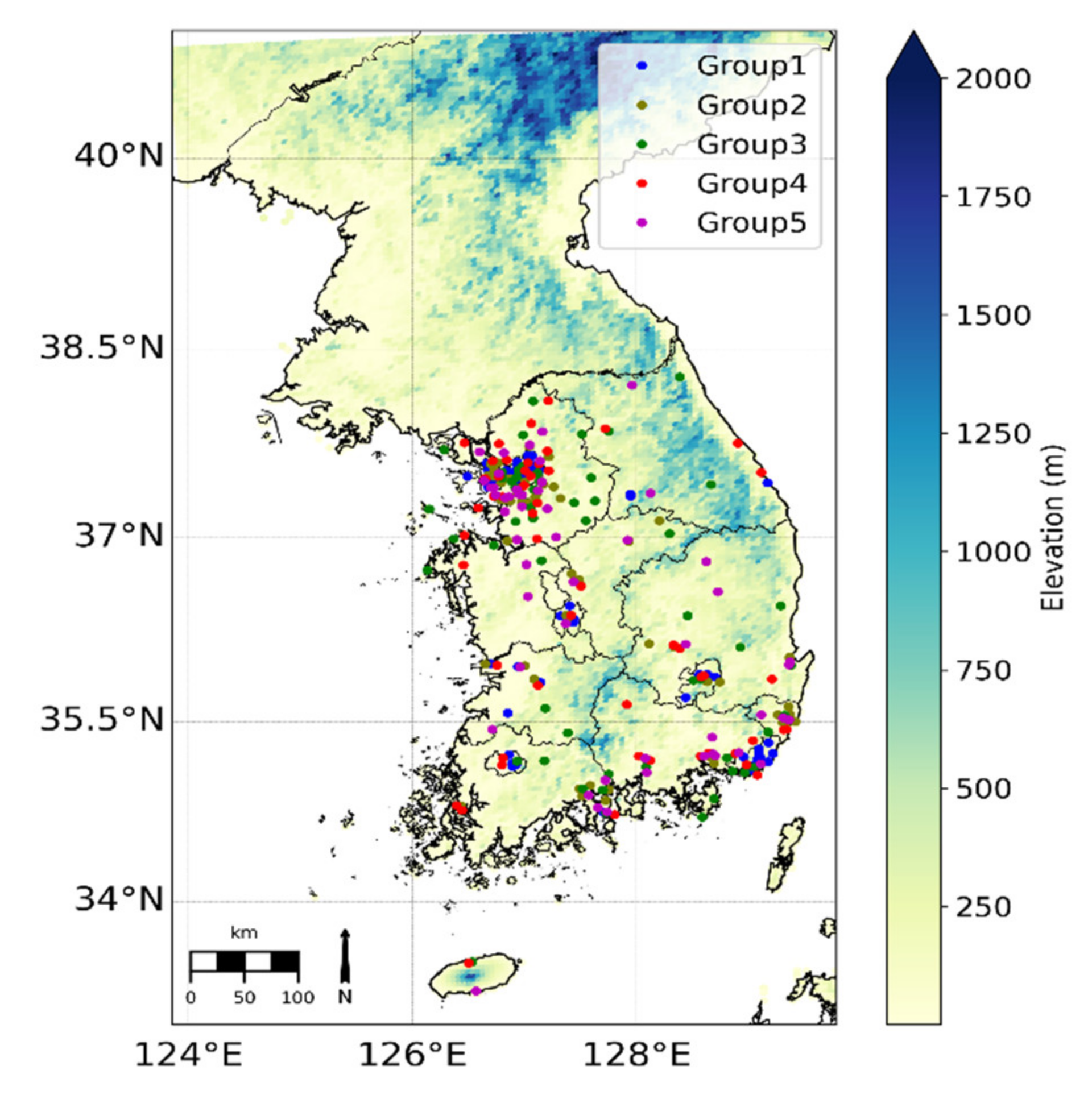
2.1. Area of Interest and Ground Measurements
2.2. Specifications of GOCI Satellite Data
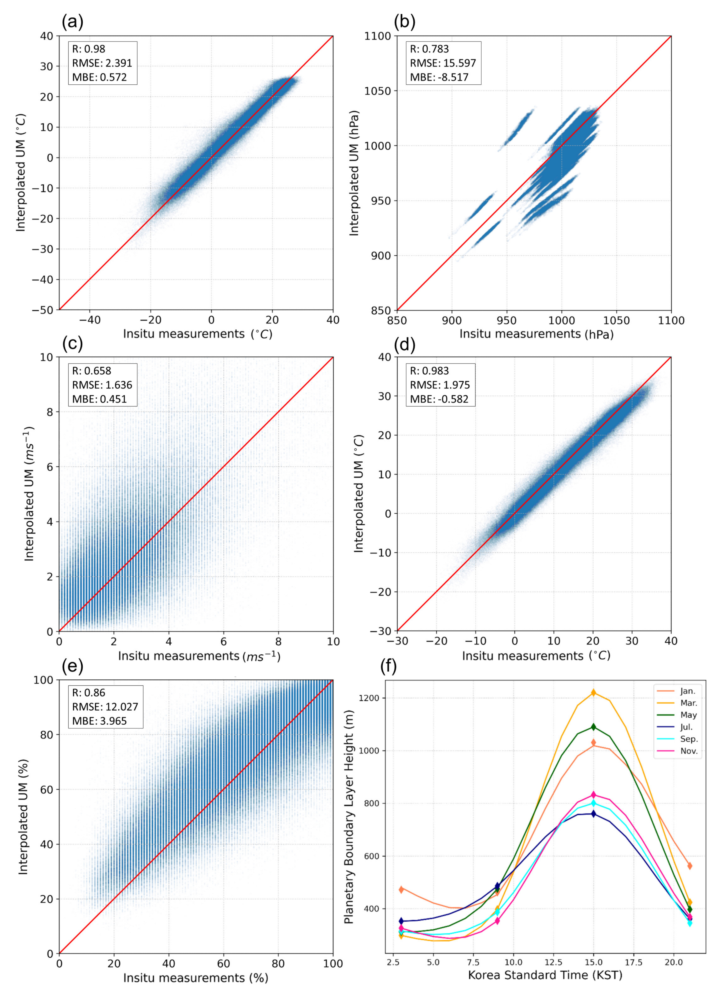
2.3. Meteorological Variables from UM Regional Data Assimilation and Prediction System (RDAPS) and Ancillary Data
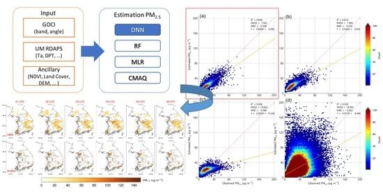
3. Methodology
3.1. Pre-Processing of Input Parameters for Training DNN
3.2. DNN Approach
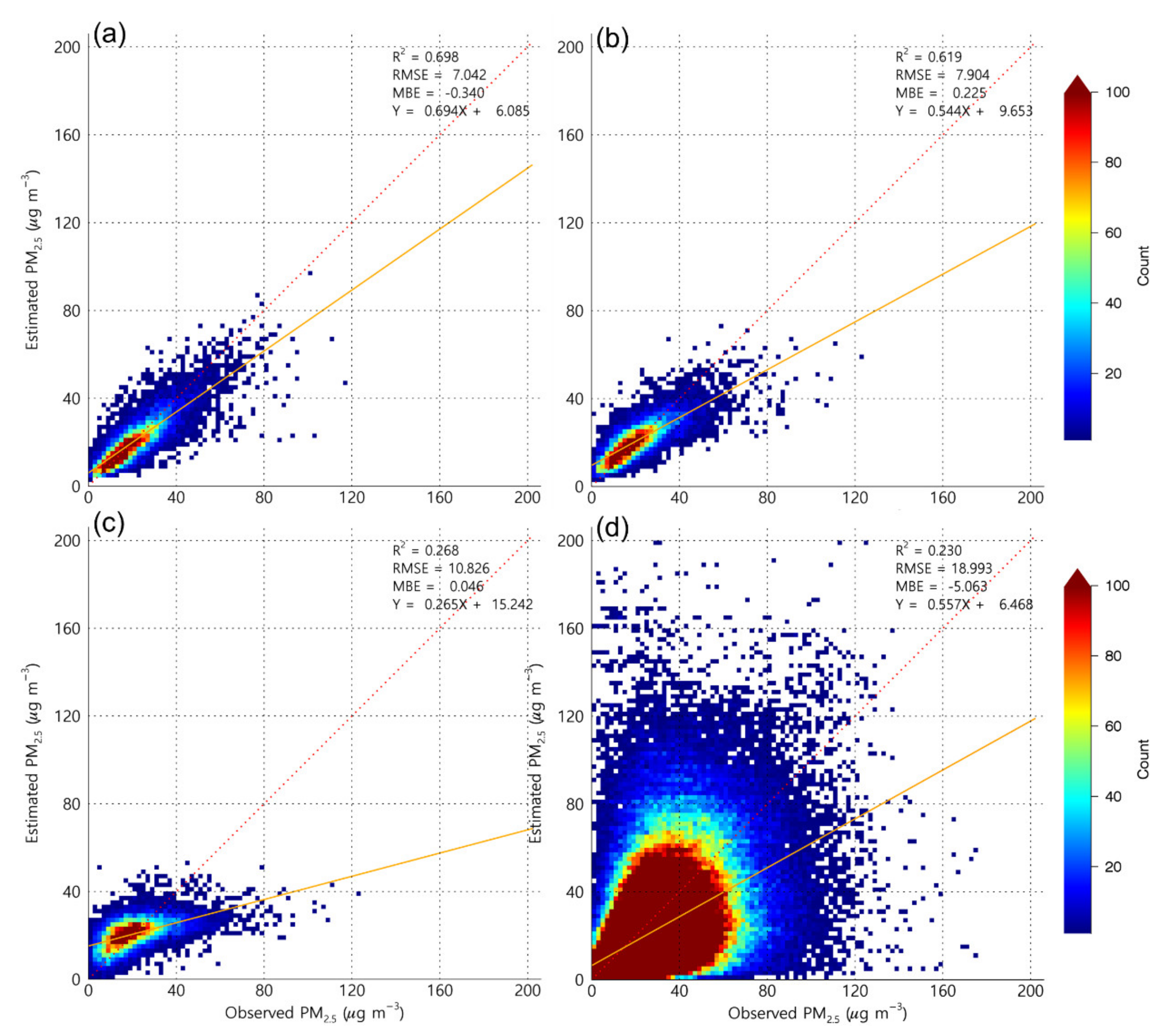
4. Results
5. Discussion
6. Conclusions
Author Contributions
Funding
Institutional Review Board Statement
Informed Consent Statement
Data Availability Statement
Acknowledgments
Conflicts of Interest
References
- Xu, J.-W.; Martin, R.V.; van Donkelaar, A.; Kim, J.; Choi, M.; Zhang, Q.; Geng, G.; Liu, Y.; Ma, Z.; Huang, L.; et al. Estimating ground-level PM2.5 in eastern China using aerosol optical depth determined from the GOCI satellite instrument. Atmos. Chem. Phys. 2015, 15, 13133–13144. [Google Scholar] [CrossRef] [Green Version]
- Guo, Y.; Tang, Q.; Gong, D.-Y.; Zhang, Z. Estimating ground-level PM2.5 concentrations in Beijing using a satellite-based geographically and temporally weighted regression model. Remote Sens. Environ. 2017, 198, 140–149. [Google Scholar] [CrossRef]
- Butt, E.W.; Turnock, S.T.; Rigby, R.; Reddington, C.L.; Yoshioka, M.; Johnson, J.S.; Regayre, L.A.; Pringle, K.J.; Mann, G.W.; Spracklen, D.V. Global and regional trends in particulate air pollution and attributable health over the past 50 years. Environ. Res. Lett. 2017, 12, 104017. [Google Scholar] [CrossRef]
- IPCC. Climate Change 2013: The Physical Science Basis. Contribution of Working Group I to the Fifth Assessment Report of the Intergovernmental Panel on Climate Change; Stocker, T.F., Qin, D., Plattner, G.-K., Tignor, M., Allen, S.K., Boschung, J., Nauels, A., Xia, Y., Bex, V., Midgley, P.M., Eds.; Cambridge University Press: Cambridge, UK; New York, NY, USA, 2013. [Google Scholar]
- Scott, C.E.; Rap, A.; Spracklen, D.V.; Forster, P.M.; Carslaw, K.S.; Mann, G.W.; Pringle, K.J.; Kivekäs, N.; Kulmala, M.; Lihavainen, H.; et al. The direct and indirect radiative effects of biogenic secondary organic aerosol. Atmos. Chem. Phys. 2014, 14, 447–470. [Google Scholar] [CrossRef] [Green Version]
- Armstrong, B.G. Effect of measurement error on epidemiological studies of environmental and occupational exposures. Occup. Environ. Med. 1998, 55, 651–656. [Google Scholar] [CrossRef] [Green Version]
- Liu, Y.; Koutrakis, P.; Kahn, R. Estimating fine particulate matter component concentrations and size distributions using satellite-retrieved fractional aerosol optical depth: Part 2-A case study. J. Air Waste Manag. Assoc. 2007, 57, 1360–1369. [Google Scholar] [CrossRef]
- Engel-Cox, J.A.; Hoff, R.M.; Haymet, A.D.J. Recommendations on the use of satellite remote-sensing data for urban air quality. J. Air Waste Manag. Assoc. 2004, 54, 1360–1371. [Google Scholar] [CrossRef]
- Xiao, Q.; Wang, Y.; Chang, H.H.; Meng, X.; Geng, G.; Lyapustin, A.; Liu, Y. Full-coverage high-resolution daily PM2.5 estimation using MAIAC AOD in the Yangtze River Delta of China. Remote Sens. Environ. 2017, 199, 437–446. [Google Scholar] [CrossRef]
- Geng, G.; Zhang, Q.; Martin, R.V.; van Donkelaar, A.; Huo, H.; Che, H.; Lin, J.; He, K. Estimating long-term PM2.5 concentrations in China using satellite-based aerosol optical depth and a chemical transport model. Remote Sens. Environ. 2015, 166, 262–270. [Google Scholar] [CrossRef]
- Gupta, P.; Christopher, S.A. Particulate matter air quality assessment using integrated surface satellite, and meteorological products: Multiple regression approach. J. Geophys. Res. 2009, 114, D14205. [Google Scholar] [CrossRef] [Green Version]
- Ma, Z.; Liu, Y.; Zhao, Q.; Liu, M.; Zhou, Y.; Bi, J. Satellite-derived high resolution PM2.5 concentrations in Yangtze River Delta Region of China using improved linear mixed effects model. Atmos. Environ. 2016, 133, 156–164. [Google Scholar] [CrossRef]
- Luo, J.; Du, P.; Samat, A.; Xia, J.; Che, M.; Xue, Z. Spatiotemporal pattern of PM2.5 concentrations in Mainland China and analysis of its influencing factors using geographically weighted regression. Sci. Rep. 2017, 7, 40607. [Google Scholar] [CrossRef] [PubMed]
- Chu, Y.; Liu, Y.; Li, X.; Liu, Z.; Lu, H.; Lu, Y.; Mao, Z.; Chen, X.; Li, N.; Ren, M.; et al. A review on predicting ground PM2.5 concentration using satellite aerosol optical depth. Atmosphere 2016, 7, 129. [Google Scholar] [CrossRef] [Green Version]
- Li, T.; Shen, H.; Yuan, Q.; Zhang, X.; Zhang, L. Estimating ground-level PM2.5 by fusing satellite and station observations: A geo-intelligent deep learning approach. Geophys. Res. Lett. 2017, 44, 11985–11993. [Google Scholar] [CrossRef] [Green Version]
- Van Donkelaar, A.; Martin, R.V.; Brauer, M.; Kahn, R.; Levy, R.; Verduzco, C.; Villeneuve, P.J. Global estimates of ambient fine particulate matter concentrations from satellite-based aerosol optical depth: Development and application. Environ. Health Perspect. 2010, 118, 847–855. [Google Scholar] [CrossRef] [Green Version]
- Yuan, Q.; Shen, H.; Li, T.; Li, Z.; Li, S.; Jiang, Y.; Xu, H.; Tan, W.; Yang, Q.; Wang, J.; et al. Deep learning in environmental remote sensing: Achievements and challenges. Remote Sens. Environ. 2020, 241, 111716. [Google Scholar] [CrossRef]
- Chen, G.; Li, S.; Knibbs, L.D.; Hamm, N.A.; Cao, W.; Li, T.; Guo, J.; Ren, H.; Abramson, M.J.; Guo, Y. A machine learning method to estimate PM2.5 concentrations across China with remote sensing, meteorological and land use information. Sci. Total Environ. 2018, 636, 52–60. [Google Scholar] [CrossRef]
- Park, S.; Shin, M.; Im, J.; Song, C.K.; Choi, M.; Kim, J.; Lee, S.; Park, R.; Kim, J.; Lee, D.W.; et al. Estimation of ground-level particulate matter concentrations through the synergistic use of satellite observations and process-based models over South Korea. Atmos. Chem. Phys. 2019, 19, 1097–1113. [Google Scholar] [CrossRef] [Green Version]
- Park, S.; Lee, J.; Im, J.; Song, C.K.; Choi, M.; Kim, J.; Lee, S.; Park, R.; Kim, S.M.; Yoon, J.; et al. Estimation of spatially continuous daytime particulate matter concentrations under all sky conditions through the synergistic use of satellite-based AOD and numerical models. Sci. Total Environ. 2020, 713, 136516. [Google Scholar] [CrossRef] [PubMed]
- Yeom, J.M.; Park, S.; Chae, T.; Kim, J.Y.; Lee, C.S. Spatial assessment of solar radiation by machine learning and deep neural network models using data provided by the COMS MI geostationary satellite: A case study in South Korea. Sensors 2019, 19, 2082. [Google Scholar] [CrossRef] [PubMed] [Green Version]
- Hinton, G.E.; Salakhutdinov, R.R. Reducing the dimensionality of data with neural networks. Science 2006, 313, 504–507. [Google Scholar] [CrossRef] [Green Version]
- Scher, S. Toward data-driven weather and climate forecasting: Approximating a simple general circulation model with deep learning. Geophys. Res. Lett. 2019, 45, 12616–12622. [Google Scholar] [CrossRef] [Green Version]
- Yeom, J.M.; Deo, R.C.; Adamowski, J.F.; Park, S.; Lee, C.S. Spatial mapping of short-term solar radiation prediction incorporating geostationary satellite images coupled with deep convolutional LSTM networks for South Korea. Environ. Res. Lett. 2020, 15, 094025. [Google Scholar] [CrossRef]
- Ong, B.T.; Sugiura, K.; Zettsu, K. Dynamically pre-trained deep recurrent neural networks using environmental monitoring data for predicting PM2.5. Neural Comput. Appl. 2016, 27, 1553–1566. [Google Scholar] [CrossRef] [Green Version]
- Sun, Y.; Zeng, Q.; Geng, B.; Lin, X.; Sude, B.; Chen, L. Deep learning architecture for estimating hourly ground-level PM2.5 using satellite remote sensing. IEEE Geosci. Remote Sens. Lett. 2019, 16, 1343–1347. [Google Scholar] [CrossRef]
- Choi, M.; Kim, J.; Lee, J.; Kim, M.; Park, Y.J.; Holben, B.; Eck, T.F.; Li, Z.; Song, C.H. GOCI Yonsei aerosol retrieval version 2 products: An improved algorithm and error analysis with uncertainty estimation from 5-year validation over East Asia. Atmos. Meas. Tech. 2018, 11, 385–408. [Google Scholar] [CrossRef] [Green Version]
- Shen, H.; Li, T.; Yuan, Q.; Zhang, L. Estimating regional ground-level PM2.5 directly from satellite top-of-atmosphere reflectance using deep belief networks. J. Geophys. Res. Atmos. 2018, 123, 13875–13886. [Google Scholar] [CrossRef] [Green Version]
- Von Hoyningen-Huene, W.; Joon, Y.; Vountas, M.; Istomina, G.; Rohen, G.; Dinter, T.; Kokhanovsky, A.A.; Burrows, J.P. Retrieval of spectral aerosol optical thickness over land using ocean color sensors MERIS and SeaWiFS. Atmos. Meas. Tech. 2011, 4, 151–171. [Google Scholar] [CrossRef] [Green Version]
- Li, X.; Cheng, G.; Lu, L. Spatial analysis of air temperature in the Qinghai-Tibet Plateau. Antarct. Alp. Res. 2005, 37, 246–252. [Google Scholar] [CrossRef]
- Li, T.; Shen, H.; Zeng, C.; Yuan, Q.; Zhang, L. Point-surface fusion of station measurements and satellite observations for mapping PM2.5 distribution in China: Methods and assessment. Atmos. Environ. 2017, 152, 477–489. [Google Scholar] [CrossRef] [Green Version]
- Peel, M.C.; Finlayson, B.L.; McMahon, T.A. Updated world map of the Köppen-Geiger climate classification. Hydrol. Earth Syst. Sci. 2007, 11, 1633–1644. [Google Scholar] [CrossRef] [Green Version]
- Byun, D.W.; Ching, J.K.S. Science Algorithms of the EPA Models-3 Community Multiscale Air Quality (CMAQ) Modeling System; EPA/600/R99/030 (NTIS PB2000-100561); U.S. Environmental Protection Agency: Washington, DC, USA, 1999. [Google Scholar]
- Skamarock, C.; Klemp, B.; Dudhia, J.; Gill, O.; Barker, D.; Duda, G.; Huang, X.; Wang, W.; Powers, G.A. Description of the Advanced Research WRF Version 3. Available online: https://doi.org/10.5065/D68S4MVH (accessed on 27 May 2008).
- Byun, D.; Schere, K.L. Review of the governing equations, computational algorithms, and other components of the Models-3 community multiscale air quality (CMAQ) modeling system. Appl. Mech. Rev. 2006, 59, 51–77. [Google Scholar] [CrossRef]
- Yeom, J.M.; Kim, H.O. Comparison of NDVIs from GOCI and MODIS data towards improved assessment of crop temporal dynamics in the case of paddy rice. Remote Sens. 2015, 7, 11326–11343. [Google Scholar] [CrossRef] [Green Version]
- Hsu, N.C.; Jeong, M.J.; Bettenhausen, C.; Sayer, A.M.; Hansell, R.; Seftor, C.S.; Huang, J.; Tsay, S.C. Enhanced Deep Blue aerosol retrieval algorithm: The second generation. J. Geophys. Res. Atmos. 2013, 118, 9296–9315. [Google Scholar] [CrossRef]
- Pinty, B.; Verstraete, M.M. GEMI: A non-linear index to monitor global vegetation from satellites. Vegetation 1992, 101, 15–20. [Google Scholar] [CrossRef]
- Park, S.; Lee, D.U.; Seo, J.W. Operational wind wave prediction system at KMA. Mar. Geod. 2009, 32, 133–150. [Google Scholar] [CrossRef]
- Mahdian, M.H.; Bandarabady, S.R.; Sokouti, R.; Banis, Y.N. Appraisal of the geostatistical methods to estimate monthly and annual temperature. J. Appl. Sci. 2009, 9, 128–134. [Google Scholar] [CrossRef]
- Nguyen, X.T.; Nguyen, B.T.; Do, K.P.; Bui, Q.H.; Nguyen, T.N.T.; Vuong, V.Q.; Le, T.H. Spatial interpolation of meteorological variables in Vietnam using the Kriging method. J. Inf. Process. Syst. 2015, 11, 134–147. [Google Scholar] [CrossRef] [Green Version]
- Chu, Y.; Li, J.; Li, C.; Tan, W.; Su, T.; Li, J. Seasonal and diurnal variability of planetary boundary layer height in Beijing: Intercomparison between MPL and WRF results. Atmos. Res. 2019, 227, 1–13. [Google Scholar] [CrossRef]
- Xie, M.; Zhu, K.; Wang, T.; Feng, W.; Gao, D.; Li, M.; Li, S.; Zhuang, B.; Han, Y.; Chen, P.; et al. Changes in regional meteorology induced by anthropogenic heat and their impacts on air quality in South China. Atmos. Chem. Phys. 2016, 16, 15011–15031. [Google Scholar] [CrossRef] [Green Version]
- Chang, Y.; Zou, Z.; Deng, C.; Huang, K.; Collett, J.L.; Lin, J.; Zhuang, G. The importance of vehicle emissions as a source of atmospheric ammonia in the megacity of Shanghai. Atmos. Chem. Phys. 2016, 16, 3577–3594. [Google Scholar] [CrossRef] [Green Version]
- Zhang, D.; Zhang, W.; Huang, W.; Hong, Z.; Meng, L. Upscaling of surface soil moisture using a deep learning model with VIIRS RDR. ISPRS Int. J. Geo. Inf. 2017, 6, 130. [Google Scholar] [CrossRef]
- Breiman, L. Random forests. Mach. Learn. 2001, 45, 5–32. [Google Scholar] [CrossRef] [Green Version]
- Geng, G.; Meng, X.; He, K.; Liu, Y. Random forest models for PM2.5 speciation concentrations using MISR fractional AODs. Environ. Res. Lett. 2020, 15, 034056. [Google Scholar] [CrossRef]
- Zang, L.; Mao, F.; Guo, J.; Gong, W.; Wang, W.; Pan, Z. Estimating hourly PM1 concentrations from Himawari-8 aerosol optical depth in China. Environ. Pollut. 2018, 241, 654–663. [Google Scholar] [CrossRef] [PubMed]


| Parameter | Configuration | ||||
|---|---|---|---|---|---|
| Number of hidden nodes | 64 | 128 | 256 | 512 | 1024 |
| Number of hidden layers | 3–4 | 4–6 | 4–6 | 6–8 | 6–8 |
| L1 regularization | False, 0.01, 0.001, and 0.0001 | ||||
| L2 regularization | False, 0.01, 0.001, and 0.0001 | ||||
| Activation function | ReLu, Leaky ReLu, and exponential linear unit (ELU) | ||||
| Optimization | Adam and root mean square propagation (RMSProp) | ||||
| Learning rate | 0.05, 0.001, and 0.005 | ||||
| Dropout rate | 0.1, 0.2, and 0.3 | ||||
| Method | RMSE | MBE | R2 |
|---|---|---|---|
| DNN | 9.166 | 0.293 | 0.49 |
| RF | 9.342 | 0.337 | 0.474 |
| MLR | 11.133 | −0.0428 | 0.251 |
Publisher’s Note: MDPI stays neutral with regard to jurisdictional claims in published maps and institutional affiliations. |
© 2021 by the authors. Licensee MDPI, Basel, Switzerland. This article is an open access article distributed under the terms and conditions of the Creative Commons Attribution (CC BY) license (https://creativecommons.org/licenses/by/4.0/).
Share and Cite
Lee, C.; Lee, K.; Kim, S.; Yu, J.; Jeong, S.; Yeom, J. Hourly Ground-Level PM2.5 Estimation Using Geostationary Satellite and Reanalysis Data via Deep Learning. Remote Sens. 2021, 13, 2121. https://doi.org/10.3390/rs13112121
Lee C, Lee K, Kim S, Yu J, Jeong S, Yeom J. Hourly Ground-Level PM2.5 Estimation Using Geostationary Satellite and Reanalysis Data via Deep Learning. Remote Sensing. 2021; 13(11):2121. https://doi.org/10.3390/rs13112121
Chicago/Turabian StyleLee, Changsuk, Kyunghwa Lee, Sangmin Kim, Jinhyeok Yu, Seungtaek Jeong, and Jongmin Yeom. 2021. "Hourly Ground-Level PM2.5 Estimation Using Geostationary Satellite and Reanalysis Data via Deep Learning" Remote Sensing 13, no. 11: 2121. https://doi.org/10.3390/rs13112121