Technical Note

Salt Marsh Elevation Limit Determined after Subsidence from Hydrologic Change and Hydrocarbon Extraction

1
Department of Oceanography and Coastal Sciences, Louisiana State University, Baton Rouge, LA 70803, USA
2
School of Geography and the Environment, University of Oxford, Oxford OX1 3QY, UK
*
Author to whom correspondence should be addressed.
Remote Sens. 2021, 13(1), 49; https://doi.org/10.3390/rs13010049
Submission received: 25 October 2020 / Revised: 18 December 2020 / Accepted: 20 December 2020 / Published: 25 December 2020
(This article belongs to the Special Issue Satellite and Ground Remote Sensing for Wetland Environments)

Abstract

:
Levee construction aboveground and hydrocarbon removal from belowground in coastal wetlands can create hydrologic changes that increase plant stress through flooding. But the significance of the subsidence they cause individually or in combination is contested. This study untangled them to demonstrate elevational limits of salt marshes by studying dredged and natural waterways in two salt marshes in Louisiana, USA. The areas had a homogenous plant cover before drilling for oil and gas extraction peaked in the 1960s, and now are a mixed network of natural waterways and dredged canals used to drill wells with an average drill date of 1965.8 ± 2.7 (µ ± 1 SEM; n = 18) and well depth of 4661.0 m ± 56.6 (µ ± 1 SEM; n = 18). Aerial imagery was used to document how canals widened to become 2 to 4 times larger than their original construction width at the high production site and 50% larger at the low production site, whereas increases at the nearby natural channels were much less. Light detection and ranging (LIDAR) measurements at the high production site from 2002 showed that the marsh surface near wells subsided by 34 cm compared to undredged sites. Elevation in marshes at producing and dry wells were equal at the low production site, but high production well locations were even lower than at dry wells. An elevation vs. percent open water curve developed from these data overlapped with an independent analysis of a brackish marsh. A relative subsidence rate between 7.4 to 10.4 mm y−1 transformed these salt marshes to an open water habitat within a few decades. The local creation of accommodation space through hydrocarbon removal and leveed wetlands is a parsimonious explanation for the spatial and temporal land loss rates on this deltaic coast over the last 80 years of oil and gas exploration. Substantial losses from the accelerating rates of sea level rise are indicated to occur before 2050.

Graphical Abstract

1. Introduction

Modifying flooding with levees in the surface layers and hydrocarbon removal from thousands of meters below the surface are significant human interventions in coastal wetlands. Both agents are demonstrably influential where the other is absent, and they exist together in coastal zones including in Nigeria and Venezuela [1,2], and notably in Louisiana, USA, where both are seen as potential causes of why 25% (4833 km2) of the coastal wetlands existing in 1932 converted to open water by 2016 [3]. The reasons for this land loss are partially related to the direct removal of wetlands by dredging but, more importantly, how wetlands interact with the changed water level and flooding frequencies. Changes in flooding depths are dependent on both subsidence within surface soils and deep strata, and on the sea level. Quantifying the relationship between vegetative cover and flooding has broad implications for the future of wetlands as sea level rise (SLR) accelerates and flooding increases.
The removal of gas, oil, and water from far below the wetland surface can cause significant subsidence which may increase plant flooding, distress, and then loss. The subsidence rates can be many times higher than the 5.9 mm y−1 SLR referenced to tide gage measurements on relic coral substrates from 1999 to 2019 in the Gulf of Mexico at Key West, Florida or the 10 mm y−1 SLR at Cedar Key, Florida (https://www.psmsl.org/data/obtaining/stations/188.php). For example, the subsidence rates were 1 mm d−1 in two Californian oilfields (not in wetlands) [4], up to 200 mm y−1 in El Polvorin, Lagunillas, Venezuela (a poldered coastal lagoon) [1], and 250 mm y−1 at aquaculture facilities located on a 160-year-old part of the Yellow River delta in China [5]. Xu et al. [6] measured 150 mm of subsidence in only 3 months in the Lost Hills oil fields, Southern California and suggested that the deformation there could be used to measure hydrocarbon recovery volumes. The subsidence in an oil field usually creates the shape of a bowl centered over the drilling site when viewed laterally and may continue to extend beyond the extraction pool after field closure. For example, land subsidence in the 23,470 km2 Dongguo Marsh Field in China (1.6 km deep; no fault zones) was >100 mm y−1 and extended out 5000 m or more from the extraction center [7]. Lateral slip zones may be stimulated post-abandonment and subsidence may increase in more distal areas as fluid reservoirs migrate towards the proximal reservoirs with the recently reduced pressures [8,9]. The expression of subsidence at the soil surface, therefore, may be nonlinear with time [10] and continue for more than a decade after hydrocarbon extraction ends [11]. Porewater pressure usually decreases with oil or gas withdrawal (e.g., by 20 MPa in the subsiding oil fields of California [12]), but not always. High-porosity soils in Mexico City, for example, subsided 9 m, but the pore pressure declined only 0.7 MPa [12].
Several authors concluded decades ago that subsidence from hydrocarbon production was an insignificant influence on Louisiana’s coastal wetland loss because the recovery sites were too deep and the subsidence rates too small to have an effect [13,14]. Others have since described the spatial and temporal coincidence of hydrocarbon recovery and wetland loss around individual oil fields and concluded that wetland loss within oil and gas fields in the entire Louisiana deltaic plain was primarily driven by subsidence induced by local hydrocarbon extraction [10,15,16,17,18,19].
An alternative explanation for these wetland losses in Louisiana is related to the dredging of canals used to bring the equipment and people to drill and maintain wells. The dredged material is deposited in a mostly continuous levee alongside the canal called a “spoil bank”. The canal/spoil bank complex becomes a wetland plant stressor independent of whatever subsidence results from hydrocarbon recovery because of the spoil bank height, length, and soil density. The initial height of a spoil bank on the Louisiana coast is multiples of the tidal range, and the length of spoil banks is enough to cross Louisiana’s coastal zone 78 times from east to west [20]. The height of the spoil bank blocks water entering and leaving aboveground during normal tidal fluctuations and the sediment-rich spoil bank becomes a barrier for belowground flows because its mass is denser than the organic surface soils of the marsh it was deposited on. This above- and belowground hydrologic obstruction creates one-third fewer drying cycles in the marsh that are each 40% longer, and 75% fewer wetting cycles which are each 5 times longer on the marsh [21], causing a decrease in the marsh surface elevation that declines with age [22]. The increased wetland inundation changes the amount of the belowground plant biomass which is necessary for vertical accretion and erosion resistance [22] and creates the potential for toxic conditions such as sulfide accumulation [23,24]. The longer drying cycles lead to soil matter oxidation—and organic carbon is the main material contributing to vertical growth and soil strength in salt marshes [25]. The effect of introducing spoil banks may be quick. Wetlands in Terrebonne Parish, for example, went from 15% to 85% open water within two years after a canal was dredged across it [26]. A coastwide view is that the rise and fall of wetland loss in Louisiana’s deltaic plain coincides with the rise and fall of canal growth, and that the spatial density of canals is directly related to wetland loss outside of the immediate area of the river delta terminus [20].
Enhanced subsidence and altered hydrologic patterns, therefore, were created simultaneously in time and space over the last 100 years, making quantification of their relative influence on wetland loss problematic for a natural resource with an economic valuation that is higher than most habitat types [27]. One useful clue is that bottom hole pressures in producing reservoirs may not have any effect on pressures in adjacent wells [8,10]. The potential significance of this observation is that determining subsidence rates around individual wells may be helpful to separate out the effects of hydrocarbon extraction from the effects of spoil banks at the salt marsh surface. We used this observation to address this quandary about the relative causes and to demonstrate a tipping point for wetland conversion to open water as the rate of SLR accelerates, which is a widely identified future cause for marsh loss in the area [28].
Here we tested the hypothesis that the spoil bank/canal complex by itself, and in combination with hydrocarbon recovery, has a measurable impact on salt marsh elevation in coastal Louisiana. We used light detection and ranging (LIDAR)-based digital elevation model (DEM) data to measure the relative elevations along transects crossing natural channels and at dredged waterways built to recover hydrocarbons, and to discriminate between the amount of subsidence around dry wells, producing wells and natural waterways. We tested if there was a significant correlation between the marsh elevation loss and hydrocarbons produced, and if canals and natural channels widened at different rates from 1960 to 2016. We then used these measurements to determine if a coastwide loss of salt marshes is imminent.

2. Materials and Methods
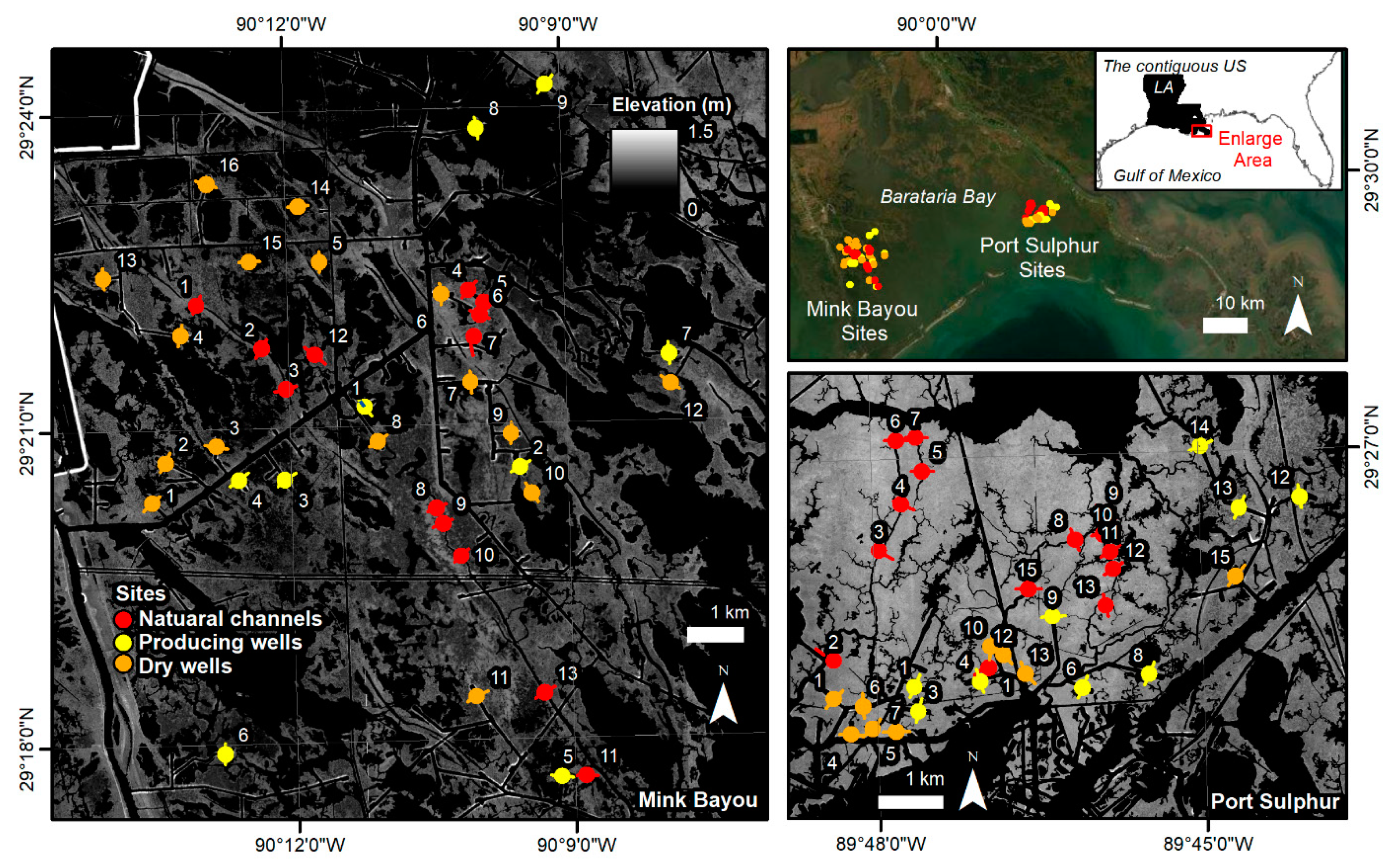
2.1. Study Areas

The two study areas are on the east and west side of Barataria Bay, LA, USA (Figure 1). The 30-cm tidal range is dominated by meteorological rather than astronomical forcing that distinguishes the Gulf of Mexico (GOM) estuaries from other coastal US estuaries [29]. The Port Sulphur, LA area is bordered on the north by Bay San Bois and Bayou Dulac, on the west by Bay Batiste, and by Lake Grande Ecaille to the south. It was a nearly continuous wetland plant cover on United States Geological Survey (USGS) maps in 1935 (7.5-min quadrangle map; Bay Batiste, LA) and 1945 (15.0-min quadrangle map; Fort Livingston, LA) and is dominated by salt marsh plants (Spartina alterniflora, S. patens, and Juncus roemerianus). The second area is within the Mink Bayou USGS quadrangle map (7.5-min; 1:24,000 scale). It was covered with the same emergent vegetation in both the 1946 and 1954 USGS maps (Mink Bayou 7.5-min quadrangle) and is bordered on the west by Bayou Lafourche, has channel bifurcations running north to south through it, and is populated by several lakes. Field observations indicate that the vegetation has not changed categorization in four categories since the mapping analysis within a 1949 report on muskrats [30]. A time-series of the development of the dredged channels at both sites from 1930s to 2001 is in the Supplemental Materials (Figures S1 and S2).

2.2. Hydrocarbon Extraction

The study area today contains many waterways dredged to construct hydrocarbon extraction wells. The wells can be “dry wells”, which were drilled but yielded neither oil or gas, or “production wells”, which were dredged and produced oil, gas, or both oil and gas. We selected 18 production wells (9 at each area) and 25 dry wells (9 in Port Sulphur and 16 in Mink Bayou) and matched them with 27 nearby natural waterways (14 in Port Sulphur and 12 in Mink Bayou). The drill dates and well depths are from the Louisiana Department of Natural Resources permitting records (http://sonris-www.dnr.state.la.us/gis/). The locations of the selected wells and their permit number are in Supplementary File S1 and Tables S1 and S2. The average drilling start dates and standard errors for all dredged canals at Port Sulphur and Mink Bayou were 1965.77 ± 2.69 y and 1966.6 ± 1.89, respectively. The average depths of the producing well were 4661 ± 57 m and 4066 ± 123 m at Port Sulphur and Mink Bayou, respectively. In order to sample similar hydrologic features, all well locations sampled: (1) Had marsh on both sides of the pre-dredged quadrangle map, (2) were at least 300 m from the nearest canal or waterway, (3) were not crossed with a natural channel or levee, and (4) were “dead” end canals not situated within an oil field. Measurements were made about 50 m from the enlarged terminal end of the canal (also known as “keyhole”) with the wellhead and where the boats’ servicing facilities turn around.

2.3. LIDAR Measurements

The elevations of adjoining salt marshes of the waterways were measured using LIDAR (light detection and ranging) imagery with a 5 × 5 m spatial resolution (vertical datum NAVD88, horizontal datum NAD 83). The LIDAR imagery is from the DEM produced by the Louisiana Federal Emergency Management Agency (FEMA) Project and distributed by “Atlas: The Louisiana Statewide GIS” at the Louisiana State University CADGIS Research Laboratory, Baton Rouge, LA (http://atlas.lsu.edu). The DEM were derived from LIDAR measurements performed in 2002 and are in the USGS (non-SDTS) DEM format. The Root Mean Square Error of the data of all major land cover types (i.e., low grass, high grass, brush lands, forested, and urban [31]) was 11.52 cm [32]. The error may have been larger in the marsh area due to dense short vegetation and standing water [33]. However, because this study only compared elevations at different sites, the effect of such an error on our assessment was likely to be negligible. The original source of the LIDAR data is in File S1. Downloading and analysis of LIDAR data were done without a priori knowledge of their site categorization.
Transects of 150-m long were on both sides of the land–water edge of 70 waterways, and the elevations were measured in 5-m increments. The transects were perpendicular to the land–water interface and extended over the natural levee or spoil bank and into the salt marsh, resulting in two transects for each waterway. The transects in dredged waterways were about 50 m outside of the keyhole with the drillhole because possible complications to LIDAR signals by service platforms and storage facilities. The water surface was defined as 0.08 m in the raw data, which was subtracted from all the elevation data. The elevations along transects extending out from both sides of watercourses were averaged for each of the three site categories (natural, dry wells, or producing wells) and the ±1 standard error of the mean (SEM) calculated using Prism (Prism 8.4.2 (464) software© 2020 GraphPad Software, Inc., La Jolla, CA, USA).
For each area, an ANOVA was performed along with a Brown–Forsythe test of equal variance, and a Kruskal–Wallis test for non-parametric distributions to test if the elevation in 2002 was different among waterway categories: (1) at each distance away from the water’s edge, (2) for all sampling locations, and (3) at locations between 75 to 125 m from the water’s edge. Violin plots of the elevation data were constructed to visually describe the width of the distribution of points in proportion to the number of points at that Y value.

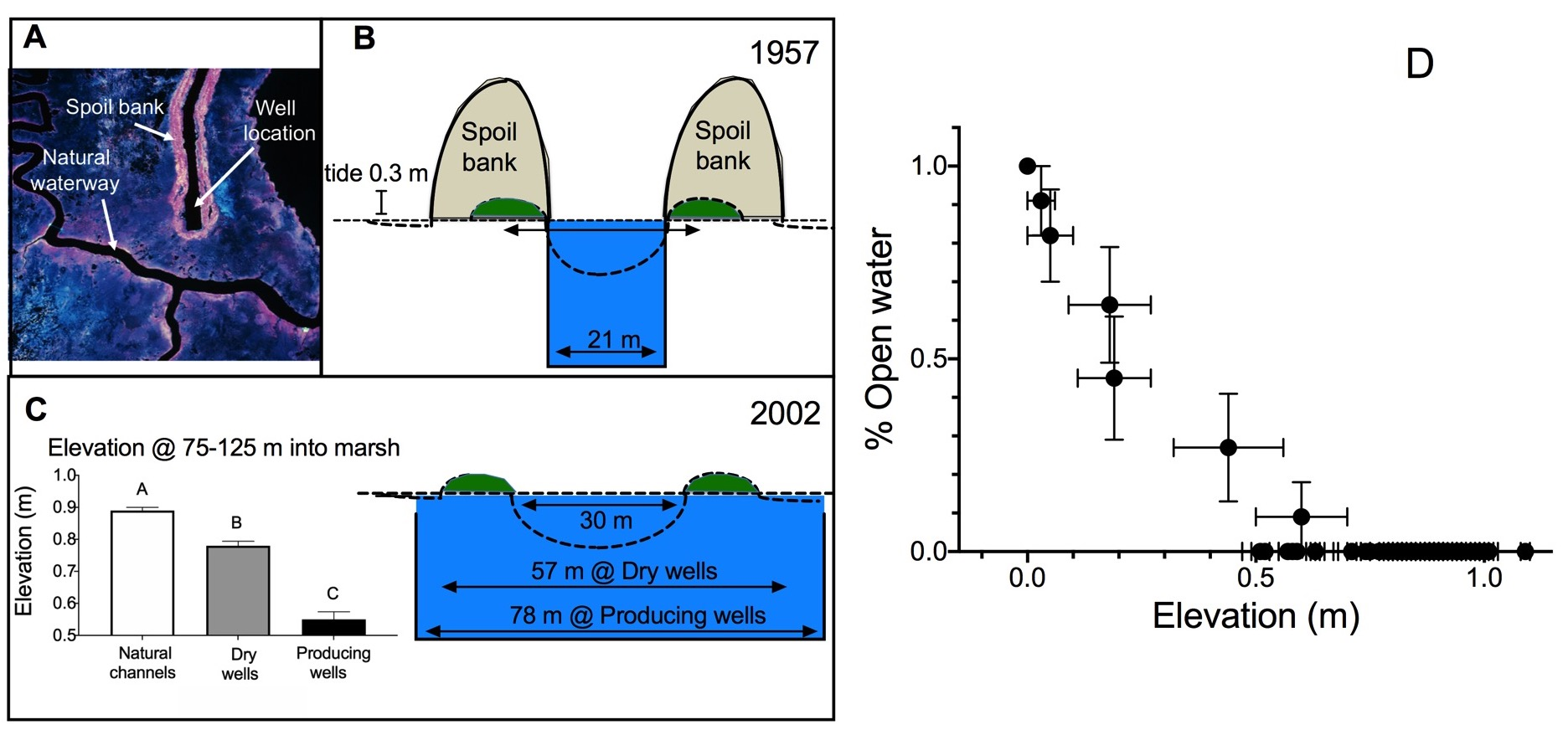
2.4. Mid-Transect Open Water

We estimated the amount of open water and marsh elevation in order to determine elevation limits for the emergent plants. The LIDAR measurements indicated that there was an elevation depression at >50 to 125 m distance along both transects, which became higher at the far end away from the dredged channel of the Port Sulphur transects. We measured the elevation of this lowest section by calculating the elevation for each 5-m interval from 75 to 125 m (n = 11) at each transect and then compared the elevations to the percent open water at that distance interval for each sample area. The mean ± 1 SEM was calculated for each transect on both sides of the waterway (Port Sulfur/Mink Bayou) for natural channels (n = 28/26), at producing wells (n = 18/18), and at dry wells (n = 18/18) for a total of 140 discrete measurements. The data were then fit to a log:linear curve where elevation (X) was linear and the percent open water (Y) was transformed to plot log values on a linear scale. The results were graphically compared to Stagg et al.’s [34] study of brackish marsh elevation and fragmentation in an S. patens coastal marsh located in the Chenier Plain of Texas along the Northern Gulf of Mexico. An ANOVA using Tukey’s multiple comparison tested if there were differences in elevation among the three site categories from 75 to 125 m from the water’s edge for all individual 5-m samplings in this distance range. An additional analysis used the measuring tool in Google Earth to estimate the open water in 2019 in the 50- to 125-m transect for only those plots that had zero percent open water in the LIDAR data set.

2.5. Subsidence and Hydrocarbon Production
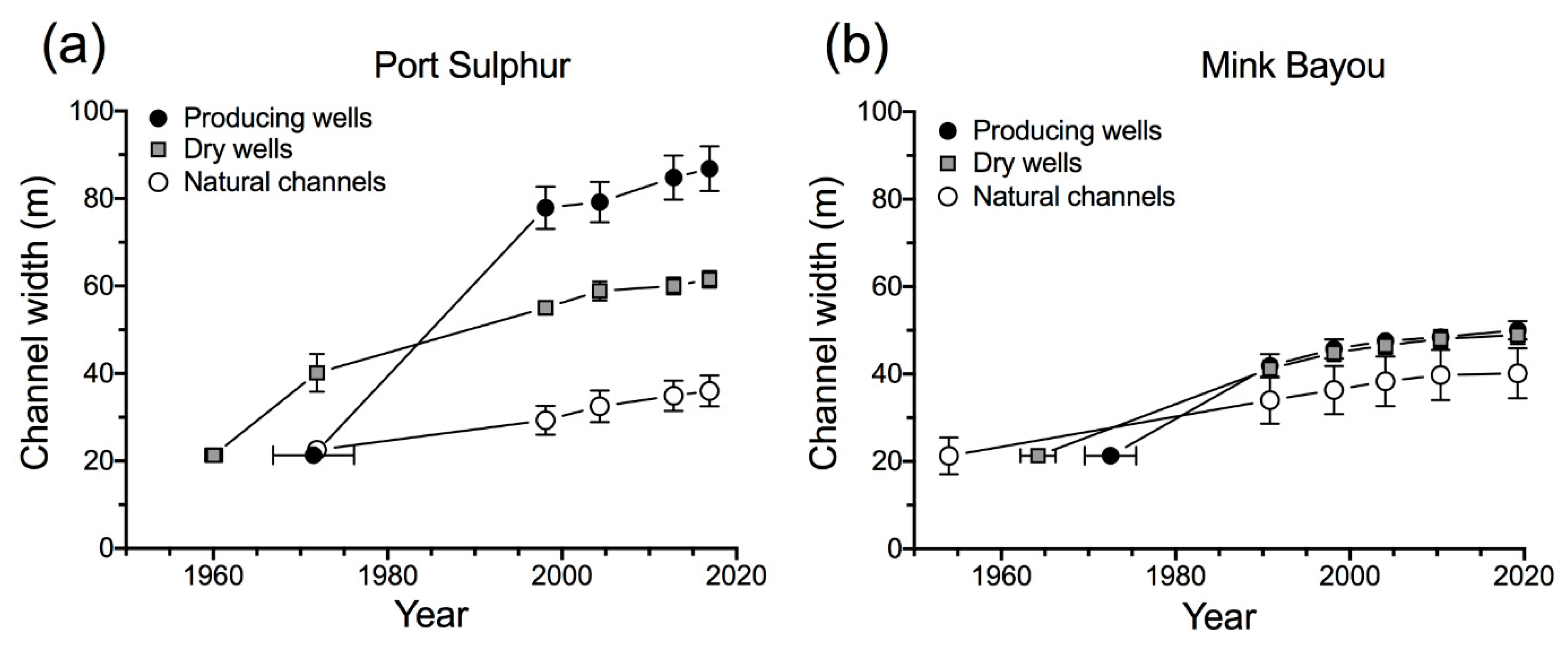
The elevation at 75 to 125 m distance (n = 11) along both sides of each transect was averaged for all production well locations. The volumetric recovery of hydrocarbons at each site up to the time of the LIDAR data collection was compared to the elevation in this 75- to 125-m distance range, and a simple linear regression analysis was made that included the average elevation for the non-dredged sites (0 production, 0.78 m elevation). Only the data from Port Sulphur had a line fitted to the data because of the relatively low production volume at Mink Bayou.

2.6. Channel Width

Waterway widths were measured across the transect line on the 1973 United States Geological Survey maps (7.5-min quadrangle map; Port Sulphur, LA and Bay Batiste, LA; (21 November 1971 imagery) (1954 Mink Bayou quadrangle map; 1952 and 1956 imagery) and Google Earth Pro (version 7.3.2.5776) using its measuring tool for 1998, 2004, 2012, 2016, and 2019 (when available).

3. Results

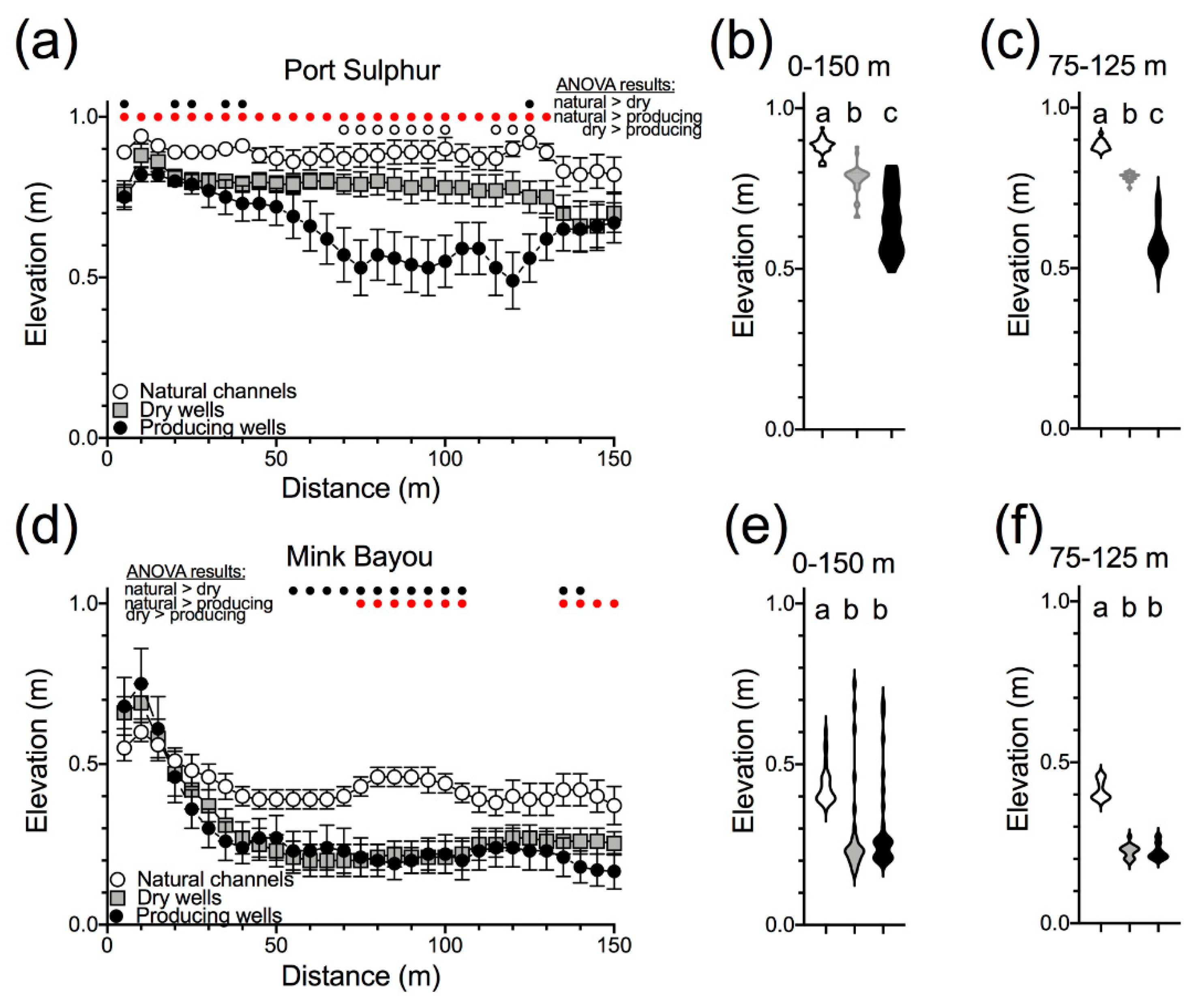
3.1. Elevation and Canal Widening

The elevation at Port Sulphur for all 5-m data points going away from the water’s edge up to 150 m into the salt marsh ranged from 0.49 to 0.89 m and overall was highest in marshes alongside natural channels, lower in salt marshes with dry wells, and lowest in sites with producing wells (Figure 2a–c). The difference in marsh elevation between sites with natural channels and dry wells was about 38% of the difference in elevation between marshes at natural channels and producing wells. Salt marshes at the natural channels had higher elevations than in salt marshes with dry wells at 6 of the 30 distance intervals. Five of the six were within 40 m of the water’s edge, and the sixth was at the end of the transect. The marsh elevation alongside natural channels was higher at 26 of 30 intervals for salt marshes with producing wells. Salt marshes with dry wells had higher elevations than salt marshes with producing wells at 10 of 30 intervals, and these 10 locations were at the mid-range of the transect.
The average elevation for Port Sulphur data from the 75- to 125-m zone (µ ± 1 SEM) of the marshes with natural channels was 0.89 ± 0.01 m (n = 308), 0.78 ± 0.014 m (n = 198) at the sites with dry wells, and 0.55 ± 0.024 m (n = 198) at sites with producing wells (Figure 2c). The ANOVA results demonstrate that these elevations were significantly different from each other (p < 0.001). The changes in salt marsh elevation equaled 0.11 m for the dry well sites and 0.34 m at the sites with producing wells, respectively, relative to salt marsh elevation at sites with natural channels. In comparison to the natural marshes, the average annual elevation decline from construction to the time of LIDAR measurements was 3.0- and 9.4-mm y−1 at sites with dry and producing wells, respectively.
The maximum and minimum elevation at Mink Bayou for all 5-m data points ranged from −0.06 to 1.35 m and was highest in marshes alongside dredged channels, and lowest in salt marshes with either dry or producing wells (Figure 2e). The average elevations along an individual transect at dry and producing wells were not different from each other (Figure 2e,f), and were 66% of the elevation for marshes at natural channels. Salt marshes at the natural channels had higher elevations than in salt marshes with dry or producing wells at 13 and 11 intervals, respectively, of the 30 distance intervals (Figure 2d).
The original throat of canals was 21.3 m wide and 4.7 m deep [35], and the canals widened to more than twice that by the time the LIDAR data were collected in 2002 (Figure 3). A simple linear regression of channel width yielded estimates of widening from 1990 to 2019 at Mink Bayou of 0.23, 0.26, and 0.27 m y−1 at natural, dry, and producing sites, respectively, and 0.3, 0.67, and 1.09 m y−1 at the Port Sulphur natural, dry, and producing sites, respectively. These numbers mean that the Port Sulphur area canal widths for production sites were at least 50% larger (+20 m) than at the dry well sites by 2016, and 3.5 times larger than the original width. The changes by the time the LIDAR measurements were made (2002) also means that the first data point at 5 m in Figure 1 is at the salt marsh side behind the original levee; in other words, there was erosion of the original spoil bank and some marsh by 2002. That the 2002 data point was at a lower elevation than at the 5-m distance in salt marshes next to dredged waterways could have been from the loss of the surficial sediment through erosion, organic matter oxidation, or reduced accumulation relative to the marshes alongside natural channels. A possible explanation is that the dredged material that was originally piled up as a spoil bank and from the eroding canal edge was a source of sediment to the marsh within 70 m of the water’s edge. A canal widening of 20 m to the same depth of the original canal would have nine times more volume than the cumulative difference in marsh elevation at the sites with dry and producing wells. This localized sediment source likely compensated for the subsidence from mineral recovery close to the drilling site and raised the elevation enough to distort the surface depression so that a cross section was raised at the drilling point and was not completely bowl-shaped at the water’s edge (Figure 2a). The slower widening rate at Mink Bayou canals did not deconstruct the spoil bank, and so the height measurements at the beginning of the transect were visually higher than in the natural marsh than in dredged marshes, although the statistically defined difference was not apparent (Figure 2).

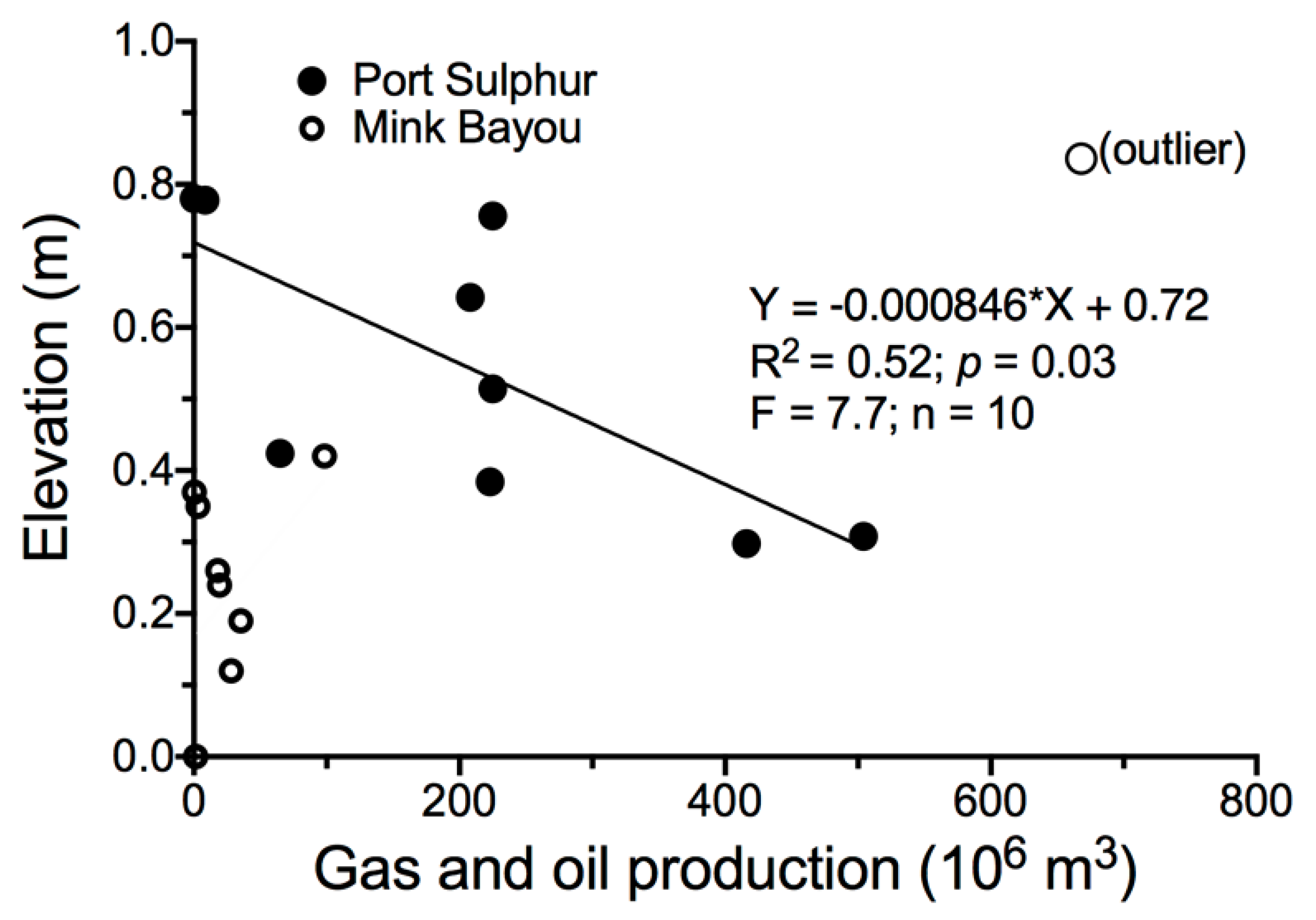
3.2. Subsidence and Hydrocarbon Production

The elevation in salt marshes 75 to 150 m from the canals with oil and gas production at Port Sulphur marshes is inversely related to the production of hydrocarbons (Figure 4). The oil and gas production for wells at the Port Sulphur study area ranged from 9 to 668 × 106 m3. The variation in the volume of hydrocarbon extracted explains about half of the elevation differences (R2 = 0.52). The one outlier is for a canal created in 1957 that had the highest hydrocarbon recovery amount. The oil and gas production for individual wells at the Mink Bayou marshes was small relative to those at Port Sulphur marshes, and ranged from 0.4 to 98 × 106 m3 and was not correlated to elevation differences.

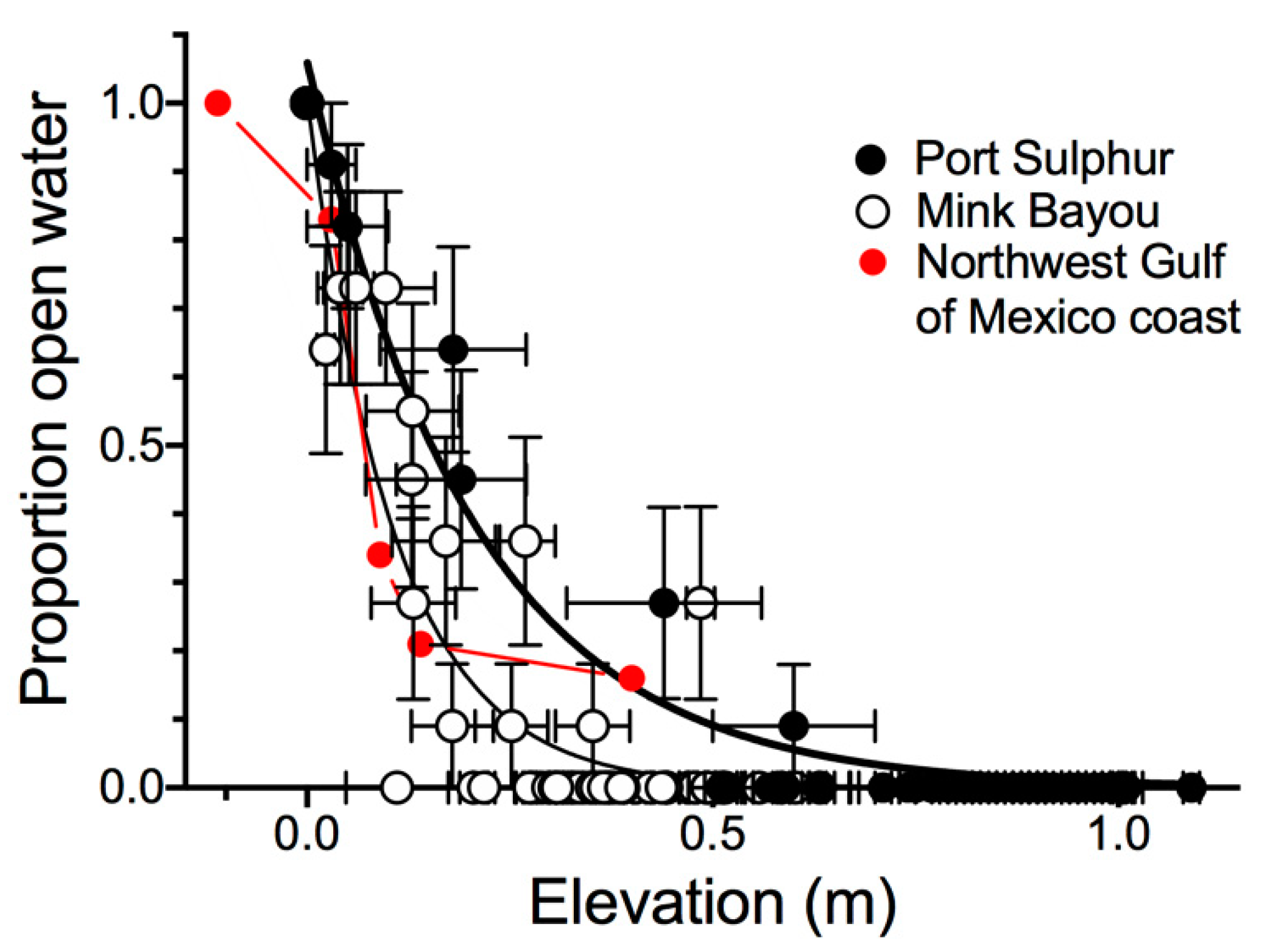
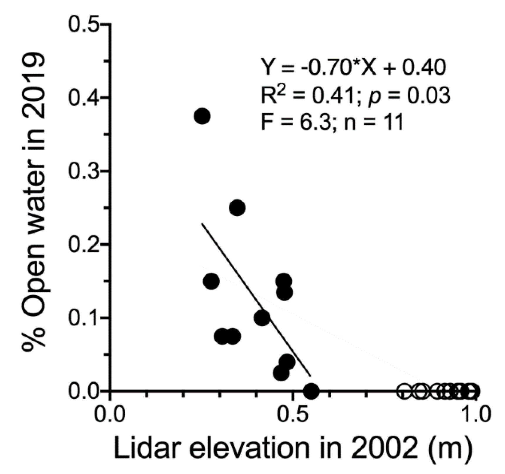
3.3. Mid-Transect Open Water and Elevation

The percent of open water (ponding) increased as the elevation of the salt marsh decreased at the two locations, but at different rates (Figure 5). The logarithmic relationship between the log10 percent ponding and elevation had an R2 = 0.72 at Port Sulphur and 0.77 at Mink Bayou. Those curve fits have a “break-point” between 0.4 to 0.6 m, which is where open water starts to develop as the salt marsh begins fragmenting. The curves for these two salt marshes overlap the elevation vs. percent open water curve for an S. patens marsh in a coastal marsh in the northwest coast of the Gulf of Mexico which was developed using aerial imagery and a fragmentation index [34].
The percent open water in the entire 75- to 125-m zone (µ ± 1 SEM) of Port Sulphur marshes with natural channels was 2.3 ± 0.01% (n = 308), 4.0 ± 0.014% (n = 198) at sites with dry wells, and 19.7 ± 2.8% (n = 198) at sites with producing wells. The percent of open water between 75 and 125 m away from the salt marsh/water interface was, therefore, 5 times higher at production well locations than at dredged locations that had dry wells, and 8.6 times higher than at natural channels. The equivalent comparison at Mink Bayou was that the average percent open water in marshes at 75 to 125 m along the transects with dry and producing wells were both 8 times higher than in the marshes adjacent to natural channels (5%, 37%, and 37% open water at natural, dry, and producing well sites, respectively; Figure 5).
The natural marshes with no open water in 2002 gained open water by 2019 (Figure 6). No site (n = 16) with an elevation above 0.6 m in 2002 had open water in 2019, whereas all sites with less than 0.6 m (n = 11) gained open water areas by then. This gain was inversely related to the 2002 elevation. The threshold for elevation in 2002 where open water began to appear (beginning marsh collapse) was 57 cm, which is consistent with the “no-loss” baseline in Figure 5. This result demonstrates that marsh elevation varies among marshes within the same region and that their temporal demise occurred first in the lower elevation marshes. The sites below 60-cm elevation that had zero percent open water in 2002 were fragmenting within 2 decades.

4. Discussion

4.1. Subsidence

The hypothesis that LIDAR detects distinctions in elevation among the three waterway categories is supported and validates the proffered description that reduced borehole pressures may not be seen in adjacent wells [8,10]. The LIDAR data shows that, for wells at this depth and extraction volume, subsidence is: (1) Greatest at production well sites drilled in dredged canals, (2) intermediate subsidence rates at dry well sites drilled from canals, and (3) lowest relative subsidence at natural marsh sites. The subsidence at sites at producing wells in Port Sulphur was directly related to hydrocarbon production and averaged 34 cm over 36 years, up to the time of the LIDAR measurements in 2002.
The marsh began to fragment and change to an open water habitat as the marsh elevation fell below a threshold of 0.6 m NADV88 at Port Sulphur and 0.5 m NADV88 for Mink Bayou (Figure 5). This transition occurs at a similar elevation as described for an S. patens coastal marsh in Texas. The overlapping curves support, but do not prove, that the estimated elevations among sites are consistently calculated, if not correct.
The subsidence rates created in this one marsh area will be different in other salt marshes, of course, for many reasons including whether oil or gas are removed, production depth, geology, and soil types. The same amount of subsidence is also different among the global salt marshes because salt marshes do not occupy the same elevation within the different tidal ranges. Marshes will be most vulnerable at the lower end of their tidal range, but in the case of the microtidal marshes, the narrow tidal range of habitat space for salt marshes in the GOM (about 30 cm) is equal to the subsidence induced by hydrocarbon extraction (34 cm). In other words, the amount of subsidence created is significant (10 to 30 cm) compared to a vertically defined habitat space. This study provided an estimate of a decades’ long trend which may have varied over the study period. The marsh showed a continued conversion of marsh to open water from 2002 to 2019, which is what multiple models predict is the outcome for microtidal marshes with rising water levels [30,36,37,38].

4.2. Dredged Waterways Erode with Time

The Port Sulphur salt marshes at 5 m from natural channels were higher than those along dredged waterways in 2002, despite the original 1 to 3 m height of the spoil bank built from the dredged materials. This is probably because, as shown in Figure 3a, the dredged waterway widened beyond the footprint of the former spoil bank, whereas the natural channels were relatively stable. The lower elevation at locations once having spoil banks compared to natural waterways is, we hypothesized, because the weight of the spoil bank pulled the salt marsh lower adjacent to where the spoil bank once existed [39]. There was no ponding behind the spoil banks because they had eroded by 2002, but it is common where spoil banks remain [40]. In contrast, the spoil banks at Mink Bayou did not widen into the spoil bank and the width enlargement was the same at dry and producing wells. (Figure 3b). It is likely that the greater enlargement of channel widths at producing well locations at Port Sulphur compared to Mink Bayou is due, in part, to the greater boat traffic at producing wells. Some widening is also probably due a vertical compression of the marsh when canals were dredged as ‘‘oozy subsurface layers exposed below marsh substrates’’ flowed laterally to destabilize new channel banks [41]. Furthermore, the levees of natural channels will have more cohesive sediments than organic soils behind them because of the higher content of fine-grained sediments, making them less susceptible to erosion.

4.3. SLR Limits to Salt Marsh Habitat Space

Tidal range constrains the vertical dimension of salt marsh habitat space, and the smaller the tidal range, the smaller elevational gradient that salt marshes occupy [42]. The tidal range in the GOM is about 30 cm [29], which means that a relatively small subsidence from hydrocarbon extraction could fatally stress salt marsh plants. For example, a 5-cm change in the surface elevation for a microtidal environment is not as significant for a macrotidal environment, except at the upper limit where it is outcompeted, or at the lower limit where it is flooded too much. The additional subsidence from dredging canals, spoil bank formation, and hydrocarbon extraction in marshes with dry or producing wells obviously narrows the range of elevation, allowing for stability among marshes.
The subsidence rate data developed here can be used to estimate the future SLR rate that will trigger salt marsh demise by using the following logic. The consequence of dredging canals and creating spoil banks at the Port Sulphur area from after the average creation date (1965.8) to the LIDAR data acquisition (2002) was to lower elevation by 10 cm at 75 to 125 m along the transect in the salt marshes with dry wells, and 30 cm in marshes at wells producing hydrocarbons. The annualized increase in subsidence, therefore, was 8.32 mm y−1 for producing well locations as the percent of open water went from 3% to 17% for dry and producing wells, respectively. Thus, marshes near the natural and dry well locations at Port Sulphur were relatively stable at the time of the LIDAR measurements, but not near producing wells where 14% of the marshes converted to open water before 2002. The elevation threshold of the SLR where marshes will be converted to open water is the sum of the induced subsidence (8.32 mm y−1) and the SLR rates at the time. The average rise in sea level at the tide gages at Cedar Key and Key West, Florida, was 2.06 mm y−1 from 1967 to 2002. These tide gages are anchored on coral substrates and the interval is from when the wells were drilled to the LIDAR imagery date. In other words, the salt marsh at Port Sulphur was stable at an SLR of 8.32 mm y−1 relative to the elevation of the marshes with natural channels, but converted 17% of the marsh to open water as the subsidence increased to a relative SLR of >10.38 mm y−1. The threshold at Port Sulphur was thus lower than 10.38, but above 8.32 mm y−1. A similar calculation for the Mink Bayou area shows that the subsidence from dredging lowered the marsh at dry and producing wells by 19 cm (5.34 mm y−1) when SLR was 2.06 mm y−1, yielding a total relative subsidence rate of 7.40 mm y−1. That happened when the open water was 38% at dredged sites and 3% at natural wells. The threshold when the marsh turned to open water at Mink Bayou was, therefore, lower than 7.40 mm y−1.
This threshold range of about 7.4 to 10.4 mm y−1 is similar to observations based on data from geological records that show deltaic marshes around the world forming when sea level slowed between 5 to 10 mm y−1 [43] and Horton et al.’s [44] analysis of 780 Holocene salt marshes around Great Britain that were nine times more likely to retreat than expand when relative SLR rates were >7.1 mm y−1. The results from biogeophysical modeling may be too low because the results indicated that microtidal salt marshes may not, on average, be able to survive an SLR greater than 5 mm y−1 [36], whereas the averages in the Gulf of Mexico (based on the changes at Key West and Cedar Key) are already above this rate (8.9 mm y−1) from 2000 to 2019. There may be a lagged effect, as suggested by the spread of data points for the same elevations shown in Figure 5 and Figure 6.
The salt marsh-to-open water conversion and elevations at the dredged sites provided data demonstrating a 7.4 to 10.4 mm y−1 threshold for salt marsh collapse as SLR accelerates beyond the 5.9 mm y−1 rate observed in the GOM from 1999 to 2019. To put these estimated SLR rates in perspective, the projected intermediate, high, and extreme SLR will be 10, 20, and 25 mm y−1, respectively, by 2050, and 15, 35, and 44 mm y−1, respectively, at the end of this century for the global average [45], which is about one half of the current SLR in the Gulf of Mexico. The projected changes to the percent of open water with only changes in the global ocean will be higher still after even higher water levels are created by coastal engineering projects such as the planned diversion of Mississippi River water into the Barataria watershed [46], which would raise water levels to above the calculated threshold level, or more, for half of the receiving estuarine watershed [47]. It is significant, in this regard, that 59 to 93% of all coastal marshes in the contiguous United States have a tidal range of less than 1 m, and that 86% of the marsh area has a tidal range of less than 2 m. Marshes with tidal ranges less than 1 m are common in the Baltic and Mediterranean Seas [48,49].

5. Conclusions

In this paper, we determined a conservative threshold for salt marsh habitat conversion to open water for two locations using 2002 LIDAR data for natural and dredged canals; some dredged canals produced oil and gas from reservoirs at 4–5000 m depth (producing wells) and some did not (dry wells). The elevation threshold for the emergent plants to survive in a marsh was determined using the changes in marsh surfaces at these three site categories and regional SLR rates at tide gages anchored in coral substrates that have minimal geological subsidence. Ancillary data were collected on channel widening and open water formation after 2002 using Google Earth imagery and USGS 7.5-min quadrangle maps from before dredging. The habitat threshold for converting emergent plant habitat to open water was between 9 and 12 mm y−1, which is similar to estimates for when deltas formed, or salt marshes retreated that are based on the geological record.
The surface elevation at Port Sulphur was higher than at Mink Bayou, which is probably the main cause of the difference in the threshold of about 3 mm y−1. Canal widening at Port Sulphur was rapid enough to erode through the spoil bank after 36 years and change the 125-m-wide bowl-like shape of the depression zone at the water’s edge. The subsidence rate could be as much as 3 times that at natural channels, on average, if the oil and gas production is high enough.
The conclusion by Morton et al. [19] and others that subsidence induced by hydrocarbon recovery causes wetland loss is supported but comes with the explicit understanding that canals and spoil banks are part of the effect whether or not hydrocarbons are produced. It is not necessary to attribute wetland loss on this coast to the 2% reduction of its sediment load over the Mississippi River levees after flood protection levees were constructed many kms away [50]. A more parsimonious explanation is that the effects of hydrocarbon recovery and dredged canal levees caused wetland loss immediately adjacent to them and describes the observed temporal and spatial distribution of land loss rates along the deltaic coast. Finally, there is no evidence of natural restoration that is apparent at either of the two study areas, nor is natural restoration likely, given that even higher SLR rates will be occurring as the Earth warms over the next 100 years.

Supplementary Materials

The following are available online at https://www.mdpi.com/2072-4292/13/1/49/s1, Turner and Mo Supplementary_File_S1: Data sources, Table S1: Station locations Port Sulphur, Table S2: Station locations Mink Bayou. Figure S1: Historical change Port Sulphur, Figure S2: Historical changes Mink Bayou.

Author Contributions

All authors made significant contributions to the work. Conceptualization, R.E.T. and Y.M; methodology, R.E.T. and Y.M.; formal analysis R.E.T. and Y.M., writing—original draft preparation, R.E.T.; writing—review and editing, R.E.T. and Y.M. All authors have read and agreed to the published version of the manuscript.

Funding

This research received no external funding.

Acknowledgments

We thank Mike Kearney for discussions about salt marshes, sea level rise, and aerial imagery, and Jen Spicer for suggesting the approach. Y.M. received funding from the European Union’s Horizon 2020 Research and Innovation Programme under the Marie Sklodowska–Curie grant agreement no: 838024.

Conflicts of Interest

The authors declare no conflict of interest.

References

  1. Murria, J. Subsidence due to oil production in western Venezuela: Engineering problems and solutions. In Land Subsidence. Proceedings of the Fourth International Symposium on Land Subsidence; IAHS Publ.: Wallingford, UK, 1991; pp. 129–139. [Google Scholar]
  2. Ohimain, E.I. Environmental impacts of oil mining activities in the Niger Delta mangrove ecosystem. In Proceedings of the 8th International Congress on Mine Water & the Environment, Johannesburg, South Africa, 19–22 October 2003; pp. 503–517. [Google Scholar]
  3. Couvillion, B.R.; Beck, H.; Schoolmaster, D.; Fischer, M. Land Area Change in Coastal Louisiana (1932 to 2016); Pamphlet to Accompany Scientific Investigations Map 3381; U.S. Geological Survey: Reston, VA, USA, 2017.
  4. Fielding, E.J.; Blom, R.G.; Goldstein, R.M. Rapid subsidence over oil fields measured by SAR interferometry. Geophys. Res. Lett. 1998, 25, 3215–3218. [Google Scholar] [CrossRef]
  5. Higgins, S.; Overeem, I.; Tanaka, A.; Syvitski, J.P.M. Land subsidence at aquaculture facilities in the Yellow River delta, China. Geophys. Res. Lett. 2013, 40, 3898–3902. [Google Scholar] [CrossRef]
  6. Xu, H.; Dvorkin, J.; Nur, A. Linking oil production to surface subsidence from satellite. Geophys. Res. Lett. 2001, 28, 1307–1310. [Google Scholar] [CrossRef]
  7. Sun, H.; Zhang, Q.; Zhao, C.; Yang, C.; Qif, Y.; Weiran, S.; Chen, W. Monitoring land subsidence in the southern part of the lower Liaohe plain, China with a multi-track PS-InSAR technique. Remote Sens. Environ. 2016, 188, 73–84. [Google Scholar] [CrossRef] [Green Version]
  8. Mallman, E.P.; Zoback, M.D. Subsidence in the Louisiana coastal zone due to hydrocarbon production. J. Coastal Res. SI 2007, 50, 443–448. [Google Scholar]
  9. Chang, C.; Mallman, E.; Zoback, M. Time-dependent subsidence associated with drainage induced compaction in Gulf of Mexico shales bounding a severely depleted gas reservoir. Am. Assoc. Petrol. Geol. Bull. 2014, 98, 1145–1159. [Google Scholar] [CrossRef] [Green Version]
  10. Chan, A.W.; Zoback, M.D. Role of hydrocarbon production on land subsidence and fault reactivation in the Louisiana coastal zone. J. Coast. Res. 2007, 23, 771–786. [Google Scholar] [CrossRef]
  11. Hettema, M.; Papamichos, E.; Schutjens, P. Subsidence delay: Field observations and analysis. Oil Gas Sci. Tech. Rev. IFP 2002, 57, 443–458. [Google Scholar] [CrossRef]
  12. Gambolati, G.; Teatin, P.; Ferronato, M. Anthropogenic land subsidence. In Encyclopedia of Hydrological Sciences; Anderson, M.G., Ed.; Wiley Online Library: Hoboken, NJ, USA, 2005; Volume 158. [Google Scholar]
  13. Boesch, D.F.; Josselyn, M.N.; Mehta, A.J.; Morris, J.T.; Nuttle, W.K.; Simenstad, C.A.; Swift, J.P. Scientific assessment of coastal wetland loss restoration and management in Louisiana. J. Coast. Res. SI 1994, 20, 103. [Google Scholar]
  14. Coleman, J.M.; Roberts, H.H. Deltaic coastal wetlands. Geologie en Mijnbouw 1989, 68, 1–24. [Google Scholar]
  15. Morton, R.A.; Buster, N.A.; Drohn, M.D. Subsurface controls on historical subsidence rates and associated wetland loss in southcentral Louisiana. Trans. Gulf Coast Assoc. Geol. Soc. 2002, 52, 767–778. [Google Scholar]
  16. Morton, R.A.; Bernier, J.C.; Barras, J.A.; Ferina, N.F. Rapid subsidence and historical wetland loss in the Mississippi Delta Plain: Likely causes and future implications. In USGS Open File Report 2005-1216; USGS: Reston, VA, USA, 2005. [Google Scholar]
  17. Morton, R.A.; Bernier, J.C.; Barras, J.A.; Ferina, N.F. Historical subsidence and wetland loss in the Mississippi delta plain. Trans. Gulf Coast Assoc. Geol. Soc. 2006, 55, 555–571. [Google Scholar]
  18. Morton, R.A.; Bernier, J.C.; Barras, J.A. Evidence of regional subsidence and associated interior wetland loss induced by hydrocarbon production, Gulf Coast region, USA. Environ. Geol. 2006, 50, 261–274. [Google Scholar] [CrossRef]
  19. Morton, R.A.; Bernier, J.C.; Kelso, K.W.; Barras, J.A. Quantifying large-scale historical formation of accommodation in the Mississippi Delta. Earth Surf. Process Landf. 2010, 35, 1625–1641. [Google Scholar] [CrossRef]
  20. Turner, R.E.; McClenachan, G. Reversing wetland death from 35,000 cuts: Opportunities to restore Louisiana’s dredged canals. PLoS ONE 2018, 13, e0207717. [Google Scholar] [CrossRef] [PubMed] [Green Version]
  21. Swenson, E.M.; Turner, R.E. Spoil banks: Effects on a coastal marsh water level regime. Estuar. Coastal Shelf Sci. 1987, 24, 599–609. [Google Scholar] [CrossRef]
  22. Turner, R.E. Coastal wetland subsidence arising from local hydrologic manipulations. Estuaries 2004, 27, 265–273. [Google Scholar] [CrossRef]
  23. Kirwan, M.L.; Guntenspergen, G.R. Feedbacks between inundation, root production, and shoot growth in a rapidly submerging brackish marsh. J. Ecol. 2012, 100, 764–770. [Google Scholar] [CrossRef]
  24. Mendelssohn, I.A.; McKee, K.L.; Patrick, W.H., Jr. Oxygen deficiency in Spartina alterniflora roots: Metabolic adaptation to anoxia. Science 1981, 214, 439–441. [Google Scholar] [CrossRef]
  25. Turner, R.E.; Swenson, E.M.; Milan, C.S. Organic and inorganic contributions to vertical accretion in salt marsh sediments. In Concepts and Controversies in Tidal Marsh Ecology; Weinstein, M., Kreeger, D.A., Eds.; Kluwer Academic Publishing: Dordrecht, The Netherlands, 2000; pp. 583–595. [Google Scholar]
  26. Turner, R.E.; Swenson, E.M.; Lee, J.M. A rationale for coastal wetland restoration through spoil bank management in Louisiana. Environ. Manag. 1994, 18, 271–282. [Google Scholar] [CrossRef]
  27. Costanza, R.; de Groot, R.; Sutton, P.; van der Ploeg, S.; Anderson, S.J.; Kubiszewski, I.; Farber, S.; Turner, R.K. Changes in the global value of ecosystem services. Glob. Environ. Chang. 2014, 26, 152–158. [Google Scholar] [CrossRef]
  28. Osland, M.J.; Griffith, K.T.; Larriviere, J.C.; Feher, L.C.; Cahoon, D.R.; Enwright, N.M.; Oster, D.A.; Tirpak, J.M.; Woodrey, M.S.; Collini, R.C.; et al. Assessing coastal wetland vulnerability to sea-level rise along the northern Gulf of Mexico coast: Gaps and opportunities for developing a coordinated regional sampling network. PLoS ONE 2017, 12, e0183431. [Google Scholar] [CrossRef] [PubMed]
  29. Turner, R.E. Of manatees, mangroves, and the Mississippi River: Is there an estuarine signature for the Gulf of Mexico? Estuaries 2001, 24, 139–150. [Google Scholar] [CrossRef]
  30. O’Neill, T. The Muskrat in the Louisiana Coastal Marshes: A Study of the Ecological, Geological, Biological, Tidal, and Climatic Factors Governing the Production and Management of the Muskrat Industry in Louisiana; Louisiana Department of WildLife and Fisheries: New Orleans, LA, USA, 1949. [Google Scholar]
  31. Stoker, J.; Parrish, J.; Gisclair, D.; Harding, D.; Haugerud, R.; Flood, M.; Andersen, K.S.; Schuckman, K.; Maune, D.; Rooney, P.; et al. Report of the First National Lidar Initiative Meeting, Reston, VA, USA, 14–16 February 2007; US Department of the Interior, US Geological Survey: Reston, VA, USA, 2007.
  32. Cunningham, R.; Gisclair, D.; Craig, J. The Louisiana Statewide Lidar Project; Louisiana State University: Baton Rouge, LA, USA, 2004. [Google Scholar]
  33. Alizad, K.; Medeiros, S.C.; Foster-Martinez, M.R.; Hagen, S.C. Model sensitivity to topographic uncertainty in meso-and microtidal marshes. IEEE J. Sel. Top. Appl. Earth Obs. Remote Sens. 2020, 13, 807–814. [Google Scholar] [CrossRef]
  34. Stagg, C.L.; Osland, M.J.; Moon, J.A.; Hall, C.T.; Feher, L.C.; Jones, W.R.; Couvillion, B.R.; Hartley, S.B.; Vervaeke, W.C. Quantifying hydrologic controls on local- and landscape-scale indicators of coastal wetland loss. Annal. Bot. 2019, 125, 365–376. [Google Scholar] [CrossRef]
  35. Monte, J.A. The Impact of Petroleum Dredging on Louisiana’s Coastal Landscape: A Plant Biogeographical Analysis and Resource Assessment of Spoil. Ph.D. Thesis, Louisiana State University, Baton Rouge, LA, USA, 1978. [Google Scholar]
  36. Kirwan, M.L.; Guntenspergen, G.R.; D’Alpaos, A.; Morris, J.T.; Mudd, S.M.; Temmerman, S. Limits on the adaptability of coastal marshes to rising sea level. Geophys. Res. Lett. 2010, 37, L23401. [Google Scholar] [CrossRef] [Green Version]
  37. Morris, J.T.; Sundareshwar, P.V.; Nietch, C.T.; Kjerfve, B.; Cahoon, D.R. Responses of coastal wetlands to rising sea level. Ecology 2002, 83, 2869–2877. [Google Scholar] [CrossRef]
  38. Wu, W. Accounting for spatial patterns in deriving sea-level rise thresholds for salt marsh stability: More than just total areas? Ecol. Indic. 2019, 103, 260–271. [Google Scholar] [CrossRef]
  39. Turner, R.E.; Swenson, E.M. The life and death and consequences of canals and spoil banks in salt marshes. Wetlands 2020. [Google Scholar] [CrossRef]
  40. Turner, R.E.; Rao, Y.S. Relationships between wetland fragmentation and recent hydrologic changes in a deltaic coast. Estuaries 1990, 13, 272–281. [Google Scholar] [CrossRef]
  41. Kolb, C.R.; Van Lopik, J.R. Deltaic environments of the Mississippi deltaic plain: Southeastern Louisiana. In Deltas in Their Geologic Framework; Shirley, M.L., Ragsdale, J.A., Eds.; Houston Geological Society: Houston, TX, USA, 1966; pp. 17–61. [Google Scholar]
  42. Mckee, K.L.; Patrick, W.H., Jr. The relationship of smooth cordgrass (Spartina alterniflora) to tidal datums: A review. Estuaries 1998, 11, 143–151. [Google Scholar] [CrossRef]
  43. Turner, R.E.; Kearney, M.S.; Parkinson, R.W. Sea level rise tipping point of delta survival. J. Coast. Res. 2018, 34, 470–474. [Google Scholar] [CrossRef] [Green Version]
  44. Horton, B.P.; Shennan, I.; Bradley, S.L.; Cahill, N.; Kirwan, M.; Kopp, R.E.; Shaw, T.A. Predicting marsh vulnerability to sea-level rise using Holocene relative sea-level data. Nat. Comm. 2018, 9, 2687. [Google Scholar] [CrossRef] [PubMed]
  45. Sweet, W.V.; Kopp, R.E.; Weaver, C.P.; Obeysekera, J.; Horton, R.M.; Thieler, E.R.; Zervas, C. Global and Regional Sea Level Rise Scenarios for the United States; NOAA Technical Report NOS CO-OPS 083; NOAA: Washington, DC, USA, 2017. [Google Scholar]
  46. CPRA (Coastal Protection and Restoration Authority). Louisiana’s Comprehensive Master Plan for a Sustainable Coast 2017. 2017. Available online: http://coastal.la.gov/our-plan/2017-coastal-master-plan/ (accessed on 1 July 2017).
  47. Brown, G.L.; McAlpin, J.N.; Pevey, K.C.; Luong, P.V.; Price, C.R.; Kleiss, B.A. Mississippi River Hydrodynamic and Delta Management Study: Delta Management Modeling. In AdH/SEDLIB Multi-Dimensional Model Validation and Scenario Analysis Report; USAReport ERDC/CHL TR-19-2; U.S. Army Engineer Research and Development Center (ERDC): Vicksburg, MS, USA, 2019; Available online: https://hdl.handle.net/11681/32446 (accessed on 25 April 2019).
  48. Kearney, M.S.; Turner, R.E. Microtidal marshes: Can these widespread marshes made fragile by low tidal range survive increasing climate-sea level variability and human action? J. Coast. Res. 2016, 32, 686–699. [Google Scholar] [CrossRef]
  49. Morris, J.T.; Edwards, J.E.; Crooks, S.; Reyes, E. Assessment of carbon sequestration potential in coastal wetlands. In Recarbonization of the Biosphere; Lal, R., Lorenz, K., Hüttl, R.F., Schneider, B.U., von Braun, J., Eds.; Springer: Dortrecht, The Netherlands, 2012; pp. 517–531. [Google Scholar]
  50. Kesel, R.H. The role of the Mississippi River in wetland loss in Southeastern Louisiana, U.S.A. Environ. Geol. Water Sci. 1989, 13, 183–193. [Google Scholar] [CrossRef]
Figure 1. Locations of the three waterway categories near Port Sulphur, LA and in the Mink Bayou area to the west. Both areas are within the Barataria Bay estuary. The line through dots marking the site locations are the 150-m transects on each side of the natural channel or dredged canal.
Remotesensing 13 00049 g001
Figure 2. Marsh elevation along a 150-m transect for the three waterway categories at two locations. Significant differences between the 5-m elevation categories are indicated by the red and black dots at the top of (a,d). The violin plots to the right show the distribution of points (X axis) as proportional to the number of points in that Y value. The letters represent the result of an ANOVA testing for differences between each group. (a) Elevation (mean ± 1 SEM) and differences between the three site categories for each distance at Port Sulphur. (b) Violin plots of data distribution from 0 to 150 m in each of the three categories in (a). (c) Violin plots of data distribution from 75 to 125 m in each of the three categories in (a). (d) Elevation (mean ± 1 SEM) and differences between the three site categories for each distance at Mink Bayou. (e) Violin plots of data distribution from 0 to 150 m in each of the three categories in (d). (f) Violin plots of data distribution for 75 to 125 m in (d).
Remotesensing 13 00049 g002
Figure 3. The average width (m) of the three waterways at two locations (µ ± 1 SEM). The horizontal bars depict the age (µ ± 1 SEM) of the canal; (a) Port Sulphur; (b) Mink Bayou.
Remotesensing 13 00049 g003
Figure 4. Gas and oil production (million m3) and elevation (m) between 75 to 125 m distance from the waterway. The data point at 0 m elevation is the average at all dry well locations. The regression line is based on data from Port Sulphur.
Remotesensing 13 00049 g004
Figure 5. The proportion of open water and elevation (±1 SEM) between 75 to 125 m distance from the land–water interface. A hyperbolic fit of the data is shown. The red line is for a Spartina patens marsh on the Northwest Gulf of Mexico coast [34].
Remotesensing 13 00049 g005
Figure 6. The percent of open water in 2019 and marsh elevation in 2002 for 27 natural marshes with 0% open water in 2002 at 50 to 125 m from the water’s edge. The data are divided into elevation data higher than 0.6 m elevation (open circles) and lower (filled circles). A simple linear regression is shown for the latter marshes.
Remotesensing 13 00049 g006
Publisher’s Note: MDPI stays neutral with regard to jurisdictional claims in published maps and institutional affiliations.

