Article

Drone-Based Tracking of the Fine-Scale Movement of a Coastal Stingray (Bathytoshia brevicaudata)

1
Marine Ecology Group, Department of Biological Sciences, Macquarie University, Sydney, NSW 2109, Australia
2
School of Environmental and Life Sciences, University of Newcastle, Ourimbah, NSW 2258, Australia
*
Author to whom correspondence should be addressed.
Remote Sens. 2021, 13(1), 40; https://doi.org/10.3390/rs13010040
Submission received: 30 November 2020 / Revised: 18 December 2020 / Accepted: 22 December 2020 / Published: 24 December 2020
(This article belongs to the Section Ecological Remote Sensing)

Abstract

:
Coastal ecosystems are under threat from a range of anthropogenic impacts that disrupt habitat connectivity and the ability for animals to move within them. Understanding fine-scale animal movement provides insight into how animals are responding to these pressures, and underpins effective ecological management and conservation strategies. This study used drones to investigate the drivers of the fine-scale movement of rays in coastal estuaries using the short-tail stingray (Bathytoshia brevicaudata) as a model species. Smaller rays swam with more regular bursts of speed and greater sinuosity than larger individuals, indicating that rays of different sizes alter their fine-scale movement behavior to maintain energetic efficiency. Rays were less likely to spend time resting and swam faster on the high tide compared to the outgoing tide. They were also more likely to exhibit bursts of speed at noon (11 am to 1 pm) than at other times of day. Body size, tide and time of day all influenced ray movement. Understanding the ecological variables that influence the fine-scale movement of rays and the potential for human activities to alter natural behaviors is integral to the implementation of effective management strategies for this group of animals and their ecosystems.

Graphical Abstract

1. Introduction

Human modification of landscapes has reduced habitat connectivity across many ecosystems, with flow-on effects on the ability of animals to move within them [1,2]. The implications for marine ecosystems are severe considering that no marine area remains unaffected by human influence, approximately 41% of habitats are strongly affected by multiple anthropogenic drivers, and the vast majority of habitats show increases in human impact [3,4]. Coastal ecosystems are particularly impacted by human activities, such as fishing and development [5,6], and subsequently, coastal species are particularly vulnerable to declines in ecosystem connectivity. Nearshore ecosystems, such as estuaries, play a crucial role as nurseries for fish and other aquatic organisms [7,8], and any anthropogenic estuarine impacts have the potential to disrupt the ongoing wellbeing of these ecosystems.
The movement of animals within and across marine environments is driven by a range of abiotic and biotic factors. Temperature, habitat and refuge, resource availability, predator–prey relationships and commensal relationships can all influence movement at different spatial and temporal scales [9,10]. Animal morphology impacts the energetic costs of movement, altering the ways that individuals interact with their environment [11,12]. Gaining insight into how these factors impact animal behavior can help build a holistic understanding of the ecological roles of animals within communities [13,14]. Animals move in response to the dynamic pressures present within their environment. Shifts in spatial ecology represent an adaptive response to new or altered environmental pressures. Thus, understanding the drivers of animal movement and how it varies over time underpins effective ecological management and conservation strategies [15,16]. Incorporating movement behavior into management practices and the decision-making process is fundamental in determining how animals interact with human activities and how we can manage these shared habitats [15,17].
Rays (Batoidea: Chondrichthyes) are broadly distributed across temperate and tropical waters globally, and display a wide range of species, morphologies and behaviors that fill a diverse spectrum of ecological niches [18]. Within food webs, rays play important roles as key predators and bioturbators, although further research is required to understand the full ramifications of these roles [19,20,21]. Many of these species are at risk from over-harvesting, pollution, and climate change [22,23,24,25]. As with other organisms in these ecosystems, rays face the consequences of declining ecological health. Understanding how rays move in response to their environment may also provide insight into how they are responding to anthropogenic stressors in these habitats.
Much research on ray movement has focused on broad-scale processes, such as migration, and how this impacts population dynamics [26,27,28]. Water temperature has been repeatedly proposed as a key factor driving the broad-scale seasonal movement patterns of rays, although these patterns are dependent on species and geographic region [28,29,30,31,32,33,34,35]. Salinity has been proposed as a secondary key factor, enabling greater movement range within estuarine river systems for marine animals [36], or driving movement to fresher waters to avoid predators with narrower physiological limits for salinity tolerance [37,38].
While understanding the larger-scale movements of rays is important, understanding fine-scale movement can explain the dynamic processes influencing the distribution of individuals within a habitat and interactions with their environment. Compared to the broad-scale movement of rays, however, there is considerably less research focusing on fine-scale movement and behaviors. Tide [39,40,41,42,43], water temperature [44,45], time of day [46] and wind [47] all potentially play roles in driving the fine-scale movement of rays. Despite acknowledgement that these abiotic factors impact the fine-scale movements of rays, they have largely been studied in isolation and no unifying pattern has emerged.
A range of other complexities are associated with determining the drivers of fine-scale movement for rays, including variation between sexes and size classes [48,49,50], predation-sensitive behavioral modifications [38,51,52,53,54] and disruption caused by boating activity and associated dredging [55,56,57,58,59]. Biotic and abiotic factors are interconnected and synergistic in nature within dynamic biological systems, and this should be considered when holistically assessing such movement. Conducting investigations into where, when and why species move may help alleviate challenges associated with integrating animal movement into management objectives [16,60], thus highlighting the potential for the inclusion of fine-scale movement patterns in conservation management [17].
Investigating the behaviors of animals at smaller spatial and temporal resolutions informs our understanding of how these animals interact with their environment in real time, though there are challenges in collecting such data. Monitoring the behavior of animals in shallow marine environments is difficult without disturbing them and impacting their behavior. Recent studies have used a variety of approaches to investigate the fine-scale movement of stingrays. Martins et al. (2020) [43] used active acoustic telemetry to monitor the movement of juvenile cowtail stingrays (Pastinachus ater) in a coral reef flat environment, finding that they responded to tidal cycles. This approach yielded extensive tracks of up to nine hours, but is a methodology that requires intensive on-the-ground data collection. Furthermore, acoustic telemetry requires the rays to be tagged, an expensive and invasive process that can have adverse short-term impacts on fish behavior [61,62,63]. Ruiz-Garcia et al. (2020) [64] used a blimp to track stingrays, including short-tail stingrays (Bathytoshia brevicaudata), in a wave-swept coastal zone, finding that stingray movement was impacted by both diel periods and tidal states. This approach recorded tracks of numerous stingrays but could not follow the movement of the stingray once it left the field of view, resulting in a mean track time of approximately 3 to 4 min.
While having their own limitations such as battery life, drones overcome these issues and collect data in a non-invasive, time-efficient and cost-efficient manner [65]. Drones can follow rays for distances >500 m while collecting high-resolution footage and spatial data. While further species-specific research is required to assess the potential impacts of drones on behavior, there is evidence that any noise impacts from the drones are minimal underwater [66], particularly for small, electric drones, such as the model used in this study [67]. Drone surveys can be conducted across all tidal stages, overcoming a limitation of on-the-ground techniques whereby tide height may limit tracking opportunities. Drone footage can be used to visually identify behaviors and to obtain high photogrammetric accuracy, though there are challenges associated with the accuracy of the on-board altitude systems. The barometer provides a fixed error regarding the altitude of the drone; however, greater altitudes reduce the proportional effect of this error, thus providing more accurate measurements. Conducting photogrammetric calibrations at a range of flight altitudes is an effective strategy to reduce this impact.
This project used drones to investigate the influence of body size, tide and time of day on the fine-scale movement of rays in coastal estuaries, using the short-tail stingray (Bathytoshia brevicaudata) as a model species. The primary focus of this study was to understand whether individuals of different sizes exhibited varied fine-scale swimming behaviors, and whether the impact of time of day and tide impacted on ray movement. Drone technology was used to gain morphological measurements of the rays and to track the speed and sinuosity of their swim trajectories, which were compared across different tides and times of day. A greater understanding of the fine-scale movement of rays in coastal estuaries is useful in assessing their habitat use and further developing management strategies that consider these movement patterns, an issue that is particularly important for coastal ecosystems where the impacts of human activities are increasingly severe.

2. Materials and Methods

All observations were approved by the Macquarie University Animal Ethics Committee (ARA 2019/012-4). Drone flights were undertaken under a permit granted by Jervis Bay Marine Park under the Marine Estate (Management Rules) Regulation 1999 (No. MEAA20.234). All of Australia’s Civil Aviation Safety Authority’s standard operating procedures were adhered to.

2.1. Focal Species

The short-tail stingray (Bathytoshia brevicaudata) is a large, abundant stingray that occupies shallow, coastal bays year-round. It is representative of other ray species with similar morphologies and ecological roles as benthic foragers, thus acting as an ideal focal species for this study. This species is categorized as ‘Least Concern’ on the IUCN Red List [68], though little is known about the population size and trends or its life history and ecology. Short-tail stingrays have been observed to descend into deeper waters in winter and exhibit strong diel vertical movements [34], while other populations appear predominantly to be year-round residents of estuaries [69].

2.2. Study Site

Currambene Creek, Jervis Bay, located on the south coast of New South Wales, Australia, is home to a resident population of short-tail stingrays. It is a sandy-bottomed, shallow coastal estuary with clear water visibility and protection from severe weather conditions, making it an ideal location to perform drone operations to observe rays. Currambene Creek forms part of the Jervis Bay Marine Park, which covers approximately 215 km2, including several sanctuary zones where fishing activity is restricted. Accommodated by a dredged channel, recreational and commercial boating activity is highly prevalent within Currambene Creek. While predation pressure is reduced for mature short-tail stingrays due to their large size (over two meters disc width [70]), known predators such as white sharks (Carcharodon carcharias) are regularly observed within Jervis Bay, with juvenile and sub-adult rays potentially taking refuge within Currambene Creek to avoid this pressure. Woollamia Boat Ramp, located approximately two kilometers upstream from the estuary mouth of the creek, is a known ray provisioning site, resulting in the regular visitation of rays to this site as they feed on waste discarded by returning fishers [69]. Studying the rays at Currambene Creek provided an opportunity to reliably observe small-scale ray activity on a frequent basis in an ecosystem with known human impacts, representative of many of temperate eastern Australia’s estuarine ecosystems.

2.3. Sampling Technique

Drone surveys to track rays were conducted at Currambene Creek, Jervis Bay (35.033751°S, 150.670691°E) and Erowal Bay, St Georges Basin (35.102913°S, 150.650435°E), Australia, from March to September 2020. The drones used in this study were off-the-shelf DJI Mavic Pro quadcopters flown with the DJI GO app on a smartphone. This drone model has a maximum flight endurance of approximately 30 min. The stock camera carried by this drone has an f/2.2 lens with a 78.8° field of view and was used to record 1080 p footage at 30 frames per second. Flight caching was enabled, recording over 30 flight parameters including altitude, horizontal and vertical movement speed, and GPS co-ordinates in real time. Detailed methods for tracking were a modified version of those outlined in Raoult et al. (2018) [71] and are presented in Table 1.
As many surveys as possible were conducted on each sampling day, with a maximum of 12 flights conducted on a single day. Intermittent rain and windy conditions presented hazardous flight conditions and prevented a regular daily flight schedule. Surveys were manually piloted and by maintaining the position of the drone directly above the ray, the GPS location of the drone (recorded every 100 milliseconds to six decimal places) acted as a reliable proxy for the location of the ray. A “track” session was identified by the start of the recorded footage (documented by the record on/off parameters stored by the drone), initiated when the drone was located with the ray in the center of the field of view and the desired tracking altitude was being maintained. Difficulties associated with maintaining a visual on the ray being tracked, including poor visibility and movement to deeper water, as well as the challenges of live field-based detection such as screen glare, resulted in the termination of several tracks even when there was sufficient battery life. If a visual of the ray was lost, the drone would remain in position for 20 s while continuing to look for the ray. If a visual on the ray could not be attained after 20 s, the tracking was terminated. If a ray was found after 20 s, the recording was initiated as a new track since individuals could not be reliably identified. If more than one ray was seen within the field of view of the drone, the ray that was first spotted was tracked. If a solitary individual was joined by another individual partway through the track, the original individual continued to be tracked.

2.3.1. Tracking Accuracy

Measurement accuracy, in this case the co-ordinates recorded by the drone relative to the true position of the ray, can greatly impact the reliability of the data and their interpretation. The horizontal accuracy of drones similar to those used in this study is in the sub-10 cm range [72]. This is variable depending on the number of GPS satellites in range, whereby greater than 15 satellites may provide even more accurate measurements while fewer than 10 may provide less accurate measurements. In this study, some flights were conducted with just five satellites in range, though the majority were conducted with greater than 13 satellites, with a maximum of 21 and a median of 15 satellites. While flights with just five satellites were considered less reliable, those that closely aligned with flights with a greater number of satellites, and thus still likely to provide readings with an accuracy to within centimeters, were included in this study.
A further consideration of the measurement accuracy of the methods applied in this study was pilot error. This represents the difference between the horizontal position of the drone compared to the position of the ray. Windy conditions are likely to increase pilot error, inadvertently extending the total track distance of the ray due to the corrections made necessary by gusts of wind. Pilot fatigue accumulated during flying sessions is also likely to contribute to greater error. However, across flying sessions, it is expected that pilots will develop greater competency and reduce the likelihood of substantial pilot error. These types of errors were minimized by not flying in high wind and taking regular breaks.

2.3.2. Photogrammetric Accuracy

To calibrate the morphometric measurements of rays from footage obtained at different altitudes where the ratio between pixels and real distance changes, two model stingrays of known dimensions were deployed. These models were made from an aluminum composite material with a greater specific gravity than saltwater to ensure they would sink. The larger model had a disc length of 121.70 cm, a disc width of 146.00 cm and a tail length of 141.50 cm (Figure 1a). The smaller model had a disc length of 41.80 cm, a disc width of 49.90 cm and a tail length of 82.50 cm (Figure 1b). These dimensions approximately represented those of a juvenile and mature B. brevicaudata. Images of both models were taken at a set range of altitudes up to 55 m (Figure 1d–f). Images were processed using ImageJ, taking a measurement of the disc width of both the small and large model, and used to plot a calibration curve (Figure 1c). All altitude measurements were obtained from the barometer on-board the drone. The rule of this curve was calculated and used in the following equation specific to the sensor of the Mavic Pro (adapted from Colefax et al. 2020 [73]):
R a y   L e n g t h   ( m ) = p [ ( 0.0919 d ) + 1 ] 24.666 ( a ) 1.043
where p is the measured ray in pixels and a is the altitude (m) of the drone above sea level. The formula section in the square brackets pertains to the depth offset as calculated by Colefax et al. 2020 [73], where d is the estimated depth of the ray. By using the known measurements of these models and the pixel/cm ratio at different flight altitudes, the accuracy of the measurements using this technique was reliably less than five centimeters from their true size, and often within one centimeter.

2.4. Data Preparation

All flight data logged by the drone (including flights where no rays were located) were retrieved from the smart phone’s app cache and uploaded to a website (www.airdata.com) for the purpose of managing total flight effort and converting the ‘txt’ files to ‘csv’ files. The DJI series of drones record flight logs at a frequency of 10 Hz, with GPS co-ordinates, altitude, speed, time and video recording status (on/off) being the primary outputs utilized for analysis. The ‘mp4’ footage files were downloaded from the SD card of the drone and reviewed on a computer, pairing this footage with the logged ‘csv’ files. This meant that the flight data could be analyzed in conjunction with the footage, such that the actual behaviors of the rays could be verified and matched to their speed profile and swim path.
Flight data were collated in Microsoft® Excel© 2017 [74] before being loaded into R software V3.6.3 [75] through R Studio V1.2.5033 [76]. The size of each tracked ray was measured by taking a screenshot with the fully extended outline of the ray clearly visible and identifying the altitude of the screenshot from the flight record ‘csv’ file. The depth of the screenshot was estimated to the nearest half meter, with limited margin for error as Currambene Creek has an average depth of 1.1 m [77] and generally maintains depths of less than two meters during high tide, limiting the impacts of magnification from refraction. Water visibility was variable depending on the weather conditions and water turbidity; however, it was always possible for a screenshot to be taken where the outline of the ray was visible. The disc width of the ray in pixels was measured using ImageJ [78].
Disc width, time of day, tide, hours from low tide, hours from high tide, month, direction of track and whether the ray was solitary or not were all recorded. Time of day was classified into four categories according to the starting time of the track: morning (sunrise–10.59 am), noon (11 am–12.59 pm), afternoon (1 pm–4.59 pm) and evening (5 pm–sunset). Aside from visibility limitations with reduced light before sunrise and after sunset, the Civil Aviation Safety Authority of Australia restricts pilots conducting flights to daylight hours only, limiting the flight times to the above schedule, so no successful tracks of short-tail stingrays were conducted in the evening. Tide was also classified into four categories according to the starting time of the track: high (one hour before/after the high tide), low (one hour before/after the low tide), incoming (the tide moving from low tide to high tide) and outgoing (the tide moving from high tide to low tide).
Further data preparation and analysis utilized a similar procedure and the code provided by Raoult et al. (2018) [71]. To limit the impact of pilot error, five-second localized smoothing was used on the GPS tracks. Since the DJI Mavic Pro records data at 10 Hz, this meant tracks were smoothed over 50 data points. The ggmap package [79] was used to create figures using maps provided by Stamen©. For trajectory analysis, GPS coordinates were transformed into metric X and Y coordinates using the ‘rgdal’ package [80].

2.5. Data Analysis

The data were analyzed using the ‘trajr’ package [81] in R Studio [76]. All tracks were initially smoothed using the TrajsmoothSG function to correct for inaccuracies in flight tracks. Quantitative measurements were obtained for sinuosity, mean speed, standard deviation of speed, total track duration, total track distance, step length and ‘pause interval’ for each ray tracked. Each of these metrics examines various aspects of movement behavior to help characterize the overall behavior observed during each track.
Sinuosity is a measure of the tortuosity of a trajectory. This metric can only be applied to data points within tracks where the ray was moving. As such, all sinuosity calculations were only conducted on tracks where individuals were either moving for the entire duration of the track, or when data points were removed for tracks where individuals came to rest for greater than 5 s.
Step length is a measure of the distance traveled in between each time interval (Figure 2). As the DJI Mavic Pro records data at 10 Hz, each time interval was just 0.1 s apart, enabling analysis of movement at high resolution.
The ‘pause interval’ was used to estimate the frequency per minute of pauses in movement where speed was below 0.2 m/s for at least 5 s, indicating that ray was resting. This speed threshold for the ‘pause interval’ was determined by observing the speed profile of a ray that remained stationary for the entire duration of the track (Figure 3a). Despite momentary breaches of this threshold due to fluctuations in wind and the necessary flight adjustments to maintain the position of the drone above the stationary ray, the 0.2 m/s threshold was a consistent indicator of a ray at rest. This was confirmed by comparison with a ray that was moving for the entire duration of the track, consistently maintaining speeds above the 0.2 m/s threshold (Figure 3b).
Step lengths across all of the tracks indicated a clear threshold above a step length of 0.1 m/100 ms (or 1 m/s) where frequency fell greatly, indicating a clear difference in behavior. As such, this threshold was used in further analyses of step length (Figure 4).

2.5.1. Search Effort

To quantify the search effort of this study, the total number of flights was recorded and collated according to time of day, tide and presence or absence of a ray during the flight. A series of Pearson’s chi-squared tests were used to analyze the overall search effort and whether rays were more likely to be observed depending on tide and time of day.

2.5.2. Selection of Movement Characteristics for Modeling

Initially, the correlation between the mean speed and sinuosity of the ray tracks was tested. A linear model plotting mean speed against sinuosity indicated that their relationship was not significant (R2 = −0.009, F1,29 = 0.746, p = 0.395). As a result, neither metric was a reliable predictor of the other and as such, further models were applied separately to both mean speed and sinuosity. Tracks or track segments where rays were not moving for a period greater than 20 s were removed from sinuosity datasets as they did not provide accurate measures of sinuosity. The drone was unable to maintain an entirely stable position in the air while observing a stationary ray, resulting in highly sinuous track metrics despite no movement of the animal.

2.5.3. Effect of Body Size on Ray Movement

There is evidence in other fishes that body size is directly related to swimming behavior and movement [83,84]. To investigate the impact that body size had on the movement of the rays, disc width was used as a vector. Linear models were constructed with mean speed and sinuosity as response variables in separate models. Disc width, time of day and tide were included as explanatory variables with interactions between time of day and disc width, and tide and disc width included into each model to determine whether rays of different sizes were behaving differently according to these variables. Post hoc comparisons were conducted using a Tukey test (‘Honest Significant Difference’ Method). To investigate the nature of the movement of the rays at a higher resolution, a Pearson’s chi-squared test was used to analyze whether proportions of step length above and below 1 m/s varied significantly between small (<150 cm) and large rays (≥150 cm).

2.5.4. Effect of Tide and Time of Day on Ray Movement

To identify whether ray movement was influenced by tide and time of day, linear models were built with mean speed and sinuosity as the response variables. Tide and time of day were included as explanatory variables in two separate models. Post hoc comparisons were conducted using a Tukey test (‘Honest Significant Difference’ Method). To investigate the nature of the movement of the rays at a higher resolution, a Pearson’s chi-squared test was used to analyze whether proportions of step length above and below 1 m/s varied significantly between tides and times of day. Linear models were also constructed to investigate the relationships between tide and time of day, and the proportion of time a ray spent resting, using the ‘pause interval’ as a response variable.

2.5.5. Categorizing Behavior
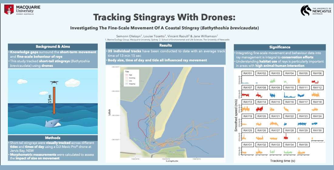
The relationship between the direction that the rays were traveling and movement was also assessed using separate linear models with mean speed and sinuosity as response variables. A Pearson’s chi-squared test was used to identify whether the direction that rays were traveling was significantly related to tide or time of day.

3. Results

3.1. Search Effort

A total of 35 tracks of short-tail stingrays were conducted between Currambene Creek and St George’s Basin during April to September 2020. As only one ray was tracked at St George’s Basin, this track was removed from most statistical analyses. The dataset and script for analysis can be found in supplementary material (S1,S2). Track times ranged from 3 min and 26 s to 26 min and 58 s (mean = 13 min and 6 s). Disc widths of tracked rays ranged from 43.33 cm to 186.13 cm (mean = 139.50 cm). A total of 53 flights were conducted with 35 finding a short-tail stingray and 18 not finding a short-tail stingray. There was no significant difference in the likelihood of finding a ray between different tides and times of day (X2 (7, n = 35) = 7.2451, p = 0.404). While flights were spread across tides and times of day, rays were not found on every possible interaction between these two factors, and as such, analyses on their possibly synergistic relationship were limited. Due to the predominantly residential status of the population of rays at Currambene Creek and an observed population size of 17 individuals [69], it is likely that the same individuals were observed on multiple occasions during separate tracks. Tracks were primarily conducted at the mouth of Currambene Creek and ray movement data were analyzed according to tide and time of day and disc width, using speed and sinuosity as key metrics (Figure 5, Figure 6 and Figure 7).

3.2. Effect of Body Size on Ray Movement

In exploring the impact of the size of the ray on its movement, disc width had a significant negative relationship with sinuosity (R2 = 0.195, F1,29 = 8.265, p = 0.008) (Figure 7), but had no significant relationship with mean speed (R2 =−0.028, F1,33 = 0.076, p = 0.785). When investigating speed using step length, however, larger rays were significantly less likely to exhibit bursts of speed greater than 1 m/s than smaller rays (X2 (1, n = 35) = 538.89, p < 0.001) (Figure 8). Disc width displayed no significant interaction with tide regarding its impact on mean speed (R2 = 0.324, F7,27 = 3.328, p = 0.011) or sinuosity (R2 = 0.187, F7,23 = 1.987, p = 0.101). Similarly, there was no significant interaction between disc width and time of day regarding its impact on mean speed (R2 = −0.019, F5,29 = 0.871, p = 0.513) or sinuosity (R2 = 0.186, F5,25 = 2.366, p = 0.069). Disc width had no significant relationship with the proportion of time a ray spent resting (R2 = 0.016, F1,33 = 1.545, p = 0.223). These results indicate that rays of different sizes were behaving similarly according to tide, time of day and the amount of time at rest.

3.3. Effect of Tide on Ray Movement

Mean speed was significantly correlated with tide (R2 = 0.25, F3,31 = 4.73, p = 0.01), with rays on average swimming faster on the high tide (mean = 0.68 m/s, n = 5) than the outgoing tide (mean = 0.38 m/s, n = 9), with a difference of 0.3 m/s (Figure 9). Looking closer at the nature of their movement, short-tail stingrays were significantly more likely to travel in bursts of speed during the high tide rather than the outgoing tide. This was shown in the significant differences in the proportion of step lengths greater than 1 m/s according to tide (X2 (3, n = 35) = 5566.20, p < 0.01), with high tide being significantly more likely to have step lengths greater than 1 m/s, and the outgoing tide being significantly less likely to have step lengths greater than 1 m/s (Figure 10). Sinuosity had no significant relationship with tide (R2 = 0.02, F3,27 = 0.78, p = 0.51). There was a significant relationship between tide and the proportion of time a ray spent resting (R2 = 0.20 F3,31 = 3.77, p = 0.02). Rays on average spent a significantly greater proportion of time resting on the outgoing tide (mean = 0.39, n = 9) than on the incoming tide (mean = 0.09, n = 11) and high tide (mean = 0.07, n = 5) (Figure 11).

3.4. Effect of Time of Day on Ray Movement

In determining the impact that time of day had on the movement of the rays, time of day had no significant relationship with either mean speed (p = 0.165, n = 35) or sinuosity (p = 0.211, n = 33), but did significantly vary the proportion of step lengths above 1 m/s (X2 (2, n = 35) = 3248, p < 0.001) (Figure 12a). Rays recorded at noon (n = 6) were much more likely to have step lengths greater than 1 m/s while those recorded in the morning (n = 23) were less likely to have step lengths greater than 1 m/s (Figure 12b). This indicates that rays were breaching this speed threshold and moving in quicker bursts during noon, while they were less likely to do so during the morning. Time of day had no significant relationship with the proportion of time a ray spent resting (R2 = −0.031, F2,32 = 0.484, p = 0.621).

3.5. Categorising Behavior

With regard to the general behavior of the rays and direction of their tracks, the ‘Stationary’ category was the only group to significantly differ from the others for mean speed (R2 = 0.617, F4,30 = 14.710, p < 0.001) (Figure 13a). Despite there being no significant relationship between direction and tide or time of day (X2 (24, n = 35) = 18.769, p = 0.764), all three tracks that were entirely stationary for the duration all occurred in the morning on an outgoing tide. Sinuosity significantly differed according to direction (R2 = 0.374, F3,27 = 6.979, p = 0.001), with rays moving downstream and upstream being less sinuous than the ‘Variable’ category and movements along the coast (Figure 13b). Stationary tracks were removed from this analysis.

4. Discussion

This study is the first to effectively utilize drones to investigate the fine-scale behavior of rays. While other approaches such as acoustic telemetry [85] and aerial surveillance from a blimp [64] have recently been used to observe the movement ecology of rays, drones present a low-cost, non-invasive opportunity to collect data for marine animals at a very high resolution. Despite criticism of the limitations presented by the battery life of drones (approximately 30 min for most quad-rotor drones such as those used in this study), tracks of rays were conducted for extended periods of time, with an average track time of 13 min and 6 s and a maximum of almost 27 min. This is an average track time approximately four times longer than those collected by Ruiz-Garcia et al. (2020) [64] using a blimp. The easy maneuverability of drones enabled tracks to occur beyond the operator’s immediate field of view, allowing for track lengths of over 800 m in this study.
No significant relationship between the sinuosity of the swim path of rays and their mean speed was observed, indicating that these short-tail stingrays did not necessarily compromise their swim speed during more sinuous swim paths. The significant negative relationship between disc width and sinuosity paired with the non-significant relationship between disc width and mean speed suggested that rays of all sizes were generally swimming at similar speeds, though larger rays were swimming in straighter swim paths. Despite there being no correlation between mean speed and disc width, larger rays were significantly less likely than smaller rays to swim in bursts of speed greater than 1 m/s. Rays had greater mean speeds and step lengths on the high tide than the outgoing tide, indicating that high tides are a period of greater activity for the rays in the estuary. The short-tail stingrays in this study were also more likely to swim in bursts of speed at noon and less likely to do so in the morning.

4.1. Effect of Body Size on Ray Movement

Animal movement varies according to the forces exerted by the morphology of the animal and the environment it inhabits [86]. Mechanisms of non-steady locomotion for animal movement, such as turning, are an area of emerging research in marine systems [87]. There is evidence that elasmobranchs operate under a U-shaped metabolism–speed curve, with an energetic minimum at intermediate cruising speeds and increasing expenditure at low and high speeds [88], and our results support this finding. For the short-tail stingrays at Currambene Creek, this intermediate cruising speed was approximately 0.5 m/s. The direction that the rays swam was not significantly related to the speed of the ray, and no relationship between ray direction and tide was observed. This suggests that regardless of the direction of the current, rays were maintaining a speed that consistently yielded maximum energetic efficiency. Whether swimming with or against the tide, rays favored the lowering of energetic costs by swimming at approximately 0.5 m/s and using the current as a means of low-energy transport, rather than swimming faster with the tide. Once again, this behavior is supported by maximum energy efficiency modeling in fish, where ignoring variations in the current and maintaining a constant speed minimizes overall energy expenditure [89].
It is possible that larger rays employed straighter swim paths to reduce the total distance traveled and avoid the energetic costs of turning more frequently. In contrast, smaller rays may have been able to swim with more tortuous trajectories and greater bursts of speed while maintaining this optimal cruising speed and minimizing excessive energy expenditure. Optimal sinuosity for foraging movements varies according to prey density and the patchiness of the environment [90], thus it is possible that smaller rays may gain advantages by swimming with greater sinuosity. Alternatively, there is evidence within elasmobranchs regarding their capacity to use learning to improve prey search and capture, as well as navigation within their home range [91]. In this way, swimming with less sinuous, straighter swim paths may be a learnt behavior in older, larger rays, maintaining a more efficient balance between energetic and foraging efficiency. The capacity for learning specifically in short-tail stingrays is demonstrated in their purportedly learnt anticipatory behavior evidenced by their increased visitation in the afternoon to the Woollamia boat ramp provisioning site within Currambene Creek, irrespective of whether the provisioning site was active [69].
Sex-related differences in stingray behavior within the estuary may offer another possible explanation for these results. Sexual dimorphism is common in batoids, with males growing to smaller sizes than females [92]. Larger resident female short-tail stingrays dominate Currambene Creek and access to the year-round food supply at the Woollamia Boat Ramp provisioning site [69], with male short-tail stingrays generally only observed within the creek approaching summer (outside the sampling dates of this study) (J. Pini-Fitzsimmons, pers. comm.). Despite this trend, it is possible that some of the rays tracked in this study were males. Male rays observed in the estuary often exhibit more erratic, possibly courting behavior as they search for and chase females (J. Pini-Fitzsimmons, pers. comm.), which may account for the higher sinuosities and greater propensity for bursts of speed. It was difficult, however, to confidently determine the presence or absence or claspers and thus the sex of the rays from the drone footage, due to varied flight altitudes and poor visibility resulting in unclear silhouettes. Future studies tracking known individuals would provide greater insight into how different sexes may be utilizing these habitats.
Less sinuous swim paths in larger rays may also be merely a morphological limitation. The turning radius in teleost fish varies according to body volume, where larger fish have a larger turning radius [93]. The functional morphology of the undulatory pectoral fin of the short-tail stingray is, however, substantially different from the body morphology of teleosts [94]. Furthermore, different species of rays with similar morphologies to short-tail stingrays can rotate their bodies with an essentially zero turning radius [95], making this explanation less plausible. In our study, rays of all sizes swam with greater sinuosity outside the mouth of the estuary where substrate was more complex and varied, and with less sinuosity when traveling up and down the estuary, indicating that the size of the ray was not the only determinant of sinuosity.

4.2. Effect of Tide on Ray Movement

The tidal cycle may instigate different behaviors for rays, with greater mean speeds at high tide compared to the outgoing tide. Atlantic cownose rays (Rhinoptera bonasus) feed during the high tide before retreating to intertidal waters during the outgoing tide [39]. This may explain the increased activity of the short-tail stingrays at Currambene Creek during the high tide, with individuals swimming with greater speed as they search for food or travel to feeding grounds. Exposed sandbars also become submerged during the high tide, giving rays the opportunity to swim freely, avoiding the high boating traffic, dredged boating channel and accessing more feeding sites, though no obvious feeding behaviors were identified from the drone footage. The presence of the provisioning site within the estuary to which many of the residential individuals make regular visits [69] may relieve the pressure for these rays to invest time and energy foraging for their own food. Instead, increases in activity during the high tide may reflect the increased flow of water and greater water visibility, particularly compared to low and outgoing tides. The importance of high tide for ray ecology as a period of higher activity when rays are likely to be traveling up and down the estuary should be considered in management strategies when balancing increases in boating and fishing activity similarly concentrated around high tide.
The reduced activity of rays around the outgoing tide could be linked to energetic limitations. There is evidence of thermoregulatory behavior in rays [96], driven by the effects of temperature on ray metabolism and energy expenditure [33]. Many rays have seasonal movements to deeper waters [35,97,98], particularly in winter, perhaps to slow down their metabolism. Short-tail stingrays are found at depths up to 480 m [68], indicating tolerances and perhaps preferences for cooler waters, which may impact their fine-scale behavior. Rays may swim slower to avoid unnecessary energy expenditure during the outgoing tide when water temperatures may be higher as warmer water flows downstream from the shallows of the upper estuary. Then, as cooler water from the bay fills the estuary at high tide, rays may maintain optimal metabolic rates at higher swim speeds. In this scenario, rays are attempting to maintain their rate of energy expenditure close to their basal metabolic rate, where warmer water pushes them higher within their metabolic scope, causing a compensation for this by regulating their swim speed. This is further supported by the negative relationship observed with time spent resting on both the high and incoming tide. These trends, however, should be paired with the further monitoring of water temperature data from the estuary at a similarly high resolution to the drone data to more fully understand this relationship.

4.3. Effect of Time of Day on Ray Movement

Step length, which provides insight into the nature of movement during the track [82], was significantly related to time of day. Short-tail stingrays in this study were more likely to swim in bursts of speed at noon and less likely to do so in the morning. It is possible that as boating activity increases towards noon, rays may employ these quick bursts of speed to avoid boats more often at these times. Short-tail stingrays have sensitive mechanoreceptors [99] and were often observed to rapidly alter their swim paths or perform fast starts off the substrate from a resting position to evade oncoming boats in a behavior akin to predator avoidance [95,100]. Elasmobranchs display more intense escape responses as the speed and size of predators increases [101].
Despite evidence that various ray species may be more active at night [45,102], there is only limited evidence to suggest this is true for the short-tail stingray [34], with a clear concentration of bursts of speed at noon observed in this study. Although the retinas of short-tail stingrays have a lower rod to cone ratio than other rays [103], the presence of a reflective layer in front of the photoreceptors, known as the tapetum lucidum, indicates that short-tail stingrays are adapted to poorly illuminated ecosystems [104], making them especially sensitive to bright light. This may explain these bursts of speed during noon when light intensity is often highest, eliciting more intense responses to environmental stimuli at this time of day. Day-time inactivity and night-time activity may be a predator avoidance strategy in rays [105]. In this way, the short-tail stingrays may be more active within the estuary where predators are unlikely to enter during the day, and more active in the bay at night as they forage for nocturnally active prey. Predator avoidance has been downplayed as a key driver in the movement of short-tail stingrays due to the lack of real predation pressure, with few large predators capable of preying on rays of this size [34]. However, white sharks (Carcharodon carcharias) are a known predator of the short-tail stingray and impact the behavior of short-tail stingrays around shark cage diving sites [106]. White sharks are often sighted within Jervis Bay, suggesting this pressure may be real for the population at Currambene Creek for rays that have experienced white shark predation pressure in the wider bay area.

4.4. Site and Species Considerations

While investigating the fine-scale movement of an animal within its ecosystem at a high resolution, it is important to consider how species-specific and site-specific variables influence movement at a resolution that is ecologically relevant to the animal. Little is known about the ecological habits of the short-tail stingray due to identification confusion with other large batoids with a similar physiology and distribution, such as the brown stingray (Bathytoshia lata), as well as a general lack of biological research on the species [68]. The short-tail stingray grows to a maximum disc width exceeding 210 cm, but is pupped with a disc width of just 32–36 cm [107], making it probable that different movement behaviors emerge as their size increases. Movement of rays up and down Currambene Creek are likely to be affected by the provisioning site located further up the estuary, increasing the probability of traveling behaviors to this site, particularly in the afternoon when fishers are cleaning their catch [69]. Rays were consistently found in the dredged channel within the estuary and showed little reaction to moored boats, but would often flurry away from nearby moving boats, particularly at shallower depths (Oleksyn, unpublished data). Short-tail stingrays alter their swimming behavior in shallow environments in close proximity to swimmers [64]. While it is possible that similar animal–human interactions would occur at Currambene Creek, none were observed during this study.

5. Conclusions

This study has demonstrated the effectiveness of drones in obtaining high-resolution movement data for stingrays. The data collected in this study indicate that the fine-scale movement behavior of rays can be driven by a range of factors including tide, time of day and the size of the ray. The analysis of the possibly synergistic relationship between these factors and others such as direction was limited by sample size, but they are likely to interact in a significant manner, and further research is required to understand these ecological dynamics. Pairing aerial observations of fine-scale movement with longer-term tagging studies will help elucidate the drivers of movement in a more holistic manner. The resident population of short-tail stingrays at Currambene Creek act as a model for other ray populations occupying coastal estuaries in proximity to human settlements. Human activities have the potential to interact significantly with natural variables, such as tide and time of day, in driving the fine-scale movement of marine animals such as rays. Considering this potential is important when developing management strategies with objectives to support the natural movements and behavior of rays and other animals.

Supplementary Materials

The following are available online at https://www.mdpi.com/2072-4292/13/1/40/s1, (S1) RayTracking.r, script for the analyses performed here and (S2) Jervis Traj Data.csv, dataset.

Author Contributions

Conceptualization, S.O.; L.T.; V.R.; J.E.W.; methodology, S.O.; L.T.; V.R.; J.E.W.; software, S.O.; L.T.; V.R.; validation, S.O.; L.T.; formal analysis, S.O.; L.T.; V.R.; investigation, S.O.; resources, S.O.; V.R.; J.E.W.; data curation, S.O.; writing—original draft preparation, S.O.; writing—review and editing, L.T.; V.R.; J.E.W.; visualization, S.O.; supervision, L.T.; V.R.; J.E.W.; project administration, S.O.; J.E.W.; funding acquisition, S.O.; J.E.W. All authors have read and agreed to the published version of the manuscript.

Funding

This research was funded by the Department of Biological Sciences at Macquarie University and the Rice Memorial Field Research Award 2020. Semonn Oleksyn was supported by the Macquarie University RTP Scholarship.

Institutional Review Board Statement

The study was conducted according to the guidelines of the Australian code for the care and use of animals for scientific purposes, and approved by the Animal Ethics Committee of Macquarie University (ARA 2019/012, approved 14/3/19).

Informed Consent Statement

Not applicable.

Data Availability Statement

The data presented in this study are available in Supplementary Materials.

Acknowledgments

We wish to thank Joni Pini-Fitzsimmons for her co-operation during this project. Her knowledge on the short-tail stingray and the population at Jervis Bay was greatly appreciated. We thank Troy Gaston for the use of his drone.

Conflicts of Interest

The authors declare no conflict of interest.

References

  1. Fahrig, L. Non-optimal animal movement in human-altered landscapes. Funct. Ecol. 2007, 21, 1003–1015. [Google Scholar] [CrossRef]
  2. Doherty, T.S.; Driscoll, D.A. Coupling movement and landscape ecology for animal conservation in production landscapes. Proc. R. Soc. B Biol. Sci. 2018, 285, 20172272. [Google Scholar] [CrossRef]
  3. Halpern, B.S.; Walbridge, S.; Selkoe, K.A.; Kappel, C.V.; Micheli, F.; Agrosa, C.; Watson, R. A Global Map of Human Impact on Marine Ecosystems. Science 2008, 319, 948–952. [Google Scholar] [CrossRef] [Green Version]
  4. Halpern, B.S.; Frazier, M.; Potapenko, J.; Casey, K.S.; Koenig, K.; Longo, C.; Walbridge, S. Spatial and temporal changes in cumulative human impacts on the world’s ocean. Nat. Commun. 2015, 6, 7615. [Google Scholar] [CrossRef] [Green Version]
  5. Jackson, J.B.C.; Kirby, M.X.; Berger, W.H.; Bjorndal, K.A.; Botsford, L.W.; Bourque, B.J.; Warner, R.R. Historical Overfishing and the Recent Collapse of Coastal Ecosystems. Science 2001, 293, 629–637. [Google Scholar] [CrossRef] [Green Version]
  6. He, Q.; Silliman, B.R. Climate Change, Human Impacts, and Coastal Ecosystems in the Anthropocene. Curr. Biol. 2019, 29, R1021–R1035. [Google Scholar] [CrossRef]
  7. Beck, M.W.; Heck, K.L.; Able, K.W.; Childers, D.L.; Eggleston, D.B.; Gillanders, B.M.; Minello, T.J. The Role of Nearshore Ecosystems as Fish and Shellfish Nurseries. 2003. Available online: https://www.epa.gov/watershedacademy/role-nearshore-ecosystems-fish-and-shellfish-nurseries (accessed on 3 December 2020).
  8. Sheaves, M.; Baker, R.; Nagelkerken, I.; Connolly, R.M. True value of estuarine and coastal nurseries for fish: Incorporating complexity and dynamics. Estuaries Coasts 2015, 38, 401–414. [Google Scholar] [CrossRef] [Green Version]
  9. Fauchald, P.; Tveraa, T. Hierarchical patch dynamics and animal movement pattern. Oecologia 2006, 149, 383–395. [Google Scholar] [CrossRef]
  10. Schofield, G.; Katselidis, K.A.; Lilley, M.K.S.; Reina, R.D.; Hays, G.C. Detecting elusive aspects of wildlife ecology using drones: New insights on the mating dynamics and operational sex ratios of sea turtles. Funct. Ecol. 2017, 31, 2310–2319. [Google Scholar] [CrossRef]
  11. Feinsinger, P.; Colwell, R.K.; Terborgh, J.; Chaplin, S.B. Elevation and the Morphology, Flight Energetics, and Foraging Ecology of Tropical Hummingbirds. Am. Nat. 1979, 113, 481–497. [Google Scholar] [CrossRef]
  12. Braña, F. Morphological correlates of burst speed and field movement patterns: The behavioural adjustment of locomotion in wall lizards (Podarcis muralis). Biol. J. Linn. Soc. 2003, 80, 135–146. [Google Scholar] [CrossRef] [Green Version]
  13. Braccini, M.; Aires-Da-Silva, A.; Taylor, I. Incorporating movement in the modelling of shark and ray population dynamics: Approaches and management implications. Rev. Fish Biol. Fish. 2016, 26, 13–24. [Google Scholar] [CrossRef]
  14. Porreca, A.P.; Hintz, W.D.; Whitledge, G.W.; Rude, N.P.; Heist, E.J.; Garvey, J.E. Establishing ecologically relevant management boundaries: Linking movement ecology with the conservation of Scaphirhynchus sturgeon. Can. J. Fish. Aquat. Sci. 2016, 73, 877–884. [Google Scholar] [CrossRef]
  15. Ogburn, M.B.; Harrison, A.-L.; Whoriskey, F.G.; Cooke, S.J.; Mills Flemming, J.E.; Torres, L.G. Addressing Challenges in the Application of Animal Movement Ecology to Aquatic Conservation and Management. Front. Mar. Sci. 2017, 4, 70. Available online: https://www.frontiersin.org/article/10.3389/fmars.2017.00070 (accessed on 3 December 2020). [CrossRef] [Green Version]
  16. Allen, A.M.; Singh, N.J. Linking Movement Ecology with Wildlife Management and Conservation. Front. Ecol. Evol. 2016, 3, 155. Available online: https://www.frontiersin.org/article/10.3389/fevo.2015.00155 (accessed on 3 December 2020). [CrossRef] [Green Version]
  17. Katzner, T.; Arlettaz, R. Evaluating Contributions of Recent Tracking-Based Animal Movement Ecology to Conservation Management. Front. Ecol. Evol. 2019, 7, 519. [Google Scholar] [CrossRef] [Green Version]
  18. Stein, R.W.; Mull, C.G.; Kuhn, T.S.; Aschliman, N.C.; Davidson, L.N.K.; Joy, J.B.; Mooers, A.O. Global priorities for conserving the evolutionary history of sharks, rays and chimaeras. Nat. Ecol. Evol. 2018, 2, 288–298. [Google Scholar] [CrossRef] [PubMed]
  19. O’Shea, O.R.; Thums, M.; van Keulen, M.; Meekan, M. Bioturbation by stingrays at Ningaloo Reef, Western Australia. Mar. Freshw. Res. 2012, 63, 189–197. [Google Scholar] [CrossRef] [Green Version]
  20. Bornatowski, H.; Navia, A.F.; Braga, R.R.; Abilhoa, V.; Corrêa, M.F.M. Ecological importance of sharks and rays in a structural foodweb analysis in southern Brazil. ICES J. Mar. Sci. 2014, 71, 1586–1592. [Google Scholar] [CrossRef] [Green Version]
  21. Flowers, K.I.; Heithaus, M.R.; Papastamatiou, Y.P. Buried in the sand: Uncovering the ecological roles and importance of rays. Fish Fish. 2020. [Google Scholar] [CrossRef]
  22. Young, H.J.; Raoult, V.; Platell, M.E.; Williamson, J.E.; Gaston, T.F. Within-genus differences in catchability of elasmobranchs during trawling. Fish. Res. 2019, 211, 141–147. [Google Scholar] [CrossRef]
  23. Dulvy, N.K.; Baum, J.K.; Clarke, S.; Compagno, L.J.V.; Cortés, E.; Domingo, A.; Gibson, C. You can swim but you can’t hide: The global status and conservation of oceanic pelagic sharks and rays. Aquat. Conserv. Mar. Freshw. Ecosyst. 2008, 18, 459–482. [Google Scholar] [CrossRef]
  24. Dulvy, N.K.; Fowler, S.L.; Musick, J.A.; Cavanagh, R.D.; Kyne, P.M.; Harrison, L.R.; White, W.T. Extinction risk and conservation of the world’s sharks and rays. Elife 2014, 3. [Google Scholar] [CrossRef] [PubMed] [Green Version]
  25. Field, I.C.; Meekan, M.G.; Buckworth, R.C.; Bradshaw, C.J.A. Susceptibility of sharks, rays and chimaeras to global extinction. Adv. Mar. Biol. 2009, 56, 275–363. [Google Scholar] [PubMed]
  26. Rogers, C.; Roden, C.; Lohoefener, R.; Mullin, K.; Hoggard, W. Behavior, distribution, and relative abundance of cownose ray schools Rhinoptera bonasus in the northern Gulf of Mexico. Gulf Mex. Sci. 1990, 11, 8. [Google Scholar] [CrossRef]
  27. James, P. Observations on shoals of the Javanese Cownose Ray Rhinoptera javanica Muller & Henle from the Gulf of Mannar, with additional notes on the species. J. Mar. Biol. Assoc. India 1962, 4, 217–223. [Google Scholar]
  28. Schwartz, F.J. Mass Migratory Congregations and Movements of Several Species of Cownose Rays, Genus Rhinoptera: A World-Wide Review. J. Elisha Mitchell Sci. Soc. 1990, 106, 10–13. Available online: www.jstor.org/stable/24333475 (accessed on 3 December 2020).
  29. Merriner, J.V.; Smith, J.W. A report to the oyster industry of Virginia on the biology and management of the cownose ray (Rhinoptera bonasus, Mitchill) in lower Chesapeake Bay. Spec. Rep. Appl. Mar. Sci. Ocean Eng. 1979, 216, 957. [Google Scholar]
  30. Smith, J.W.; Merriner, J. Observations on The Reproductive-Biology of The Cownose Ray, Rhinoptera-Bonasus, In Chesapeake Bay. Fish. Bull. 1986, 84, 871. [Google Scholar]
  31. Smith, J.W.; Merriner, J.V. Age and Growth, Movements and Distribution of the Cownose Ray, Rhinoptera bonasus, in Chesapeake Bay. Estuaries 1987, 10, 153. [Google Scholar] [CrossRef]
  32. Gray, A.E.; Mulligan, T.J.; Hannah, R.W. Food habits, occurrence, and population structure of the bat ray, Myliobatis californica, in Humboldt Bay, California. Environ. Biol. Fishes 1997, 49, 227–238. [Google Scholar] [CrossRef]
  33. Hopkins, T.E.; Cech, J.J. Effect of temperature on oxygen consumption of the bat ray, Myliobatis californica (Chondrichthyes, Myliobatididae). Copeia 1994, 529–532. [Google Scholar] [CrossRef]
  34. Le Port, A.; Sippel, T.; Montgomery, J.C. Observations of mesoscale movements in the short-tailed stingray, Dasyatis brevicaudata from New Zealand using a novel PSAT tag attachment method. J. Exp. Mar. Biol. Ecol. 2008, 359, 110–117. [Google Scholar] [CrossRef]
  35. Le Port, A.; Lavery, S.; Montgomery, J.C. Conservation of coastal stingrays: Seasonal abundance and population structure of the short-tailed stingray Dasyatis brevicaudata at a Marine Protected Area. ICES J. Mar. Sci. 2012, 69, 1427–1435. [Google Scholar] [CrossRef] [Green Version]
  36. Collins, A.B.; Heupel, M.R.; Simpfendorfer, C.A. Spatial Distribution and Long-term Movement Patterns of Cownose Rays Rhinoptera bonasus Within an Estuarine River. Estuaries Coasts 2008, 31, 1174–1183. [Google Scholar] [CrossRef]
  37. Drymon, J.M. Distributions of Coastal Sharks in the Northern Gulf of Mexico: Consequences for Trophic Transfer and Foodweb Dynamics; University of South Alabama: Mobile, Alabama, 2010. [Google Scholar]
  38. Ajemian, M.J.; Powers, S.P. Seasonality and Ontogenetic Habitat Partitioning of Cownose Rays in the Northern Gulf of Mexico. Estuaries Coasts 2016, 39, 1234–1248. [Google Scholar] [CrossRef]
  39. Smith, J.W.; Merriner, J.V. Food Habits and Feeding Behavior of the Cownose Ray, Rhinoptera bonasus, in Lower Chesapeake Bay. Estuaries 1985, 8, 305. [Google Scholar] [CrossRef]
  40. Coles, R.J. Observations on the Habits and Distribution of Certain Fishes Taken on the Coast of North Carolina; Order of the Trustees; American Museum of Natural History: New York, NY, USA, 1910. [Google Scholar]
  41. Davy, L.E.; Simpfendorfer, C.A.; Heupel, M.R. Movement patterns and habitat use of juvenile mangrove whiprays (Himantura granulata). Mar. Freshw. Res. 2015, 66, 481. [Google Scholar] [CrossRef]
  42. Kanno, S.; Schlaff, A.; Heupel, M.; Simpfendorfer, C. Stationary video monitoring reveals habitat use of stingrays in mangroves. Mar. Ecol. Prog. Ser. 2019, 621, 155–168. [Google Scholar] [CrossRef]
  43. Martins, A.P.B.; Heupel, M.R.; Bierwagen, S.L.; Chin, A.; Simpfendorfer, C. Diurnal activity patterns and habitat use of juvenile Pastinachus ater in a coral reef flat environment. PLoS ONE 2020, 15, e0228280. [Google Scholar] [CrossRef] [Green Version]
  44. Hoisington, G.; Lowe, C.G. Abundance and distribution of the round stingray, Urobatis halleri, near a heated effluent outfall. Mar. Environ. Res. 2005, 60, 437–453. [Google Scholar] [CrossRef] [PubMed]
  45. Vaudo, J.J.; Lowe, C.G. Movement patterns of the round stingray Urobatis halleri (Cooper) near a thermal outfall. J. Fish Biol. 2006, 68, 1756–1766. [Google Scholar] [CrossRef] [Green Version]
  46. Matern, S.A.; Cech, J.J.; Hopkins, T.E. Diel movements of bat rays, Myliobatis californica, in Tomales Bay, California: Evidence for behavioral thermoregulation? Environ. Biol. Fishes 2000, 58, 173–182. [Google Scholar] [CrossRef]
  47. Tagliafico, A.; Butcher, P.A.; Colefax, A.P.; Clark, G.F.; Kelaher, B.P. Variation in cownose ray Rhinoptera neglecta abundance and group size on the central east coast of Australia. J. Fish Biol. 2019. [Google Scholar] [CrossRef] [PubMed]
  48. Crossin, G.T.; Hinch, S.G.; Farrell, A.P.; Higgs, D.A.; Lotto, A.G.; Oakes, J.D.; Healey, M.C. Energetics and morphology of sockeye salmon: Effects of upriver migratory distance and elevation. J. Fish Biol. 2004, 65, 788–810. [Google Scholar] [CrossRef]
  49. Pettersson, L.B.; Hedenström, A. Energetics, cost reduction and functional consequences of fish morphology. Proc. R. Soc. Lond. Ser. B Biol. Sci. 2000, 267, 759–764. [Google Scholar] [CrossRef] [Green Version]
  50. Schlaff, A.M.; Heupel, M.R.; Simpfendorfer, C.A. Influence of environmental factors on shark and ray movement, behaviour and habitat use: A review. Rev. Fish Biol. Fish. 2014, 24, 1089–1103. [Google Scholar] [CrossRef]
  51. Strong, W.R.; Snelson, F.F.; Gruber, S.H. Hammerhead Shark Predation on Stingrays: An Observation of Prey Handling by Sphyrna mokarran. Copeia 1990, 836–840. [Google Scholar] [CrossRef]
  52. Myers, R.A.; Baum, J.K.; Shepherd, T.D.; Powers, S.P.; Peterson, C.H. Cascading Effects of the Loss of Apex Predatory Sharks from a Coastal Ocean. Science 2007, 315, 1846–1850. [Google Scholar] [CrossRef]
  53. Heithaus, M.R.; Frid, A.; Wirsing, A.J.; Worm, B. Predicting ecological consequences of marine top predator declines. Trends Ecol. Evol. 2008, 23, 202–210. [Google Scholar] [CrossRef]
  54. Bond, M.E.; Valentin-Albanese, J.; Babcock, E.A.; Heithaus, M.R.; Grubbs, R.D.; Cerrato, R.; Chapman, D.D. Top predators induce habitat shifts in prey within marine protected areas. Oecologia 2019, 190, 375–385. [Google Scholar] [CrossRef] [PubMed]
  55. Semeniuk, C.A.D.; Rothley, K.D. Costs of group-living for a normally solitary forager: Effects of provisioning tourism on southern stingrays Dasyatis americana. Mar. Ecol. Prog. Ser. 2008, 357, 271–282. [Google Scholar] [CrossRef]
  56. Lobel, P.S. Underwater acoustic ecology: Boat noises and fish behavior. In Proceedings of the AAUS Diving for Science 2009 Symposium, Atlanta, GA, USA, 13–14 March 2009; pp. 31–42. [Google Scholar]
  57. Caldwell, I.R.; Gergel, S.E. Thresholds in seascape connectivity: Influence of mobility, habitat distribution, and current strength on fish movement. Landsc. Ecol. 2013, 28, 1937–1948. [Google Scholar] [CrossRef]
  58. Berthe, C.; Lecchini, D. Influence of boat noises on escape behaviour of white-spotted eagle ray Aetobatus ocellatus at Moorea Island (French Polynesia). Compt. Rendus Biol. 2016, 339, 99–103. [Google Scholar] [CrossRef]
  59. Simpson, S.D.; Radford, A.N.; Nedelec, S.L.; Ferrari, M.C.O.; Chivers, D.P.; McCormick, M.I.; Meekan, M.G. Anthropogenic noise increases fish mortality by predation. Nat. Commun. 2016, 7, 10544. [Google Scholar] [CrossRef] [PubMed] [Green Version]
  60. Butcher, P.C.; Kajiura, S.M.; Lopez, N.A.; Mourier, J.; Purcell, C.R.; Skomal, G.B.; Tucker, J.P.; Walsh, A.J.; Williamson, J.E.; Raoult, V.; et al. The Drone Revolution of Shark Science: A Review. Drones. (under review).
  61. Lower, N.; Moore, A.; Scott, A.P.; Ellis, T.; James, J.D.; Russell, I.C. A non-invasive method to assess the impact of electronic tag insertion on stress levels in fishes. J. Fish Biol. 2005, 67, 1202–1212. [Google Scholar] [CrossRef]
  62. Klefoth, T.; Kobler, A.; Arlinghaus, R. The impact of catch-and-release angling on short-term behaviour and habitat choice of northern pike (Esox lucius L.). Hydrobiologia 2008, 601, 99–110. [Google Scholar] [CrossRef]
  63. Jepsen, N.; Thorstad, E.B.; Havn, T.; Lucas, M.C. The use of external electronic tags on fish: An evaluation of tag retention and tagging effects. Anim. Biotelemetry 2015, 3, 49. [Google Scholar] [CrossRef] [Green Version]
  64. Ruiz-García, D.; Adams, K.; Brown, H.; Davis, A.R. Determining Stingray Movement Patterns in a Wave-Swept Coastal Zone Using a Blimp for Continuous Aerial Video Surveillance. Fishes 2020, 5, 31. [Google Scholar] [CrossRef]
  65. Oleksyn, S.; Tosetto, L.; Raoult, V.; Joyce, K.; Williamson, J.E. Going Batty: The Challenges and Opportunities for Drone Researchers In Monitoring Behaviour And Habitat Use Of Rays. Drones. (under review).
  66. Christiansen, F.; Rojano-Doñate, L.; Madsen, P.T.; Bejder, L. Noise Levels of Multi-Rotor Unmanned Aerial Vehicles with Implications for Potential Underwater Impacts on Marine Mammals. Front. Mar. Sci. 2016, 3, 277. Available online: https://www.frontiersin.org/article/10.3389/fmars.2016.00277 (accessed on 3 December 2020). [CrossRef] [Green Version]
  67. Mulero-Pázmány, M.; Jenni-Eiermann, S.; Strebel, N.; Sattler, T.; Negro, J.J.; Tablado, Z. Unmanned aircraft systems as a new source of disturbance for wildlife: A systematic review. PLoS ONE 2017, 12, e0178448. [Google Scholar] [CrossRef] [PubMed] [Green Version]
  68. Duffy, C.A.J.; Paul, L.J.; Chin, A. Bathytoshia brevicaudata. The IUCN Red List of Threatened Species 2016. 2016. Available online: https://dx.doi.org/10.2305/IUCN.UK.2016-1.RLTS.T41796A68618154.en (accessed on 3 December 2020).
  69. Pini-Fitzsimmons, J.; Knott, N.; Brown, C. Effects of food provisioning on site use in the short-tail stingray Bathytoshia brevicaudata. Mar. Ecol. Prog. Ser. 2018, 600, 99–110. [Google Scholar] [CrossRef]
  70. Last, P.R.; Manjaji-Matsumoto, B.M.; Naylor, G.J.P.; White, W.T. 25. Stingrays. Family Dasyatidae. Rays World. Csiro Publ. Comstock Publ. Assoc. Ithaca Lond. 2016, 1, 522–618. [Google Scholar]
  71. Raoult, V.; Tosetto, L.; Williamson, E.J. Drone-Based High-Resolution Tracking of Aquatic Vertebrates. Drones 2018, 2, 37. [Google Scholar] [CrossRef] [Green Version]
  72. Hugenholtz, C.; Brown, O.; Walker, J.; Barchyn, T.; Nesbit, P.; Kucharczyk, M.; Myshak, S. Spatial accuracy of UAV-derived orthoimagery and topography: Comparing photogrammetric models processed with direct geo-referencing and ground control points. Geomatica 2016, 70, 21–30. [Google Scholar] [CrossRef]
  73. Colefax, A.P.; Kelaher, B.P.; Pagendam, D.E.; Butcher, P.A. Assessing White Shark (Carcharodon carcharias) Behavior Along Coastal Beaches for Conservation-Focused Shark Mitigation. Front. Mar. Sci. 2020, 7, 268. [Google Scholar] [CrossRef]
  74. Microsoft Corporation. Microsoft Excel. 2020. Available online: https://office.microsoft.com/excel (accessed on 3 December 2020).
  75. R Core Team. R: A Language and Environment for Statistical Computing; R Foundation for Statistical Computing: Vienna, Austria, 2020; Available online: https://www.R-project.org/ (accessed on 3 December 2020).
  76. RStudio Team. RStudio: Integrated Development for R; RStudio, Inc.: Boston, MA, USA, 2019; Available online: http://www.rstudio.com/ (accessed on 3 December 2020).
  77. NSW Department of Planning, Industry, and Environment. Currambene Creek. 2018. Available online: https://www.environment.nsw.gov.au/topics/water/estuaries/estuaries-of-nsw/currambene-creek (accessed on 3 December 2020).
  78. Scheider, C.A.; Rasband, W.S.; Eliceiri, K.W. NIH ImageJ: 25 years of image analysis. Nat. Methods 2012, 9, 671–675. [Google Scholar] [CrossRef]
  79. Kahle, D.; Wickham, H. ggmap: Spatial Visualization with ggplot2. R J. 2013, 5, 144–161. [Google Scholar] [CrossRef] [Green Version]
  80. Bivand, R.; Keitt, T.; Rowlingson, B.; Pebesma, E.; Sumner, M.; Hijmans, R.; Bivand, M.R. Package ‘rgdal’. Bind. Geospat. Data Abstr. Libr. 2015. Available online: https://cran.r-project.org/web/packages/rgdal/index.html (accessed on 3 December 2020).
  81. McLean, D.J.; Skowron Volponi, M.A. trajr: An R package for characterisation of animal trajectories. Ethology 2018, 124, 440–448. [Google Scholar] [CrossRef] [Green Version]
  82. Edelhoff, H.; Signer, J.; Balkenhol, N. Path segmentation for beginners: An overview of current methods for detecting changes in animal movement patterns. Mov. Ecol. 2016, 4, 21. [Google Scholar] [CrossRef] [PubMed] [Green Version]
  83. Bainbridge, R. The Speed of Swimming of Fish as Related to Size and to the Frequency and Amplitude of the Tail Beat. J. Exp. Biol. 1958, 35, 109. Available online: http://jeb.biologists.org/content/35/1/109.abstract (accessed on 3 December 2020).
  84. Ware, D.M. Bioenergetics of Pelagic Fish: Theoretical Change in Swimming Speed and Ration with Body Size. J. Fish. Res. Board Can. 1978, 35, 220–228. [Google Scholar] [CrossRef]
  85. Martins, A.P.B.; Heupel, M.R.; Oakley-Cogan, A.; Chin, A.; Simpfendorfer, C.A. Towed-float GPS telemetry: A tool to assess movement patterns and habitat use of juvenile stingrays. Mar. Freshw. Res. 2019, 71, 89–98. [Google Scholar] [CrossRef]
  86. Dickinson, M.H. How Animals Move: An Integrative View. Science 2000, 288, 100–106. [Google Scholar] [CrossRef] [Green Version]
  87. Daley, M.A.; Bertram, J. Non-steady locomotion. In Understanding Mammalian Locomotion: Concepts and Applications; John Wiley & Sons: Hoboken, NJ, USA, 2016; pp. 277–306. [Google Scholar]
  88. Di Santo, V.; Kenaley, C.P.; Lauder, G.V. High postural costs and anaerobic metabolism during swimming support the hypothesis of a U-shaped metabolism–speed curve in fishes. Proc. Natl. Acad. Sci. USA 2017, 114, 13048–13053. [Google Scholar] [CrossRef] [Green Version]
  89. Trump, C.L.; Leggett, W.C. Optimum swimming speeds in fish: The problem of currents. Can. J. Fish. Aquat. Sci. 1980, 37, 1086–1092. [Google Scholar] [CrossRef]
  90. Bovet, P.; Benhamou, S. Optimal sinuosity in central place foraging movements. Anim. Behav. 1991, 42, 57–62. [Google Scholar] [CrossRef]
  91. Guttridge, T.L.; Myrberg, A.A.; Porcher, I.F.; Sims, D.W.; Krause, J. The role of learning in shark behaviour. Fish Fish. 2009, 10, 450–469. [Google Scholar] [CrossRef]
  92. Henningsen, A.D.; Leaf, R.T. Observations on the Captive Biology of the Southern Stingray. Trans. Am. Fish. Soc. 2010, 139, 783–791. [Google Scholar] [CrossRef]
  93. Webb, P.W. Speed, Acceleration and Manoeuvrability of Two Teleost Fishes. J. Exp. Biol. 1983, 102, 115. Available online: http://jeb.biologists.org/content/102/1/115.abstract (accessed on 3 December 2020).
  94. Rosenberger, L.J.; Westneat, M.W. Functional morphology of undulatory pectoral fin locomotion in the stingray taeniura lymma (Chondrichthyes: Dasyatidae). J. Exp. Biol. 1999, 202, 3523. Available online: http://jeb.biologists.org/content/202/24/3523.abstract (accessed on 3 December 2020). [PubMed]
  95. Seamone, S.G.; McCaffrey, T.M.; Syme, D.A. Disc starts: The pectoral disc of stingrays promotes omnidirectional fast starts across the substrate. Can. J. Zool. 2019, 97, 597–605. [Google Scholar] [CrossRef]
  96. Casella, E.; Collin, A.; Harris, D.; Ferse, S.; Bejarano, S.; Parravicini, V.; Rovere, A. Mapping coral reefs using consumer-grade drones and structure from motion photogrammetry techniques. Coral Reefs 2017, 36, 269–275. [Google Scholar] [CrossRef]
  97. Snelson, F.F. Notes on the occurrence, distribution, and biology of elasmobranch fishes in the Indian River lagoon system, Florida. Estuaries 1981, 4, 110–120. [Google Scholar] [CrossRef]
  98. Walker, P.; Howlett, G.; Millner, R. Distribution, movement and stock structure of three ray species in the North Sea and eastern English Channel. ICES J. Mar. Sci. 1997, 54, 797–808. [Google Scholar] [CrossRef]
  99. Montgomery, J.; Skipworth, E. Detection of Weak Water Jets by the Short-Tailed Stingray Dasyatis brevicaudata (Pisces: Dasyatidae). Copeia 1997, 4, 881–883. [Google Scholar] [CrossRef]
  100. Semeniuk, C.A.D.; Dill, L.M. Anti-Predator Benefits of Mixed-Species Groups of Cowtail Stingrays (Pastinachus sephen) and Whiprays (Himantura uarnak) at Rest. Ethology 2006, 112, 33–43. [Google Scholar] [CrossRef]
  101. Seamone, S.; Blaine, T.; Higham, T.E. Sharks modulate their escape behavior in response to predator size, speed and approach orientation. Zoology 2014, 117, 377–382. [Google Scholar] [CrossRef]
  102. Brinton, C.P.; Curran, M.C. Tidal and diel movement patterns of the Atlantic stingray (Dasyatis sabina) along a stream-order gradient. Mar. Freshw. Res. 2017, 68, 1716. [Google Scholar] [CrossRef]
  103. Braekevelt, C.R. Retinal photoreceptor fine structure in the short-tailed stingray Dasyatis brevicaudata. Histol. Histopathol. 1994, 9, 507–514. [Google Scholar] [PubMed]
  104. Braekevelt, C.R. Fine structure of the tapetum lucidum in the short-tailed stingray Dasyatis brevicaudata. Histol. Histopathol. 1994, 9, 495–500. [Google Scholar] [PubMed]
  105. Cartamil, D.P.; Vaudo, J.J.; Lowe, C.G.; Wetherbee, B.M.; Holland, K.N. Diel movement patterns of the Hawaiian stingray, Dasyatis lata: Implications for ecological interactions between sympatric elasmobranch species. Mar. Biol. 2003, 142, 841–847. [Google Scholar] [CrossRef]
  106. Rizzari, J.R.; Semmens, J.M.; Fox, A.; Huveneers, C. Observations of marine wildlife tourism effects on a non-focal species. J. Fish Biol. 2017, 91, 981–988. [Google Scholar] [CrossRef]
  107. Last, P.R.; Stevens, J.D. Sharks and Rays of Australia; CSIRO Australia: East Melbourne, Australia, 1994.
Figure 1. (a) Model mature (large) and (b) juvenile (small) short-tail stingrays. All measurements are shown in centimeters. (c) Calibration curve plotting the pixels per centimeter of the ray models against the drone altitude using measurements from both the small and large models at ten different altitudes. The shaded area represents the 95% confidence intervals. (df) Drone images of model stingrays. Images were taken in sheltered waters with <10 kph winds. Image (d) was taken at 5 m altitude, (e) at 20 m altitude and (f) at 50 m altitude.
Remotesensing 13 00040 g001
Figure 2. Conceptual diagram of step length from Edelhoff et al. 2016 [82].
Remotesensing 13 00040 g002
Figure 3. Speed profiles of RAY01 (a) and RAY22 (b) tracks. The red line indicates the resting threshold set at 0.2 m/s. The blue shading indicates a period of more than 5 s below the threshold. RAY01 displayed resting behavior in the drone footage, while RAY22 was swimming for the entire duration.
Remotesensing 13 00040 g003
Figure 4. Step lengths during all ray tracks. The red line indicates a drop-off in frequency at a step length of 0.1 m/100 ms.
Remotesensing 13 00040 g004
Figure 5. Tracks of short-tail stingrays, plotted according to tide (a) and time of day (b), overlayed on Currambene Creek, Jervis Bay. Arrows indicate the direction of the track. (c) Satellite image displaying the bathymetric layout of this location (Google Earth Version 9.120.0.2). (d) Image of one of the short-tail stingrays tracked.
Remotesensing 13 00040 g005
Figure 6. Speed profiles of each ray track. Smoothed speed refers to a rolling mean of the speed across ten-second intervals.
Remotesensing 13 00040 g006
Figure 7. Scatter plot of the sinuosity of each track plotted against the disc width of each ray. The line represents the line of best fit (R2 = 0.195, F1,29 = 8.265, p = 0.008) with the shaded area representing 95% confidence intervals.
Remotesensing 13 00040 g007
Figure 8. (a) A mosaic plot comparing proportions of step length above and below 1 m/s according to size of the ray measured by disc width. The ‘x’ axis compares the proportions of the total number of step lengths above and below 1 m/s for rays of all sizes. The ‘y’ axis compares the proportion of total number of step lengths above and below 1 m/s for each size class. (b) A balloon plot indicating the relationship between proportions of step length above and below 1 m/s according to body size. The larger the circle and darker the color, the greater the residuals and the stronger the correlation. Blue represents a positive correlation, while red represents a negative correlation.
Remotesensing 13 00040 g008
Figure 9. Impact of tide on mean speed (meters per second). Dots represent individual tracks. The lines represent the quantiles. The letters represent the Tukey test results indicating differences between groups.
Remotesensing 13 00040 g009
Figure 10. (a) A mosaic plot comparing proportions of step length above and below 1 m/s according to tide. The ‘x’ axis compares the proportions of the total number of step lengths above and below 1 m/s for all tides. The ‘y’ axis compares the proportion of the total number of step lengths above and below 1 m/s for each tide. (b) A balloon plot indicating the relationship between proportions of step length above and below 1 m/s according to tide. The larger the circle and darker the color, the greater the residuals and the stronger the correlation. Blue represents a positive correlation, while red represents a negative correlation.
Remotesensing 13 00040 g010
Figure 11. The proportion of time spent resting according to tide. Dots represent individual tracks. The lines represent the quantiles. The letters represent the Tukey test results indicating differences between groups.
Remotesensing 13 00040 g011
Figure 12. (a) A mosaic plot comparing proportions of step length above and below 1 m/s according to time of day. The ‘x’ axis compares the proportions of the total number of step lengths above and below 1 m/s for all times of day. The ‘y’ axis compares the proportion of total number of step lengths above and below 1 m/s for each time of day. (b) A balloon plot indicating the relationship between proportions of step length above and below 1 m/s according to time of day. The larger the circle and darker the color, the greater the residuals and the stronger the correlation. Blue represents a positive correlation, while red represents a negative correlation.
Remotesensing 13 00040 g012
Figure 13. (a) The relationship between mean speed and direction. Dots represent individual tracks. The lines represent the quantiles. The letters represent the Tukey test results indicating differences between groups. (b) The relationship between sinuosity and direction. Stationary tracks were removed from this analysis due to the inability for the drone to maintain an entirely stable position in the air while observing a stationary ray, resulting in highly sinuous track metrics despite no movement of the animal. Dots represent individual tracks. The lines represent the quantiles. The letters represent the Tukey test results indicating differences between groups.
Remotesensing 13 00040 g013
Table 1. Detailed protocol for the drone-based ray tracking methodology used.
StepProcess
1Assess the weather conditions and launch drone, systematically sweeping the area of interest while searching for a ray.
2Once a ray is located, center it in the viewing screen and descend to 5–25 m, selecting a height within this range that can be maintained for the duration of the track while avoiding any potential hazards including trees and boats.
3Start recording video to capture the behavior of the ray once the drone is positioned directly above it.
4Use gentle pilot inputs to accurately maintain the position of the drone above the ray and a flight path consistent with the nature of the ray’s movement.
5Continue tracking until the ray is lost from sight or the battery of the drone, controller or phone go below 30%.
6Stop recording, ensure that the flight path is clear, and return the drone to the home point.
Publisher’s Note: MDPI stays neutral with regard to jurisdictional claims in published maps and institutional affiliations.

