Detection of Magnesite and Associated Gangue Minerals using Hyperspectral Remote Sensing—A Laboratory Approach

Abstract

This study introduced a detection method for magnesite and associated gangue minerals, including dolomite, calcite, and talc, based on mineralogical, chemical, and hyperspectral analyses using hand samples from thirteen different source locations and Specim hyperspectral short wave infrared (SWIR) hyperspectral images. Band ratio methods and logistic regression models were developed based on the spectral bands selected by the random forest algorithm. The mineralogical analysis revealed the heterogeneity of mineral composition for naturally occurring samples, showing various carbonate and silicate minerals as accessory minerals. The Mg and Ca composition of magnesite and dolomite varied significantly, inferring the mixture of minerals. The spectral characteristics of magnesite and associated gangue minerals showed major absorption features of the target minerals mixed with the absorption features of accessory carbonate minerals and talc affected by mineral composition. The spectral characteristics of magnesite and dolomite showed a systematic shift of the Mg-OH absorption features toward a shorter wavelength with an increased Mg content. The spectral bands identified by the random forest algorithm for detecting magnesite and gangue minerals were mainly associated with spectral features manifested by Mg-OH, CO₃, and OH. A two-step band ratio classification method achieved an overall accuracy of 92% and 55.2%. The classification models developed by logistic regression models showed a significantly higher accuracy of 98~99.9% for training samples and 82–99.8% for validation samples. Because the samples were collected from heterogeneous sites all over the world, we believe that the results and the approach to band selection and logistic regression developed in this study can be generalized to other case studies of magnesite exploration.

1. Introduction

Magnesite (MgCO₃) is one of the major source minerals for Mg ore [1]. It occurs as crystalline or cryptocrystalline forms by serpentine alteration, fissure filling, or metasomatic ore deposits of limestone or dolostone. The major occurrence is associated with limestone and dolostone, where calcite (CaCO₃), dolomite (CaMg(CO₃)₂), and talc (Mg₃Si₄O₁₀(OH)₂) are commonly found as gangue minerals. Magnesium is a major resource for various industrial uses including alloy materials, refractories, fertilizers, drug medicines, and automobile engines [2,3]. There are more than 60 minerals containing wide ranges of magnesium concentration. Differently from dolomite and magnesite, host rocks such as limestone and marble accompany Mg as an accessory element, while magnesite has a high Mg/Ca ratio by concentration [4].

Magnesite mineralization is mainly associated with the evaporation of Mg-rich fluid and secondary recrystallization during the diagenesis process of carbonate rocks that originated from marine, evaporite, lagoon, and lacustrine environments [5,6,7,8,9,10]. Moreover, the replacement of carbonate rocks by Mg-rich hydrothermal fluid often produces abundant dolomite and magnesite bodies [8,11,12,13]. Dolomitization can occur at relatively lower temperature in a marine environment and is controlled by variations in the Mg/Ca content in carbonate rocks. Differently from dolomite, magnesite mineralization only occurs at a relatively higher temperature (>60 °C) with elevating CO₂ pressure. On the other hand, talc mineralization mainly occurs in hydrothermal activities on dolomite and magnesite [14,15], where the silicate composition originates from the hydrothermal solution and the carbonate composition originates from dolomite and/or magnesite. Due to the geological characteristics, magnesite mineralization is mainly associated with carbonate rocks with talc as an accessory mineral, and thus, the commonly found gangue minerals are calcite, dolomite, and talc.

Carbonate minerals including calcite, dolomite, and magnesite show similar mineral properties [16,17,18], and thus, it is relatively hard to discern these minerals in the field, and such work was mostly conducted using staining methods (e.g., Alizarine Red) [19,20] or laboratory techniques (e.g., X-ray diffraction) [21]. However, the traditional methods are labor and time intensive, requiring many steps of analytical procedures including field sampling, sample preparation, and analysis. Compared to the traditional laboratory tests, high efficiency and non-destructive spectroscopic analysis using hand-held spectrometers or airborne hyperspectral remote sensing were proposed to expedite the mineral classification. Specifically, superior to multispectral remote sensing [22,23,24,25,26,27], hyperspectral images have been collected for mineralogy studies from space-borne [28,29,30], air-borne [31,32], or ground-based platforms [33,34,35]. For example, [30] explored hydrothermal alteration zones for the limestone area based on EO-1 Hyperion data and defined dolomite and chlorite distributions. [29] distinguished Trona (Na-carbonate mineral) from evaporites and chert with 84% accuracy using the EO-1 Hyperion data. [28] tested hyperspectral airborne system (AVIRIS) and a spaceborne system (Hyperion) to detect calcite, clay minerals, and silicate minerals in Nevada, US. [31] mapped clay minerals, ore minerals, and dolomite with AVIRIS at 50% accuracy due to the similarity of spectral features. [32] classified calcite, pyrite, chalcopyrite, and silicate minerals for hydrothermal alteration studies by employing HyMap. The low accuracy of the mineral mapping from satellites and airborne systems calls for more ground surveys and spectroscopic analyses to provide additional in situ knowledge of the spectral properties of minerals. [34] defined the zonation of limestone and dolostone using a HySpex-320m Specim hyperspectral short wave infrared (SWIR) hyperspectral scanner. [33] detected limestone, dolostone, chert-cemented dolostone, fossiliferous limestone, chert, and carbonate nodules in a sedimentary layer with 80% accuracy using a SWIR hyperspectral scanner. [35] determined the Ca/Mg content in dolomite and calcite using a SisuCHEMA hyperspectral scanner.

The spectral characteristics of carbonate minerals such as magnesite, dolomite, and calcite are mainly controlled by the combination of carbonate and cations [36,37]. Those minerals have common absorption features manifested by CO₃ at 1800 and 2160 nm. The absorption feature at 2300 nm is controlled by the proportion between Mg and Ca contents [33]. The absorption feature causes a minor shift in spectral position, which is affected by its Mg and Ca content, where the absorption of magnesite is at 2300 nm, that of dolomite is at 2320 nm, and that of calcite is at 2340 nm [34]. The mixture of those minerals would make complications in the spectral signatures. The spectral characteristics of talc had distinctive absorptions at 1400 nm, caused by hydrolysis components and doublet absorptions at 2300 nm of the MgOH component [38]. Due to the common absorptions and variations in the absorption positions of magnesite and gangue minerals, the natural occurrence with the mixture of those minerals would increase the complexity of its spectral classification.

Sufficient spectroscopic evidence for magnesite exploration is lacking given that many have put their efforts into mapping carbonate minerals with limestone and dolostone, because of not only the high cost in spectroscopic data collection, but also the heterogeneity of the geologic settings of different case studies. Indeed, geological applications are often site-specific, and thus, mapping techniques at one site are not applicable to other sites. The objective of this research is to provide a generalizable spectroscopic regression model for mapping magnesite and associated gangue minerals. This has been accomplished by collecting spectroscopic samples from a variety of sites and conducting a comprehensive analysis of the spectral characteristics of the samples with different mineral compositions. We expect that this study may form the basis for airborne or satellite-based approaches.

2. Materials and Methods

2.1. Sample Selection

Magnesite ore mostly occurs in carbonate rocks such as limestone and dolostone, mixed with gangue minerals including dolomite, calcite, and talc. This study used the magnesite samples collected from sites in China, North Korea, and South Korea. In fact, North Korea and China account for 38% of overall magnesite reserves all over the world [39]. Notably, China produces 70% of the magnesite.

We collected a total of 113 magnesite and associated mineral hand samples from China, North Korea, and South Korea sites, including 28 magnesite samples from 4 different locations, 38 dolomite samples from 6 different locations, 30 limestone samples from 6 different locations, and 17 talc samples from 3 different locations. The sample sizes ranged from 3 to 23 cm in diameter. In addition, we included 12 other types of rock sample to verify if the models in this study worked with other types of rock (

Table 1. The source locations and types of sample used in this study.

ID	Location	Type	ID	Location	Type	ID	Location	Type
1	Muhak, N.K	M(T)	43	Geomdeog, N.K	D(T)	85	Sinwol, S.K	C(T)
2	Daehung, N.K	M(T)	44	Geomdeog, N.K	D(T)	86	Sinwol, S.K	C(T)
3	Dashiqiao, C	M(T)	45	Dashiqiao, C	D(T)	87	Sinwol, S.K	C(T)
4	Muhak, N.K	M(T)	46	Sungshin, S.K	D(V)	88	Jecheon, S.K	C(V)
5	Dashiqiao, C	M(T)	47	Sungshin, S.K	D(V)	89	Hansol, S.K	C(V)
6	Ryongyang, N.K	M(T)	48	Sungshin, S.K	D(V)	90	Hansol, S.K	C(V)
7	Ryongyang, N.K	M(T)	49	Sungshin, S.K	D(V)	91	Hansol, S.K	C(V)
8	Ryongyang, N.K	M(T)	50	Mungok, S.K	D(V)	92	Sinwol, S.K	C(V)
9	Ryongyang, N.K	M(T)	51	Mungok, S.K	D(V)	93	Sinwol, S.K	C(V)
10	Ryongyang, N.K	M(T)	52	Mungok, S.K	D(V)	94	Sinwol, S.K	C(V)
11	Ryongyang, N.K	M(T)	53	Yeongwol, S.K	D(V)	95	Jecheon, S.K	C(V)
12	Ryongyang, N.K	M(T)	54	Yeongwol, S.K	D(V)	96	Geumsan, S,K	C(V)
13	Ryongyang, N.K	M(T)	55	Yeongwol, S.K	D(V)	97	Dashiqiao, C	T(T)
14	Muhak, N.K	M(T)	56	Yeongwol, S.K	D(V)	98	Myeongjin, S.K	T(T)
15	Ryongyang, N.K	M(T)	57	Yeongwol, S.K	D(V)	99	Myeongjin, S.K	T(T)
16	Daehung, N.K	M(T)	58	Yeongwol, S.K	D(V)	100	Myeongjin, S.K	T(T)
17	Daehung, N.K	M(T)	59	Yeongwol, S.K	D(V)	101	Myeongjin, S.K	T(T)
18	Daehung, N.K	M(T)	60	Yeongwol, S.K	D(V)	102	Myeongjin, S.K	T(T)
19	Daehung, N.K	M(T)	61	Jecheon, S.K	D(V)	103	Myeongjin, S.K	T(T)
20	Daehung, N.K	M(T)	62	Jecheon, S.K	D(V)	104	Myeongjin, S.K	T(T)
21	Ryongyang, N.K	M(V)	63	Jecheon, S.K	D(V)	105	Myeongjin, S.K	T(T)
22	Ryongyang, N.K	M(V)	64	Jecheon, S.K	D(V)	106	Myeongjin, S.K	T(T)
23	Daehung, N.K	M(V)	65	Geomdeog, N.K	D(V)	107	Myeongjin, S.K	T(T)
24	Daehung, N.K	M(V)	66	Geomdeog, N.K	D(V)	108	Myeongjin, S.K	T(T)
25	Daehung, N.K	M(V)	67	Myeongjin, S.K	C(T)	109	Myeongjin, S.K	T(V)
26	Daehung, N.K	M(V)	68	Myeongjin, S.K	C(T)	110	Myeongjin, S.K	T(V)
27	Daehung, N.K	M(V)	69	Myeongjin, S.K	C(T)	111	Myeongjin, S.K	T(V)
28	Daehung, N.K	M(V)	70	Myeongjin, S.K	C(T)	112	Myeongjin, S.K	T(V)
29	Sungshin, S.K	D(T)	71	Myeongjin, S.K	C(T)	113	Geumsan, S.K	T(V)
30	Sungshin, S.K	D(T)	72	Myeongjin, S.K	C(T)	114	Sinwol, S.K	O(T), Sandstone
31	Dashiqiao, C	D(T)	73	Hansol, S.K	C(T)	115	Sinwol, S.K	O(T), Shale
32	Mungok, S.K	D(T)	74	Hansol, S.K	C(T)	116	Sinwol, S.K	O(T), Tuff
33	Mungok, S.K	D(T)	75	Hansol, S.K	C(T)	117	Sinwol, S.K	O(T), Igneous rock
34	Mungok, S.K	D(T)	76	Hansol, S.K	C(T)	118	Sinwol, S.K	O(T), Sandstone
35	Mungok, S.K	D(T)	77	Hansol, S.K	C(T)	119	Sinwol, S.K	O(T), Conglomerate
36	Yeongwol, S.K	D(T)	78	Myeongjin, S.K	C(T)	120	Sinwol, S.K	O(T), Mudstone
37	Yeongwol, S.K	D(T)	79	Myeongjin, S.K	C(T)	121	Sinwol, S.K	O(T), Shale
38	Jecheon, S.K	D(T)	80	Myeongjin, S.K	C(T)	122	Sinwol, S.K	O(T), Conglomerate
39	Jecheon, S.K	D(T)	81	Myeongjin, S.K	C(T)	123	Sinwol, S.K	O(V), Sandstone
40	Geomdeog, N.K	D(T)	82	Sinwol, S.K	C(T)	124	Sinwol, S.K	O(V), Tuff
41	Geomdeog, N.K	D(T)	83	Sinwol, S.K	C(T)	125	Sinwol, S.K	O(V), Shale
42	Geomdeog, N.K	D(T)	84	Sinwol, S.K	C(T)

Location: S.K = South Korea, N.K = North Korea, C = China. Type: M = magnesite ore, D = dolomite, C = calcite, T = talc, O = other type. (T) = training samples, (V) = validation samples.

). We used 20 magnesite, 17 dolomite, 21 limestone, 12 talc, and 9 other type samples for training the regression models and 8 magnesite, 21 dolomite, 5 talc, 9 calcite, and 3 other type samples for validation (Table 1), based on a random selection.

2.2. Mineral Composition Analysis

In the real world, pure carbonate minerals are rarely found, and any natural sample might include a mixture of different minerals. Therefore, the hard classification of mineral types by referencing to a spectral library is almost impossible for making sense. To measure the mineral composition of the samples, we carried out X-ray Diffraction (XRD hereafter) analysis using a D8 Advance diffractometer (Bruker-AXS) with a Cu target and LynxEye position sensitive detector. The parameters for diffraction pattern acquisition were a step size of 0.01°, 2θ range of 5°–100°, 1 sec counting time for each step, and 30 rpm in PE bottles. The fundamental parameters were calibrated with standard materials (LaB6, NIST SRM 660b) with the same conditions. The representative portion of the hand samples were selected based on the visual inspection and cut. The cutting surface of each slab was sanded to remove contamination. The processed samples were air dried for one day to get rid of their moisture and crushed with rock hammers and jaw crushers. The quadrisect samples were powdered with the agate mortar for the XRD analysis and with a tungsten carbide disc mill for X-ray fluorescence (XRF hereafter) spectrometry analysis.

2.3. Chemical Analysis

As mentioned, both magnesite and dolomite contain MgO and CaO, whereas magnesite has more Mg content, and thus, the two minerals often show similar patterns in their spectral signatures. Moreover, the MgO content of one specific mineral varies significantly due to the impurities of naturally formed minerals. To analyze the spectral characteristics of magnesite and dolomite associated with MgO and CaO content, we analyzed MgO and CaO content based on Lab XRF analysis. Of each preprocessed sample, 1 g was mixed with 5.5 g of Li-tetraborate (Li₂B₄O₇) in a platinum crucible. The mixed samples were entirely melted in a gas furnace at 1100 °C for 10 minutes. The glass beads were prepared by quenching the totally molten mixed samples in a polished platinum mold. These glass beads were used for the XRF analyses. The analytical errors for MgO and CaO were within 1%. We analyzed the Mg and Ca content of all 28 magnesite samples and 38 dolomite samples using the powered samples selected in the previous step.

2.4. Hyperspectral Image Acquisition and Preprocessing

The hyperspectral images of the samples were acquired by a Specim hyperspectral short wave infrared (SWIR) camera (Spectral Imaging Ltd, Finland) in a laboratory conditions. The SWIR imaging spectrometer has a spectral range of 1000–2500 nm, with a 15 nm bandwidth and 5.6 nm spectral sampling, producing hyperspectral images of 288 bands for 384 spatial pixels. For the Lambertian reflectance data acquisition, the samples were leveled to the camera nadir view, with a halogen lamp as the light source. The white reference panel (Spectralon material with 99% reflectance) was stationed next to the samples in the field of view for radiometric calibration.

The acquired hyperspectral images were preprocessed following the workflow of [33,40]. Moreover, the image pixels corresponding to the sample images were selected for further processing, excluding the background pixels. The radiance recorded by the sensor was calibrated with the empirical line method, using the reflectance panel, and converted to reflectance spectra [41]. In addition, we applied the maximum noise fraction (MNF) transformation to remove random noise in the hyperspectral data [42]. The noise bands were determined by the eigenvalues less or equal to 2. Previous studies (e.g., [43]) suggested cut-off eigenvalues of 2 for maximum noise removal without disturbance of the original data, where approximately 120 dimensions were retained in this study. The noise bands were then replaced with zero values and the data were transformed back to the spectral domain by inverse MNF transformation.

The denoised hyperspectral reflectance of the samples was extracted and transformed with a hull quotient correction. The hull quotient correction techniques enhance absorption features in reflectance spectra and are efficient for the detection of the position and depth of the absorption characteristics [44]. The hull quotient corrected spectra were used to analyze the spectral characteristics associated with mineral composition for all carbonate minerals, as well as the spectral variations associated with Mg and Ca content for dolomite and magnesite.

3. Classification Model Development

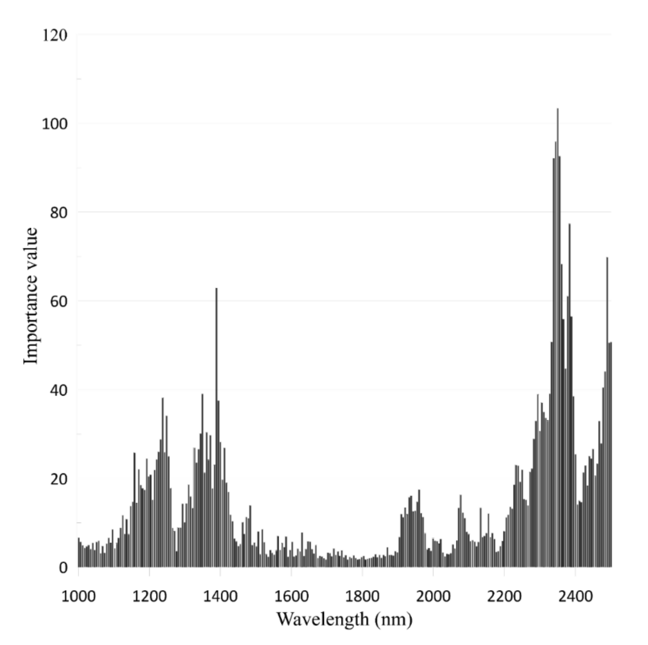
3.1. Band Importance Filtering by Random Forest

This study used band ratio method and logistic regression models to derive simplified open classification models that are applicable in other cases of magnesite exploration based on laboratory hyperspectral approaches. To reduce the number of variables for model construction, a random forest (RF) algorithm was employed to select the best representative bands for magnesite and gangue associated mineral classification. The RF algorithm is a machine learning and ensemble-based model [45,46,47]. Although RF models can do classification and regression as well, one of its useful aspects in addition to the regression function is its ability to rank the variable importance by the Gini index [48]. The Gini index is also called the impurity index. It is used by the decision tree algorithm to select the best variable for splitting the samples. The lowest Gini index represents the most important variable in the classification model. The RF is developed based on a bootstrap sample [45]. The model grows trees from random sampling on the dataset and the variables. The RF model uses 2/3 (known as "in-bag") samples for the training set, and the remaining 1/3 (known as "out-of-bag") for accuracy assessment by cross-validation [45]. The randomly selected subsets of variables are created by user-defined number of features (known as “Mtry”), and the random forest grows to the user-defined number of trees (known as “Ntree”). The final classification is decided based on majority votes from all the trees. Two parameters need to be set in order to produce the forest trees: Ntree and Mtry. In general, the RF classifier can have the maximum number of trees (Ntree) due to its strength of no over-fit. However, we assigned 500 Ntree for this study, as previous studies revealed that the final decision is commonly made before Ntree reaches 500 [49]. The Mtry parameter is set to the square root of the number of input variables [50]. For band selection, we extracted 1000 pixels from each sample image containing information for 269 spectral bands and selected 30 bands derived from the RF model as a by-product for the derivation of band ratios and logistic regression models for the classification of magnesite and associated gangue minerals. We used the SPSS random forest package for band selection.

3.2. Band Ratio

The band ratio is a commonly used multiband image processing method to enhance differences in spectral characteristics and remove environmental biases such as illumination variation and shadows [51,52,53], which has often been used for hyperspectral data classification [54,55]. For selecting the best band radio combination from the 30 bands selected by the RF algorithm, we created a simple band assemblage based on the 30 bands:

$$\mathrm{Y}={{\displaystyle \sum }}_k^{30}\frac{X_k}{X_n}\hspace{1em}(\mathrm{n}=1, 2, 3, ... ,30)$$

(1)

Each band ratio for mineral classes was tested by ANOVA tests, and the tested band combination was further statistically analyzed by the Tamhane T₂ test [56] to compare classification performance among the mineral classes. The band combination with the best classification performance was further analyzed to define index ranges, indicating each class by box plots. The band combination classified carbonate minerals and other types including talc and other types of rock.

3.3. Multi-Variate Logistic Regression

While the band ratio method can select two bands at a time, a multi-variate logistic regression model includes all candidate bands in one model to detect mineral existence. The logistic regression method is a statistical method developed for the analysis and classification of categorical variables [57,58,59]. Therefore, the method is an appropriate approach for detection of a specific mineral [60]. The logistic regression assumes that the occurrence of binary response variable (Y) is controlled by variable (X) and, thus, creates two class plots indicating the event (Y = 1) and no event (Y = 0). The logistic function derives a probability model based on input variables and transforms the probability value to 0 or 1 based on the cut-off value of 0.5 [58,61]. We derived a logistic regression model for each mineral class based on the reflectance value of 30 selected bands from the RF model, following Equations (2) and (3) [62].

$$\mathrm{Logit}{\left(\mathrm{P}\right)}_{\mathrm{mineral}}=\ln \left(\frac{P}{1-P}\right)=\mathrm{C}+{\beta }_1{\mathrm{X}}_1+{\beta }_2{\mathrm{X}}_2+\dots +{\beta }_n{\mathrm{X}}_n$$

(2)

where Logit(P)_mineral indicates the logistic probability of specific mineral occurrence, C is the intercept value, β are the contributions of the covariates to the probability of dependent variable occurrence, and X is the reflectance value of the selected band. Then, the probability of the target event is calculated as

$$P_{\mathrm{mineral}}=\frac{e^{\left(\mathrm{C} +\beta 1\mathrm{X}1+\beta 2\mathrm{X}2 \dots +\beta \mathrm{nXn}\right)}}{1+e^{\left(\mathrm{C} +\beta 1\mathrm{X}1+\beta 2\mathrm{X}2 \dots +\beta \mathrm{nXn}\right)}}$$

(3)

The final p value of a mineral occurrence is assigned as either 1 or 0 based on the 0.5 cut-off value [63]. The logistic regression models developed for each mineral were evaluated by -2 log-likelihood(-2LL) tests and Hosmer and Lemeshow tests. The -2LL evaluates the goodness of fit for the model based on the maximum likelihood regarding the observation and prediction dataset, where a lower value indicates a better fit [64]. The Hosmer and Lemeshow tests evaluate a model based on a log-likelihood ratio between the observation and prediction values, where a model with the highest ratio is considered to have the highest statistical significance [65]. In addition, two coefficients of determination, pseudo-R² values of “Cox and Snell” and “Nagelkerke”, were used to evaluate the logistic regression models [66,67]. The pseudo-R² values are calculated as

$$R^2=1-{\left\{\frac{L\left(M_C\right)}{L\left(M_{\beta }\right)}\right\}}^{\frac{2}{N}} , \mathrm{Cox} \mathrm{and} \mathrm{Snell}$$

(4)

$$R^2=\frac{1-{\left\{\frac{L\left(M_C\right)}{L\left(M_{\beta }\right)}\right\}}^{\frac{2}{N}}}{1-L{\left(M_{\beta }\right)}^{\frac{2}{N}}} , \mathrm{Nagelkerke}$$

(5)

where $L\left(M_C\right)$ is the log-likelihood for a model without explanatory variables, and $L\left(M_{\beta }\right)$ is the log-likelihood for a model with the explanatory variables. Both pseudo-R² values range from 0 to 1, where values closer to 1 indicate better model effectiveness [68]. Moreover, the Wald statistic ((b/standard error)²) was used to evaluate the statistical significance of each explanatory variable [58].

4. Results and Discussion

4.1. Mineral Composition of Mineral Samples Associated with Magnesite

The XRD analysis revealed the mineral composition of the magnesite, dolomite, calcite, and talc samples in this study (

Table 2. The mineral compositions of the samples used in this study.

ID	Origin	Type	Major Mineral	Accessory Mineral
1	Muhak, N.K	Magnesite	Magnesite	Siderite
2	Daehung, N.K	Magnesite	Magnesite, Dolomite, Chlinochlore	Calcite
3	Dashiqiao, C	Magnesite	Magnesite	Dolomite, Talc
4	Muhak, N.K	Magnesite	Magnesite	Quartz
5	Dashiqiao, C	Magnesite	Magnesite	Dolomite
6	Ryongyang, N.K	Magnesite	Magnesite	Chabazite, Calcite
7	Ryongyang, N.K	Magnesite	Magnesite	Dolomite
8	Ryongyang, N.K	Magnesite	Magnesite	Dolomite
9	Ryongyang, N.K	Magnesite	Magnesite	Dolomite
10	Ryongyang, N.K	Magnesite	Magnesite	Dolomite
11	Ryongyang, N.K	Magnesite	Magnesite	Dolomite
12	Ryongyang, N.K	Magnesite	Magnesite
13	Ryongyang, N.K	Magnesite	Magnesite	Dolomite
14	Muhak, N.K	Magnesite	Magnesite	Quartz
15	Ryongyang, N.K	Magnesite	Magnesite
16	Daehung, N.K	Magnesite	Magnesite	Calcite
17	Daehung, N.K	Magnesite	Magnesite
18	Daehung, N.K	Magnesite	Magnesite
19	Daehung, N.K	Magnesite	Magnesite
20	Daehung, N.K	Magnesite	Magnesite	Dolomite
21	Ryongyang, N.K	Magnesite	Magnesite	Dolomite
22	Ryongyang, N.K	Magnesite	Magnesite	Dolomite
23	Daehung, N.K	Magnesite	Magnesite	Dolomite
24	Daehung, N.K	Magnesite	Magnesite	Dolomite
25	Daehung, N.K	Magnesite	Magnesite	Dolomite
26	Daehung, N.K	Magnesite	Magnesite
27	Daehung, N.K	Magnesite	Magnesite
28	Daehung, N.K	Magnesite	Magnesite	Dolomite
29	Sungshin, S.K	Dolomite	Dolomite	Calcite, Magnesite, Quartz
30	Sungshin, S.K	Dolomite	Dolomite, Magnesite	Calcite, Chlinochlore Quartz
31	Dashiqiao, C	Dolomite	Dolomite	Calcite
32	Mungok, S.K	Dolomite	Dolomite	Quartz
33	Mungok, S.K	Dolomite	Dolomite	Quartz
34	Mungok, S.K	Dolomite	Dolomite	Quartz
35	Mungok, S.K	Dolomite	Dolomite
36	Yeongwol, S.K	Dolomite	Dolomite
37	Yeongwol, S.K	Dolomite	Dolomite	Magnesite
38	Jecheon, S.K	Dolomite	Dolomite	Actinolite, Phlogopite
39	Jecheon, S.K	Dolomite	Dolomite	Actinolite, Augite
40	Geomdeog, N.K	Dolomite	Dolomite
41	Geomdeog, N.K	Dolomite	Dolomite
42	Geomdeog, N.K	Dolomite	Dolomite
43	Geomdeog, N.K	Dolomite	Dolomite
44	Geomdeog, N.K	Dolomite	Dolomite
45	Dashiqiao, C	Dolomite	Dolomite	Calcite
46	Sungshin, S.K	Dolomite	Dolomite
47	Sungshin, S.K	Dolomite	Dolomite
48	Sungshin, S.K	Dolomite	Dolomite
49	Sungshin, S.K	Dolomite	Dolomite
50	Mungok, S.K	Dolomite	Dolomite	Quartz
51	Mungok, S.K	Dolomite	Dolomite, Calcite	Quartz
52	Mungok, S.K	Dolomite	Dolomite	Quartz
53	Yeongwol, S.K	Dolomite	Dolomite, Quartz
54	Yeongwol, S.K	Dolomite	Dolomite	Magnesite
55	Yeongwol, S.K	Dolomite	Dolomite	Quartz
56	Yeongwol, S.K	Dolomite	Dolomite
57	Yeongwol, S.K	Dolomite	Dolomite	Magnesite
58	Yeongwol, S.K	Dolomite	Dolomite	Quartz
59	Yeongwol, S.K	Dolomite	Dolomite	Quartz
60	Yeongwol, S.K	Dolomite	Dolomite
61	Jecheon, S.K	Dolomite	Dolomite, Calcite	Magnesite
62	Jecheon, S.K	Dolomite	Dolomite
63	Jecheon, S.K	Dolomite	Dolomite, Calcite
64	Jecheon, S.K	Dolomite	Dolomite, Calcite	Titanite
65	Geomdeog, N.K	Dolomite	Dolomite	Calcite
66	Geomdeog, N.K	Dolomite	Dolomite	Calcite
67	Myeongjin, S.K	Calcite	Calcite	Magnesite, Dolomite
68	Myeongjin, S.K	Calcite	Calcite, Dolomite
69	Myeongjin, S.K	Calcite	Calcite
70	Myeongjin, S.K	Calcite	Calcite, Graphite
71	Myeongjin, S.K	Calcite	Calcite
72	Myeongjin, S.K	Calcite	Calcite
73	Hansol, S.K	Calcite	Calcite	Magnesite
74	Hansol, S.K	Calcite	Calcite
75	Hansol, S.K	Calcite	Calcite	Magnesite
76	Hansol, S.K	Calcite	Calcite	Magnesite
77	Hansol, S.K	Calcite	Calcite
78	Myeongjin, S.K	Calcite	Calcite
79	Myeongjin, S.K	Calcite	Calcite	Magnesite
80	Myeongjin, S.K	Calcite	Calcite, Dolomite
81	Myeongjin, S.K	Calcite	Calcite, Dolomite
82	Sinwol, S.K	Calcite	Calcite, Quartz
83	Sinwol, S.K	Calcite	Calcite	Quartz
84	Sinwol, S.K	Calcite	Calcite	Quartz
85	Sinwol, S.K	Calcite	Calcite	Quartz
86	Sinwol, S.K	Calcite	Calcite, Quartz
87	Sinwol, S.K	Calcite	Calcite
88	Jecheon, S.K	Calcite	Calcite, Magnesite, Dolomite
89	Hansol, S.K	Calcite	Calcite	Magnesite
90	Hansol, S.K	Calcite	Calcite, Magnesite
91	Hansol, S.K	Calcite	Calcite	Magnesite
92	Sinwol, S.K	Calcite	Calcite
93	Sinwol, S.K	Calcite	Calcite
94	Sinwol, S.K	Calcite	Calcite
95	Jecheon, S.K	Calcite	Calcite
96	Geumsan, S,K	Calcite	Calcite	Quartz
97	Dashiqiao, C	Talc	Talc, Calcite	Magnesite
98	Myeongjin, S.K	Talc	Talc
99	Myeongjin, S.K	Talc	Talc
100	Myeongjin, S.K	Talc	Talc, Dolomite
101	Myeongjin, S.K	Talc	Talc
102	Myeongjin, S.K	Talc	Talc, Dolomite
103	Myeongjin, S.K	Talc	Talc, Dolomite
104	Myeongjin, S.K	Talc	Talc, Dolomite
105	Myeongjin, S.K	Talc	Talc, Dolomite
106	Myeongjin, S.K	Talc	Talc
107	Myeongjin, S.K	Talc	Talc, Dolomite
108	Myeongjin, S.K	Talc	Talc, Dolomite
109	Myeongjin, S.K	Talc	Talc
110	Myeongjin, S.K	Talc	Talc
111	Myeongjin, S.K	Talc	Talc, Dolomite
112	Myeongjin, S.K	Talc	Talc
113	Geumsan, S.K	Talc	Talc

). The mineral composition of the magnesite samples from four different origins showed a various combination of accessory minerals. The results confirmed that the natural occurrence of magnesite ore was not pure and was in the form of mineral mixtures. The accessory minerals include dolomite, calcite, chabazite, clinochlore, quartz, and siderite, where dolomite occurred in all magnesite samples. Differently from magnesite samples, dolomite and calcite samples showed significant variations in mineral composition (Table 2), as they are also considered as major rock forming minerals of carbonate rocks. Talc samples contained magnesite, dolomite, and calcite as accessory minerals (Table 2).

Given the fact that carbonate rocks mainly consist of calcite and dolomite and that magnesite mineralization is mainly associated with carbonate rocks with talc as an accessory mineral, pure minerals with a 100% concentration of a specific mineral are rare in field samples. Depending on the involvement of hydrothermal activity, evaporation, replacement, and recrystallization, the compositional combination of calcite, dolomite, magnesite, and talc varies significantly. The results indicate heterogeneous mineral compositions, even for the same types of sample. Because the mineral composition in one type of mineral showed large variations in the mixture of magnesite, dolomite, and calcite, it is highly possible that the spectral information of the spectral library may not be able to detect natural occurrence. Therefore, hyperspectral approaches for magnesite exploration must consider variations in mineral composition for expanded applicability in real-world cases.

4.2. MgO and CaO Content of Magnesite and Dolomite

The major compositional difference between magnesite (MgCO₃) and dolomite (CaMg(CO₃)₂) is mainly determined by Mg and Ca contents, where magnesite rarely contains Ca and dolomite contains low Mg. The chemical composition of magnesite samples from four different locations showed relatively constant MgO and CaO contents (

Table 3. The average MgO and CaO contents of representative magnesite and dolomite samples based on X-ray fluorescence (XRF) analysis.

Location	Type	Number of Samples	MgO	CaO
Muhak, N.K	Magnesite	3	45.5	0.65
Dashiqiao, C	Magnesite	2	47.5	0.79
Ryongyang, N.K	Magnesite	11	47.6	0.73
Daehung, N.K	Magnesite	12	47.4	0.65
Sungshin, S.K	Dolomite	6	13.7	21.0
Mungok, S.K	Dolomite	7	13.8	21.1
Yeongwol, S.K	Dolomite	10	20.8	29.5
Jecheon, S.K	Dolomite	6	20.5	28.8
Geomdeog, N.K	Dolomite	7	21.7	30.8
Dashiqiao, C	Dolomite	2	21.6	30.7

). The MgO content of magnesite samples ranged from 45.5% to 47.6%, with very low CaO content (<0.79%). Compared to magnesite, dolomite samples from six different locations showed larger compositional variation, showing MgO content ranging from 13.7% to 21.7% and CaO content ranging from 21.0% to 30.8% (Table 3). The stoichiometry studies on magnesite revealed that decreases in Ca, Mg, HCO₃, and the Ca/Mg ratio in carbonate fluid (calcite and aragonite) caused magnesite and dolomite mineralization. Dolomite mineralization takes the Ca from the carbonate fluid, resulting in a combination of Mg and Ca contents. Differently from dolomite mineralization, magnesite mineralization occurs at relatively higher temperatures associated with recrystallization, reducing Ca phase replacement in the mineral structure [69]. This result confirms the mineral identification of magnesite and dolomite samples, and variations in Ca composition between the minerals may cause the mineral spectral signature to change. Given the fact that mineral composition and chemical composition are heterogeneous and vary by origin, spectral variation associated with these components accompanies.

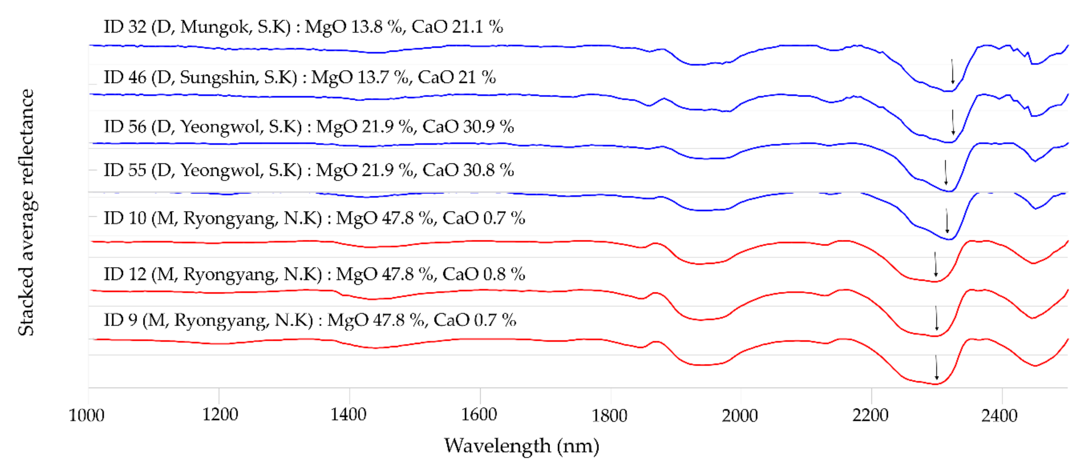
4.3. Spectral Characteristics Associated with Mineral Composition

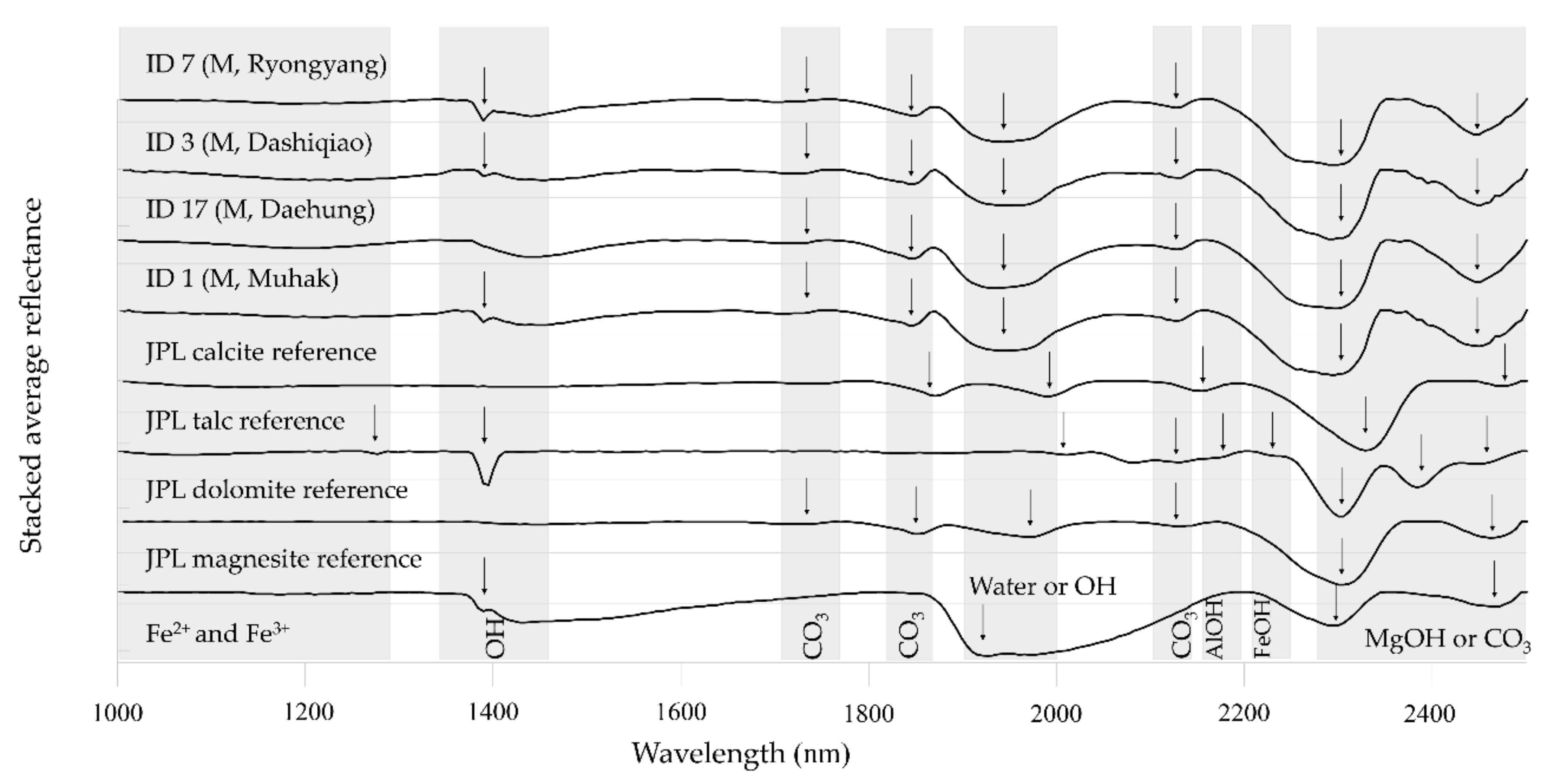
4.3.1. Spectral Characteristics of Magnesite Samples

Spectral analysis on the hull-quoted reflectance spectra of magnesite samples identified strong absorption features at 1850, 1930, 2130, 2300, and 2450 nm, and weak absorption features at 1720 and 2360 nm (Figure 1). Comparing the spectra of magnesite with the JPL (Jet Propulsion Laboratory) reference spectrum, the overlaps in absorption features could only be found at 1389, 1920, 2300, and 2450 nm. The absorption features of the samples at 1720, 1850, and 2130 nm are manifested by dolomite, and that at 2360 nm is affected by calcite and talc.

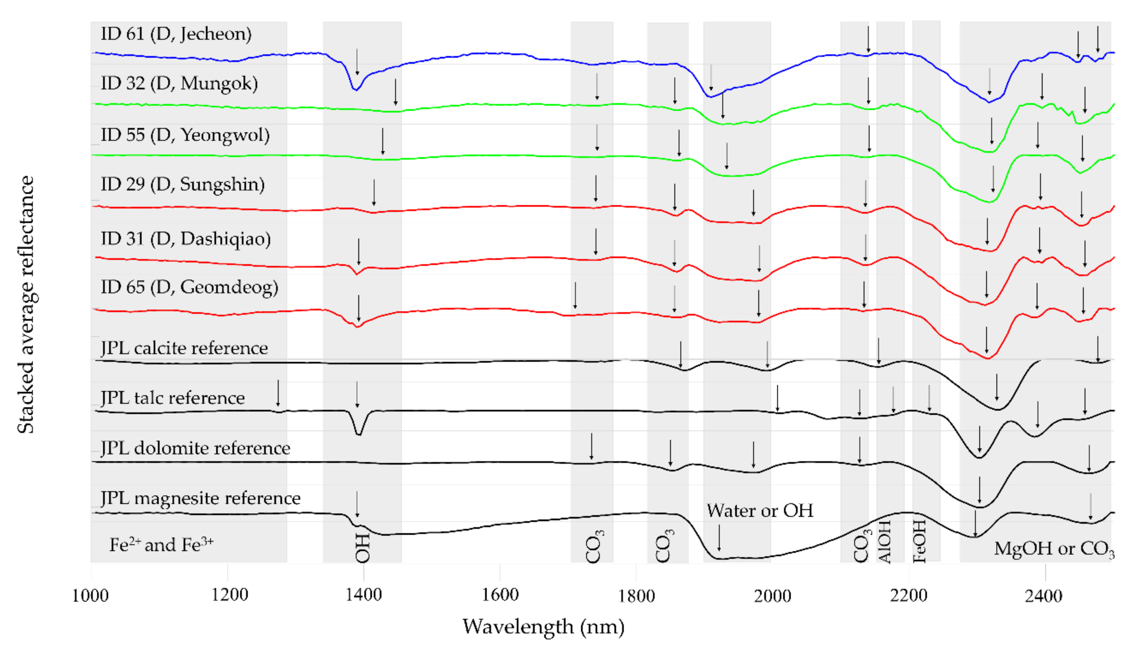
4.3.2. Spectral Characteristics of Dolomite Samples

The spectral characteristics of dolomite can be subdivided to three groups based on mineral composition and absorption features (Figure 2). Comparing the absorption features of the three groups, only two absorptions at 2320 nm of Mg-OH and 2460 nm of CaCO₃ overlaps for all groups. Group 1 includes samples from Sungshin, Geomdeog and Dashiqiao, where calcite accompanies dolomite as a common accessory mineral. The absorption features of group 1 spectra were found at 1860, 2320, and 2460 nm. Group 2 includes samples from Yeongwol and Mungok, where quartz occurs as a common accessory mineral. The absorption features of the group were located at 1900 nm, with additional absorption at 1440 nm, where calcite occurs as an accessory mineral. Group 3 of samples from Jecheon has unique spectral characteristics, showing a smaller number of absorption features and weaker absorptions. The group contains relatively complicated mineral compositions (Table 2). The absorption features were detected at 1389 and 1920 nm of the magnesite signal; at 1720, 2140, and 2320 nm of the dolomite signal; and at 2470 nm of calcite signal. As the results showed, the spectral characteristics of dolomite varied by mineral composition. Comparing the spectral characteristics between magnesite samples and dolomite samples, many absorption features overlap, and the condition is case dependent. It confirms our concern that even when using the hyperspectral images, the magnesite and dolomite samples are hardly separable by simple classification methods and need comprehensive spectral analyses and band selection.

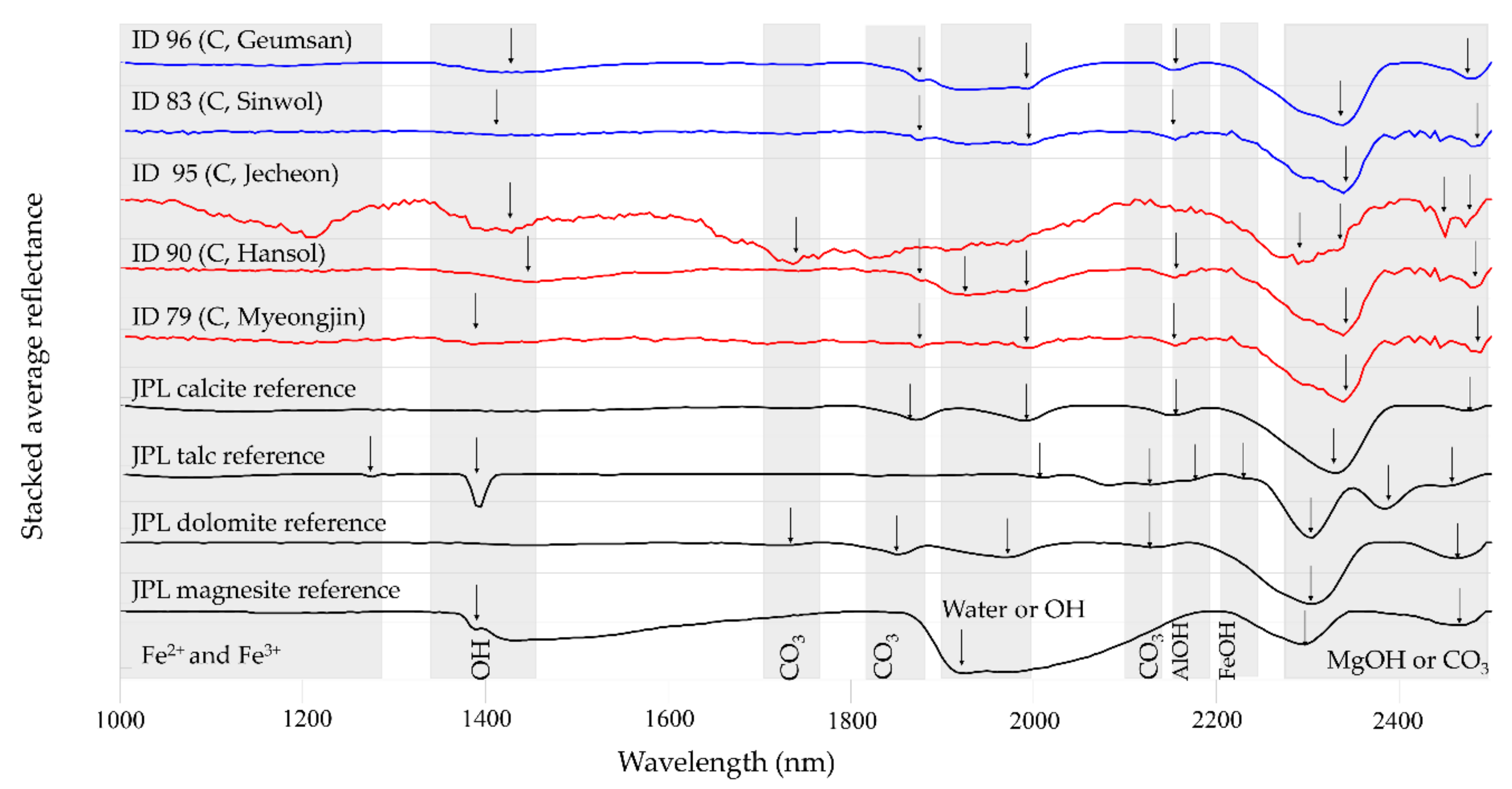
4.3.3. Spectral Characteristics of Calcite Samples

The spectral characteristics of calcite samples can be subdivided to two types. Group 1 includes samples from Myeongjin, Hansol, and Jecheon. The absorption features of group 1 occur at 1394, 1440, 1730, 1920, 2294, 2340, 2470, and 2450 nm, where absorptions at 1440, 2340, and 2470 nm are associated with calcite, and those at 1394, 1920, 2294, and 2450 nm are manifested by magnesite. Additional absorptions of dolomite were found at 1730 nm (Figure 3). These spectral characteristics indicate that they were affected by accessory minerals (Table 2). On the other hand, the spectral curves of group 2 from Sinwol and Geumsan have relatively simple analytical features, where accessory minerals were rarely found. The absorption features of calcite mainly control the spectral characteristics, where absorptions were found at 1411, 1876, 1990, 2160, 2340, and 2470 nm (Figure 3). In the same manner as the other minerals, the calcite samples show large variations in absorption features caused by heterogeneous mineral composition.

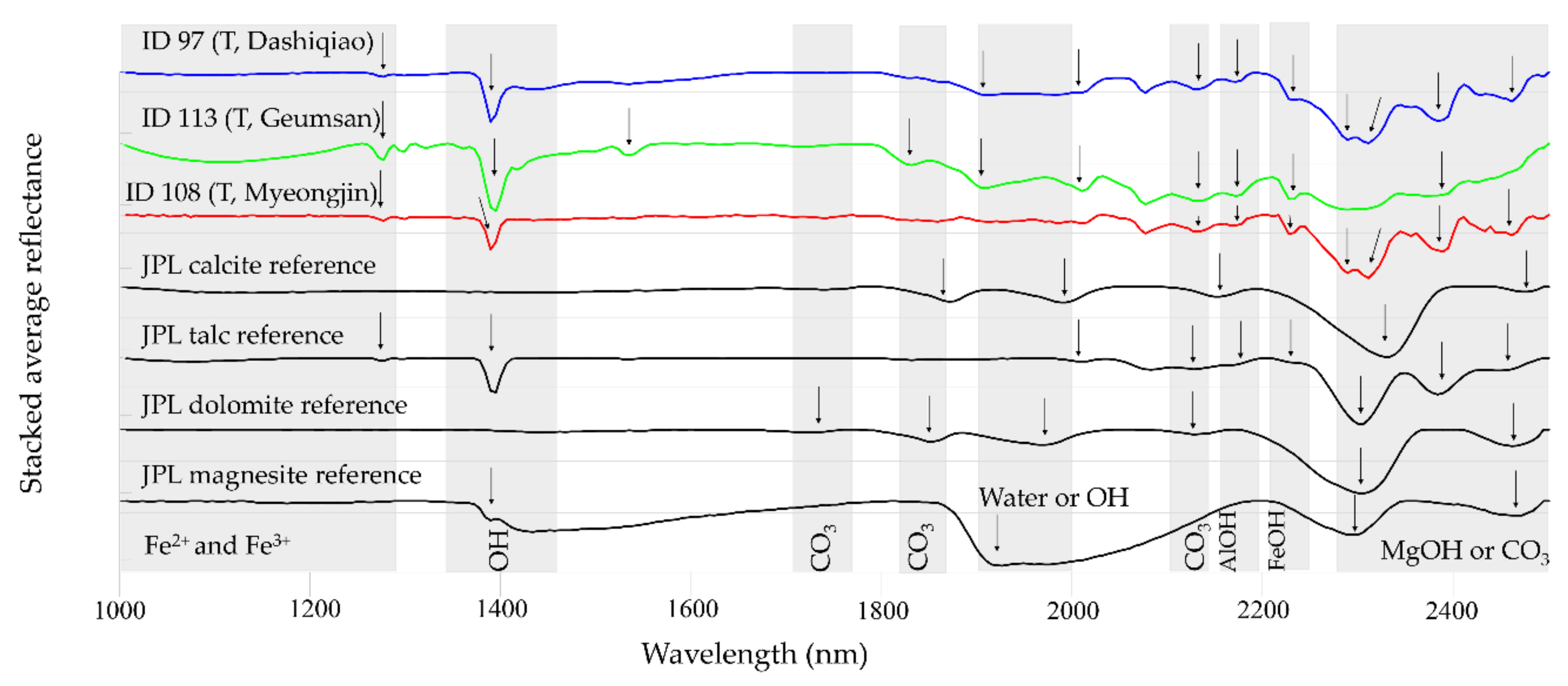
4.3.4. Spectral Characteristics of Talc

Differently from those for other types of mineral, the spectral characteristics of talc samples showed dominant common absorption features at 1276, 1300, 1389, 1910, 2010, 2077, 2133, 2172, 2233, 2290, 2311, and 2383 nm, which were manifested by talc, while minor variation by mineral composition was observed. Group 1 of Myeongjin has talc and dolomite as major minerals, with magnesite as an accessory mineral, showing additional absorption features at 1500, 1800, and 1900 nm. Group 2 of Geumsan shows more distinctive talc spectral features at 1300, 1400, and 1530 nm, where talc is the only major mineral. Group 3 includes samples from Dashiqiao, containing talc and calcite as major minerals and magnesite as an accessory mineral. This group showed additional absorptions of calcite at 1870 nm. These results also confirmed the heterogeneous mineral compositions of naturally formed samples and associated complex variations in spectral curves (Figure 4).

4.3.5. Spectral Characteristics of Magnesite and Dolomite Associated with MgO/CaO Content

To figure out the spectral variations of magnesite and dolomite associated with Mg/Ca content, we analyzed the spectral characteristics of magnesite and dolomite by the MgO/CaO content (Figure 5). It is well known that the absorption feature of Mg-OH around 2300 nm is associated with MgO/CaO content [25,70]. The results showed a systematic shift of the Mg-OH absorption toward a shorter wavelength, with an increase in Mg content regardless of source location. For example, the dolomite spectrum with a MgO content of 13.7% (ID 46) has the maximum absorption at 2322 nm, and that with a MgO content of 21.9 % (ID 55) has the maximum absorption at 2316 nm, showing 6 nm of shift. The maximum absorption feature of Mg-OH for magnesite samples was located at 2294 nm. Compared to the dolomite spectrum of ID 46, the shift of Mg-OH absorption is as much as 28 nm. This study found the same phenomenon from the previous studies for the samples from various source locations [25,70]. It indicates that the shift of Mg-OH absorption is a general phenomenon that may be useful for the detection of Mg content in dolomite and magnesite regardless of source location.

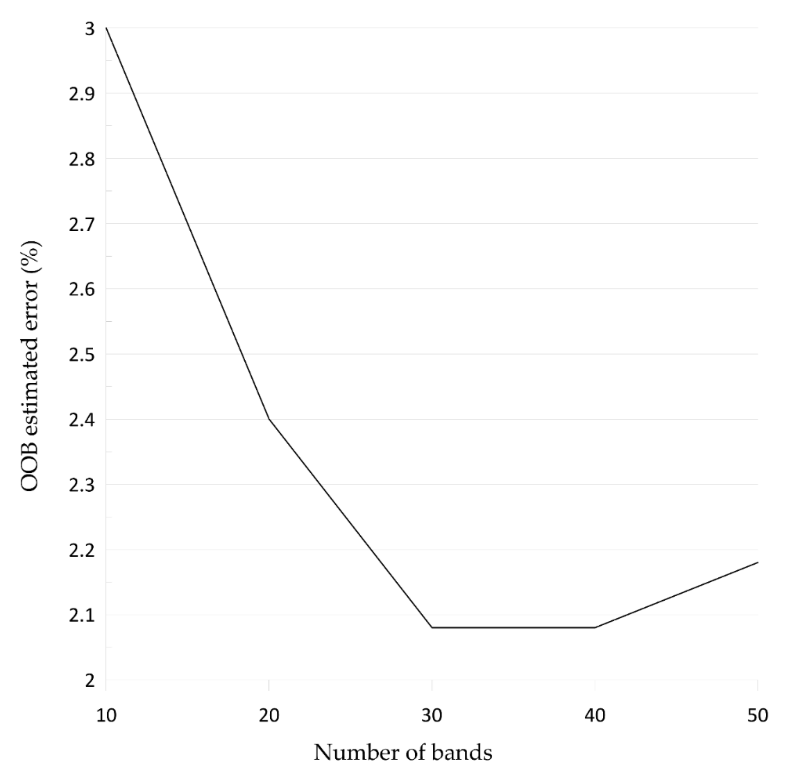
4.4. Band Selection Based on the Random Forest Model

We put the samples into the classification model of a random forest with Ntree = 500 and Mtry = 70. The model returned an overall accuracy of 98.2% (

Table 4. A confusion matrix for the random forest model used for band selection.

Class		Predicted Class (Number of Pixels)
		Magnesite	Dolomite	Talc	Other	Calcite	Accuracy (%)
Actual Class	Magnesite	985	1	4	7	3	98.5
	Dolomite	3	964	2	10	21	99.6
	Talc	0	3	996	0	1	99.6
	Other	0	11	0	981	8	98.1
	Calcite	3	8	0	7	982	98.2
Overall Accuracy							98.2

). The variable importance graph produced from the random forest algorithm (Figure 6) displayed the importance index of all of the input bands. [50] verified that the classification accuracy is superior if a sufficiently higher number of Ntree is used for the small number of variables. The smaller number of variables reduced variable collinearity, and thus could improve a multi-variate regression model. We selected 30 bands for the next step of analysis because, based on Figure 7, the out-of-bag (OOB) error was the lowest near 30 bands. The selected bands were mainly associated with Mg-OH (2289–2384 nm), CO₃ (2467–2500 nm), and OH (1389–1400 nm) (Figure 1 and Figure 6).

Among the 30 selected bands, the highest peak in Figure 6 is near the absorption feature of 2289–2384 nm by Mg-OH. This range has the major absorption features of magnesite, dolomite, calcite, and talc, with a minor shift between the minerals [34,71,72,73]. The second peak in terms of band importance corresponded to carbonate absorptions at 2467–2500nm (magnesite 2450 nm, dolomite/talc 2460 nm, and calcite 2470 nm). Notably, the spectral region showed higher importance than the other absorption features associated with CO₃^2- such as 1750 nm, 1870 nm, 1980 nm, and 2160 nm [36,37,74,75]. The minor shifts of absorption features in the bands between the minerals made the spectral region more effective for classification. The third largest peak comprises of the bands in the range 1389–1394 nm, which is the absorption caused by OH. The spectral bands correspond with the absorption features of magnesite and talc. The selected 30 bands gave an OOB error of less than 1.5% from the RF model (Figure 7). The RF model provides an alternative dimension reduction method for hyperspectral data processing.

4.5. Classification of Magnesite and Associated Gangue Minerals

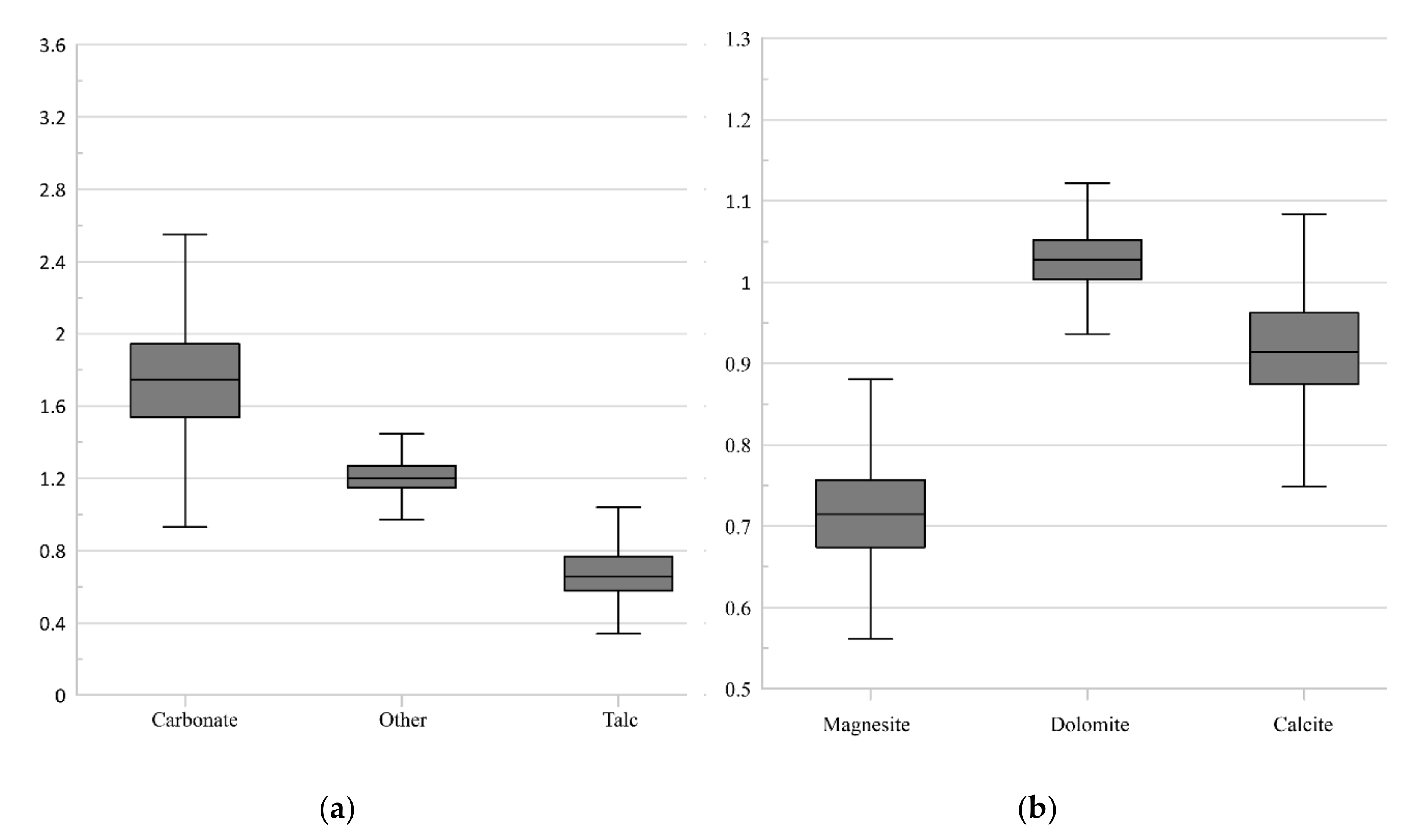
4.5.1. Band Ratio

Based on the combination of 30 selected bands, we derived two band ratio equations, following the band ratio driving method [22]. The band ratio equations were tested for all combinations of band math operations, and the final equations were selected based on Tamhane T₂ and ANOVA tests with the best output results. The first band ratio combination was used to classify carbonate minerals and other types including talc, as Equation (6) below,

$$\mathrm{Y}=\frac{B2328 X B2389}{B2344 X B2483}$$

(6)

where B2328 is the spectral band of 2328 nm, B2344 is the spectral band of 2344 nm, B2389 is the spectral band of 2389 nm, and B2483 is the spectral band of 2483 nm, where the bands of B2328, B2344, and B2483 are related to the absorptions of carbonate minerals and band B2389 corresponds with the absorption shoulder. Then, the second band combination for the classification of carbonate minerals including magnesite, dolomite, and calcite was developed as in Equation (7)

$$\mathrm{Y}=\frac{B2294 X B2355}{B2333 X B2383}$$

(7)

where B2294 is the spectral band of 2294 nm, B2333 is the spectral band of 2333 nm, B2355 is the spectral band of 2355 nm, and B2383 is the spectral band of 2383 nm. B2294 discerns dolomite with higher reflectance than the reflectance of calcite. B2333, B2355, and B2383 show a high reflectance of magnesite and low reflectance of calcite, where absorption locations aligned in order of magnesite, dolomite, and calcite. B2294 is the major absorption band of magnesite, showing a higher reflectance of dolomite.

The classification results based on the band ratios derived above are presented in the box plot (Figure 8) [76]. The first band ratio showed median values for carbonate rock of 1.74, for other types of 1.2, and for talc of 0.65. As shown in Figure 8a, the first band ratio effectively classified carbonate minerals from talc, while the confusion between carbonate minerals and other types was expected. The overall accuracy of the classification was 82% (

Table 5. A confusion matrix for the classification results of carbonate minerals, talc, and other types, by the band ratio method.

Class	Predicted Class (Number of Pixels)
	Talc	Other	Carbonate	Total
Unclassified	3	0	8	11
Talc	0	0	638	638
Other	829	6	42	877
Carbonate	168	994	312	1474
Total	1000	1000	1000	3000
	User’s accuracy (%)		Producer’s accuracy (%)
Talc	94.5		82.9
Other	67.4		99.4
Carbonate	100		63.8
Overall accuracy (%)			82.0

), yet the overall accuracy was acceptable, with the producer’s accuracy for carbonate minerals being 63.9%.

The second band ratio for the discrimination for carbonate minerals showed median values for magnesite of 0.71, calcite of 0.91, and dolomite of 1.02. The range of the index is 0.56–0.88 for magnesite, 0.75–1.08 for calcite, 0.94–1.12 for dolomite (Figure 8b). The overall accuracy of classification for the carbonate minerals was 55.2% (

Table 6. A confusion matrix for the classification results of magnesite, dolomite, and calcite based on the band ratio method.

Class	Predicted Class (Number of Pixels)
	Magnesite	Dolomite	Calcite	Total
Unclassified	0	14	8	22
Magnesite	684	0	28	712
Dolomite	0	25	16	41
Calcite	316	961	948	2225
Total	1000	1000	1000	3000
	User’s accuracy (%)		Producer’s accuracy (%)
Magnesite	96.1		68.4
Dolomite	61.0		02.5
Calcite	42.6		94.8
Overall accuracy (%)			55.2

). However, the classification results for magnesite were acceptable, with a user’s accuracy of 96%.

4.5.2. Binary Logistic Regression Models

To overcome the limitation of the band ratio method and for better generalization, a binary logistic regression model was developed employing the 30 bands selected by the random forest method. Concerning the water bands—namely, the strong absorption wavelengths from water vapor at around 1400 and 1900 nm—because of their low signal to noise ratio [54], we excluded them from the regression model, resulting in 27 bands as the input variables for mineral prediction. Each mineral had one equation developed based on Equation (3) and by a step-wise variable selection mechanism to avoid multicollinearity.

The stepwise variable selection for each target mineral is listed in

Table 7. The final selected variables in the equation and Wald test results from the logistic regression models.

Variable	B1	S.E.2	Wald3	Df4	Sig.5	Exp(B)6
Final selected variables for magnesite classification
B1237 (1237 nm)	44.2	10.237	18.642	1	0	1.57 × 1019
B2294(2294 nm)	−1013.851	235.214	18.579	1	0	0
B2305 (2305 nm)	−1529.829	457.557	11.179	1	0.001	0
B2311 (2311 nm)	1710.024	392.844	18.948	1	0	0
B2316 (2316 nm)	−1645.734	383.517	18.414	1	0	0
B2322 (2322 nm)	1931.354	351.626	30.169	1	0	0
B2361 (2361 nm)	−362.818	88.704	16.73	1	0	0
B2389 (2389 nm)	1629.333	339.902	22.978	1	0	0
B2394 (2394 nm)	−1253.898	306.746	16.71	1	0	0
B2467 (2467 nm)	1211.941	268.864	20.319	1	0	0
B2478 (2478 nm)	−705.467	188.34	14.03	1	0	0
Constant	−11.785	2.24	27.674	1	0	0
Final selected variables for dolomite classification
B1248 (1248 nm)	−44.668	3.422	170.402	1	0	0
B2294 (2294 nm)	289.719	32.46	79.663	1	0	6.66 × 10125
B2316 (2316 nm)	−365.45	51.395	50.561	1	0	0
B2328 (2328 nm)	238.129	63.567	14.033	1	0	2.62 × 10103
B2339 (2339 nm)	−621.411	81.109	58.697	1	0	0
B2344 (2344 nm)	132.733	69.632	3.634	1	0.057	4.42 × 1057
B2355 (2355 nm)	186.986	60.982	9.402	1	0.002	1.61 × 1081
B2361 (2361 nm)	615.639	71.841	73.436	1	0	2.34 × 10267
B2383 (2383 nm)	−334.633	68.317	23.993	1	0	0
B2389 (2389 nm)	−182.19	67.463	7.293	1	0.007	0
B2467 (2467 nm)	346.041	52.612	43.26	1	0	1.92 × 10150
B2483 (2483 nm)	−382.869	79.088	23.436	1	0	0
B2489 (2489 nm)	375.279	86.236	18.938	1	0	9.58 × 10162
B2495 (2495 nm)	−268.606	63.377	17.962	1	0	0
Constant	−1.855	0.203	83.133	1	0	0.157
Final selected variables for calcite classification
B1237 (1237 nm)	−366.642	122.121	9.014	1	0.003	0.000
B1248 (1248 nm)	338.763	121.725	7.745	1	0.005	1.327 × 10147
B2311 (2311 nm)	−2798.173	460.679	36.894	1	0.000	0.000
B2316 (2316 nm)	3090.930	506.840	37.191	1	0.000	0.000
B2339 (2339 nm)	1640.527	312.480	27.563	1	0.000	0.000
B2350 (2350 nm)	−1925.792	462.775	17.317	1	0.000	0.000
B2355 (2355 nm)	−2276.548	479.895	22.504	1	0.000	0.000
B2361 (2361 nm)	2574.915	592.343	18.896	1	0.000	0.000
B2367 (2367 nm)	−1173.638	465.077	6.368	1	0.012	0.000
B2383 (2383 nm)	3050.209	512.796	35.381	1	0.000	0.000
B2394 (2394 nm)	−2088.940	482.653	18.732	1	0.000	0.000
B2467 (2467 nm)	1188.275	342.139	12.062	1	0.001	0.000
B2489 (2489 nm)	−3875.854	731.276	28.091	1	0.000	0.000
B2495 (2495 nm)	3897.919	799.287	23.783	1	0.000	0.000
B2500 (2500 nm)	−1745.837	463.723	14.174	1	0.000	0.000
Constant	0.952	0.842	1.278	1	0.258	2.591
Final selected variables for talc classification
B1237 (1237 nm)	63.06	7.802	65.335	1	0	2.44 × 1027
B2294 (2294 nm)	494.21	133.41	13.723	1	0	4.29 × 10214
B2322 (2322 nm)	−352.872	183.233	3.709	1	0.054	0
B2333 (2333 nm)	−440.763	180.68	5.951	1	0.015	0
B2344 (2344 nm)	763.836	194.177	15.474	1	0	0
B2355 (2355 nm)	−669.464	151.933	19.416	1	0	0
B2372 (2372 nm)	383.697	226.936	2.859	1	0.091	4.34 × 10189
B2383 (2383 nm)	−391.674	143.916	7.407	1	0.006	0
B2467 (2467 nm)	−311.595	204.861	2.313	1	0.128	0
B2478 (2478 nm)	435.462	262.939	2.743	1	0.098	1.32 × 10189
B2495 (2495 nm)	468.646	291.343	2.587	1	0.108	3.39 × 10203
B2500 (2500 nm)	−544.645	219.341	6.166	1	0.013	0
Constant	−6.352	1.213	27.417	1	0	0.002

B¹ = logistic coefficient; S.E.² = standard error of estimate; Wald³ = Wald chi-square values; Df⁴ = degree of freedom; Sig.⁵ = P-value; Exp(B)⁶ = exponentiated coefficient

. The classification equation for magnesite employed 11 variables, among which eight bands are associated with Mg-OH spectral features, two bands are from Ca features, and one band is at 1237 nm (Table 7). For dolomite, the equation was developed based on nine bands from Mg-OH features, four bands from Ca features, and one band at 1248 nm (Table 7). Differently from magnesite, seven bands were significant, and the most important bands were 2361 and 2489 nm of Mg-OH features. The calcite equation was derived from nine bands from Mg-OH features and four bands from Ca features, along with bands at 1237 and 1248 nm. The band at 1248 nm plays an important role in calcite detection. Talc classification was based on seven bands of Mg-OH features, four bands of Ca features, and the band at 1237 nm (Table 7), where Mg-OH bands play important roles.

All logistic regression equations employed the band at 2467 nm, and three models employed the bands at 1237, 2294, 2316, 2355, 2361, and 2495 nm. The absorption features associated with Mg-OH and Ca participated in all regression equations, where the absorption depth, peak absorption, and absorption width vary among the target minerals. Exceptionally, the spectral band of 1237 nm participated in three regression models, even though the band has no absorption feature. The spectral signatures (1200 nm range) of the minerals show consistent low standard errors (Table 7). Indeed, [77] also used spectral features other than the 2000–2300 nm region for the detection and classification of carbonatites among sedimentary carbonates. Moreover, the RF algorithm identified 1200 nm as important spectral bands for the classification of target minerals. The overall accuracy of the classification was 99.9% for magnesite, 98% for dolomite, 99.6% for calcite, and 99.8% for talc (

Table 8. An accuracy table for the classification results derived from binary logistic regression models.

		Predicted (Number of Pixels)		Correct Percentage
Observed		No Event (0)	Event (1)
Magnesite	0	3999	1	100
	1	5	995	99.5
Overall Percentage				99.9
Dolomite	0	3975	25	99.4
	1	77	923	92.3
Overall Percentage				98.0
Calcite	0	3991	9	99.8
	1	7	993	99.3
Overall Percentage				99.7
Talc	0	3995	5	99.9
	1	5	995	99.5
Overall Percentage				99.8

).

Evaluation of Binary Regression Models

The results of Hosmer and Lemeshow test showed that the p values of the X² values of the logistic regression models for the target minerals range from 0.472 for dolomite to 0.997 for magnesite and calcite (

Table 9. The statistical parameters of the logistic regression models.

Statistical Parameters	Hosmer and Lemeshow Test			Pseudo-R2
	X2	df	P Value	Cox & Snell R2	Nagelkerke R2
Magnesite	1.180	8	0.997	0.628	0.994
Dolomite	7.613	8	0.472	0.580	0.917
Calcite	1.129	8	0.997	0.625	0.988
Talc	1.425	8	0.994	0.626	0.989

). In general, significance higher than 0.05 is acceptable, and the test showed that all models are statistically coherent [64].

In addition, the goodness of fit was tested based on pseudo-R², where pseudo-R² ranged from 0.58 to 0.628 for Cox & Snell R², and 0.917 to 0.994 for Nagelkerke R² (Table 9). In general, Cox & Snell pseudo-R² values larger than 0.2 are considered to indicate good fit [78]. The psuedo-R² values of the models validated that all models have a strong goodness of fit.

Validation of Binary Regression Models

The binary regression models for detection of magnesite, dolomite, calcite, and talc developed from training samples were applied to 46 validation samples (Figure 9). The accuracy of the magnesite logistic regression model was 97.6%. All magnesite samples were correctly detected, while some pixels of magnesite samples were classified as none (Figure 9a and

Table 10. A confusion matrix for the classification results of the validation set from the binary regression models.

Class	Correct class		Non correct class		Overall accuracy (%)
	Producer’s accuracy (%)	User’s accuracy (%)	Producer’s accuracy (%)	User’s accuracy (%)
Magnesite	99.7	95.6	95.6	99.7	97.6
Dolomite	54.4	99.3	77.3	99.8	82
Calcite	47.6	71.1	95.9	98.4	94.6
Talc	99.5	92.31	99.8	99.9	99.8

). The overall accuracy of the dolomite model was 82%, where the model classified 9 out of 21 dolomite samples (Figure 9b and Table 10). The accuracy of dolomite was lower than of the other minerals. The erroneous samples include calcite and/or quartz as major minerals (Table 2). The bias might be caused by the mix of major spectra manifested by both minerals. The calcite model classified 94.6% of calcite pixels correctly (Figure 9c and Table 10). The accuracy of the talc model was very high (99.8%, Figure 9d and Table 10).

4.6. Discussions and Limitations of the Present Work

Based on the classification results applied to the validation samples, the logistic regression models showed significantly higher accuracy than the band ratio method. While the band ratio method is easier to apply, its overall accuracy was about 40% lower than that of the logistic regression models for carbonate mineral classification. In addition, we compared the effectiveness of the logistic regression models with the RF method. The classification results of the RF method for the validation samples showed an accuracy ranging from 92.6% to 99.9%, with an overall accuracy of 96.6% (

Table 11. A confusion matrix for the classification results of the validation set from the random forest algorithm.

Class		Predicted Class (Number of Pixels)
		Magnesite	Dolomite	Talc	Calcite	Accuracy (%)
Actual Class	Magnesite	997	3	0	0	99.7
	Dolomite	2	926	0	72	92.6
	Talc	0	0	999	1	99.9
	Calcite	0	56	0	944	94.4
Overall Accuracy (%)						96.6

). The accuracy of the RF method was similar with the logistic regression models except for the dolomite samples. The RF method showed better performance on dolomite classification, with 92.6%. Although the RF method shows a slightly better accuracy, the knowledge learned by the RF algorithm is wrapped in its complex data structure as a black box to the researchers. On the contrary, the logistic models have simple form and can be easily generalized to other case studies for magnesite exploration.

Given the fact that this study developed the models using naturally occurring samples from various locations and that the mineral composition is heterogeneous, the models tested in this study could be applicable for real-world cases as prompt analytical methods for sample discrimination. Analysts can select the best model for their case studies. For hyperspectral band surveys, we recommend the logistic regression model.

Although our study is comprehensive on the band selection, the target minerals only include four major ones. It is not difficult to conclude that if more minerals are considered, the complexity of the prediction model will drastically increase. Furthermore, this study is based on fresh samples with controlled dry conditions. The weathering process and wet surface would complicate the spectral signals associated with hydrolysis and water components [38,79]. Adding controlled moisture and weathered samples would allow us to better understand the uncertainty in mapping magnesite in a natural environment. The band selection and band-ratio equations will be different under different assumptions of surface moisture and weathering. Our research proved the feasibility of the method we developed for fresh dry samples and could serve a role model for these future case studies.

5. Conclusions

This study introduced a detection method for magnesite and associated gangue minerals including dolomite, calcite, and talc based on mineralogical, chemical, and hyperspectral analyses using SWIR hyperspectral images under laboratory conditions. The samples used for this study originated from thirteen different locations in South Korea, China, and North Korea and were used to develop detection models with wide applicability. The spectral characteristics of sample spectra were analyzed with consideration of minerals and composition. Using the spectral characteristics derived from the hyperspectral images, the random forest algorithm was used for band selection and dimension reduction. Band ratio and logistic regression models were developed to find the most useful detection methods.

The mineralogical analysis revealed the heterogeneity of mineral composition for naturally occurring samples. Magnesite samples contains accessory minerals such as dolomite, calcite, chabazite, clinochlore, quartz, and siderite. Dolomite and calcite samples showed the accessory minerals actinolite, augite, calcite, graphite, magnesite, phlogopite, quartz, and titanite. Talc samples had magnesite, dolomite, and calcite as accessory minerals. The results indicate the heterogeneity of mineral composition, even for the same types of sample. Because the mineral composition in one type of mineral showed large variations—mainly mixed forms of magnesite, dolomite, and calcite—the hyperspectral approaches for magnesite exploration must consider variations in mineral composition in other case studies. The Mg and Ca composition of magnesite and dolomite varied significantly, where magnesite had more Mg content and dolomite had more Ca content. These results confirmed the heterogeneity of minerals in not only the mineral composition but also the chemical composition of major elements.

The spectral characteristics of the magnesite samples were found at the absorption features located at 1850, 1930, 2130, 2300, and 2450 nm, with weak absorptions at 1720 and 2360 nm. The spectral characteristics represent the heterogeneity of mineral composition, where absorption features of dolomite, calcite, and talc were found in the spectra of magnesite samples. The same phenomenon was found for dolomite, calcite, and talc samples, where major absorptions of each mineral were mixed with other minerals’ absorptions from the sample spectra, representing heterogeneous mineral composition. The spectral characteristics of magnesite and dolomite showed systematic variations in Mg-OH absorption features toward a shorter wavelength, with an increase in Mg content. This indicates that the shift of Mg-OH absorption may be useful for the detection of Mg content in dolomite and magnesite.

The random forest algorithm reduced the number of bands by selecting 30 of the most sensitive bands for the classification of magnesite and associated gangue minerals. The selected bands were mainly associated with Mg-OH (2289–2384 nm), CO₃ (2467–2500 nm), and OH (1389–1400 nm). Among the selected bands, the bands with the highest importance were found in spectral range of Mg-OH absorptions, followed by the spectral bands around carbonate and hydrolysis absorptions. A two-step band ratio method was derived using the selected bands. The first step classified carbonate minerals from talc and other types of sample with an accuracy of 92%. The second step classified magnesite, dolomite, and calcite with an accuracy of 55.2%, where the classification results were not satisfactory. The logistic regression models based on the 27 selected bands excluding water bands achieved accuracies of 98%~99.9% for the training samples and 82–99.8% for the validation samples.

Given the fact that this study found the naturally formed samples from various locations showing heterogeneous mineral composition, the applicability of the models would expand to general use as a prompt analytical method for sample discrimination. It is necessary to include more samples with more source locations to refine and enhance the model. Furthermore, the method would expand its applicability to carbonate rocks and minerals exploration significantly if the method was tested in the field.

References

1. Salazar, K. Mineral Commodity Summaries 2013: US Geological Survey (USGS). US Geol. Surv. 2013. [Google Scholar] [CrossRef]
2. Park, H.-K.; Park, J.-T.; Lee, H.-I.; Choi, Y.-Y. Characteristics in Calcination of Magnesite Ore in Yongyang Mines. J. Korean Inst. Resour. Recycl. 2005, 14, 33–38. [Google Scholar]
3. Sibanda, Z.; Amponsah-Dacosta, F.; Mhlongo, S. Characterization and evaluation of magnesite tailings for their potential utilization: A case study of nyala magnesite mine, limpopo province of South Africa. ARPN J. Eng. Appl. Sci. 2013, 8, 606–613. [Google Scholar]
4. Melezhik, V.A.; Fallick, A.E.; Medvedev, P.V.; Makarikhin, V.V. Palaeoproterozoic magnesite: Lithological and isotopic evidence for playa/sabkha environments. Sedimentology 2001, 48, 379–397. [Google Scholar] [CrossRef]
5. Lippmann, F. Sedimentary Carbonate Minerals; Springer Science & Business Media: Heidelberg, Germany, 2012; Volume 6. [Google Scholar]
6. Machel, H.G. Concepts and models of dolomitization: A critical reappraisal. Geol. Soc. Lond. Spec. Publ. 2004, 235, 7–63. [Google Scholar] [CrossRef]
7. Pohl, W. Comparative geology of magnesite deposits and occurrences. Magnesite Geol. Mineral. Geochem. Form. Mg-Carbonates 1989, 28, 1–13. [Google Scholar]
8. Pohl, W. Genesis of magnesite deposits—Models and trends. Geol. Rundsch. 1990, 79, 291–299. [Google Scholar] [CrossRef]
9. Warren, J. Dolomite: Occurrence, evolution and economically important associations. Earth Sci. Rev. 2000, 52, 1–81. [Google Scholar] [CrossRef]
10. Baldermann, A.; Deditius, A.P.; Dietzel, M.; Fichtner, V.; Fischer, C.; Hippler, D.; Leis, A.; Baldermann, C.; Mavromatis, V.; Stickler, C.P. The role of bacterial sulfate reduction during dolomite precipitation: Implications from Upper Jurassic platform carbonates. Chem. Geol. 2015, 412, 1–14. [Google Scholar] [CrossRef]
11. Given, R.K.; Wilkinson, B.H. Dolomite abundance and stratigraphic age; constraints on rates and mechanisms of Phanerozoic dolostone formation. J. Sediment. Res. 1987, 57, 1068–1078. [Google Scholar] [CrossRef]
12. Budd, D. Cenozoic dolomites of carbonate islands: Their attributes and origin. Earth Sci. Rev. 1997, 42, 1–47. [Google Scholar] [CrossRef]
13. Prochaska, W. Genetic concepts on the formation of the Austrian magnesite and siderite mineralizations in the Eastern Alps of Austria. Geol. Croat. 2016, 69, 31–38. [Google Scholar] [CrossRef] [Green Version]
14. Misch, D.; Pluch, H.; Mali, H.; Ebner, F.; Huang, H. Genesis of giant Early Proterozoic magnesite and related talc deposits in the Mafeng area, Liaoning Province, NE China. J. Asian Earth Sci. 2018, 160, 1–12. [Google Scholar] [CrossRef]
15. Neubauer, F. Structural Control on the Formation of Ttalc Deposits; Balkeema Publ.: Lassing, Austria, 2001. [Google Scholar]
16. Railsback, L.B. Patterns in the compositions, properties, and geochemistry of carbonate minerals. Carbonates Evaporites 1999, 14, 1. [Google Scholar] [CrossRef]
17. Tangestani, M.H.; Moore, F. Iron oxide and hydroxyl enhancement using the Crosta Method: A case study from the Zagros Belt, Fars Province, Iran. Int. J. Appl. Earth Obs. Geoinf. 2000, 2, 140–146. [Google Scholar] [CrossRef]
18. Yip, C.K.; Provis, J.L.; Lukey, G.C.; van Deventer, J.S. Carbonate mineral addition to metakaolin-based geopolymers. Cem. Concr. Compos. 2008, 30, 979–985. [Google Scholar] [CrossRef]
19. Friedman, G.M. Identification of carbonate minerals by staining methods. J. Sediment. Res. 1959, 29, 87–97. [Google Scholar] [CrossRef]
20. Dickson, J. Carbonate identification and genesis as revealed by staining. J. Sediment. Res. 1966, 36, 491–505. [Google Scholar] [CrossRef]
21. Laakso, K.; Middleton, M.; Heinig, T.; Bärs, R.; Lintinen, P. Assessing the ability to combine hyperspectral imaging (HSI) data with Mineral Liberation Analyzer (MLA) data to characterize phosphate rocks. Int. J. Appl. Earth Obs. Geoinf. 2018, 69, 1–12. [Google Scholar] [CrossRef]
22. Rajendran, S.; Hersi, O.S.; Al-Harthy, A.; Al-Wardi, M.; El-Ghali, M.A.; Al-Abri, A.H. Capability of advanced spaceborne thermal emission and reflection radiometer (ASTER) on discrimination of carbonates and associated rocks and mineral identification of eastern mountain region (Saih Hatat window) of Sultanate of Oman. Carbonates Evaporites 2011, 26, 351–364. [Google Scholar] [CrossRef]
23. Rajendran, S.; Nasir, S. ASTER spectral analysis of ultramafic lamprophyres (carbonatites and aillikites) within the Batain Nappe, northeastern margin of Oman: A proposal developed for spectral absorption. Int. J. Remote Sens. 2013, 34, 2763–2795. [Google Scholar] [CrossRef]
24. Rajendran, S.; Nasir, S.; Kusky, T.M.; Ghulam, A.; Gabr, S.; El-Ghali, M.A. Detection of hydrothermal mineralized zones associated with listwaenites in Central Oman using ASTER data. Ore Geol. Rev. 2013, 53, 470–488. [Google Scholar] [CrossRef]
25. Mars, J.C.; Rowan, L.C. Spectral assessment of new ASTER SWIR surface reflectance data products for spectroscopic mapping of rocks and minerals. Remote Sens. Environ. 2010, 114, 2011–2025. [Google Scholar] [CrossRef]
26. Amer, R.; Kusky, T.; Ghulam, A. Lithological mapping in the Central Eastern Desert of Egypt using ASTER data. J. Afr. Earth Sci. 2010, 56, 75–82. [Google Scholar] [CrossRef]
27. Gabr, S.; Ghulam, A.; Kusky, T. Detecting areas of high-potential gold mineralization using ASTER data. Ore Geol. Rev. 2010, 38, 59–69. [Google Scholar] [CrossRef]
28. Kruse, F.A.; Boardman, J.W.; Huntington, J.F. Comparison of airborne hyperspectral data and EO-1 Hyperion for mineral mapping. IEEE Trans. Geosci. Remote Sens. 2003, 41, 1388–1400. [Google Scholar] [CrossRef] [Green Version]
29. Kodikara, G.R.; Woldai, T.; van Ruitenbeek, F.J.; Kuria, Z.; van der Meer, F.; Shepherd, K.D.; Van Hummel, G. Hyperspectral remote sensing of evaporate minerals and associated sediments in Lake Magadi area, Kenya. Int. J. Appl. Earth Obs. Geoinf. 2012, 14, 22–32. [Google Scholar] [CrossRef]
30. Govil, H.; Gill, N.; Rajendran, S.; Santosh, M.; Kumar, S. Identification of new base metal mineralization in Kumaon Himalaya, India, using hyperspectral remote sensing and hydrothermal alteration. ORE Geol. Rev. 2018, 92, 271–283. [Google Scholar] [CrossRef]
31. Jain, R.; Sharma, R.U. Airborne hyperspectral data for mineral mapping in Southeastern Rajasthan, India. Int. J. Appl. Earth Obs. Geoinf. 2019, 81, 137–145. [Google Scholar] [CrossRef]
32. Carrino, T.A.; Crósta, A.P.; Toledo, C.L.B.; Silva, A.M. Hyperspectral remote sensing applied to mineral exploration in southern Peru: A multiple data integration approach in the Chapi Chiara gold prospect. Int. J. Appl. Earth Obs. Geoinf. 2018, 64, 287–300. [Google Scholar] [CrossRef]
33. Krupnik, D.; Khan, S.; Okyay, U.; Hartzell, P.; Zhou, H.-W. Study of Upper Albian rudist buildups in the Edwards Formation using ground-based hyperspectral imaging and terrestrial laser scanning. Sediment. Geol. 2016, 345, 154–167. [Google Scholar] [CrossRef] [Green Version]
34. Baissa, R.; Labbassi, K.; Launeau, P.; Gaudin, A.; Ouajhain, B. Using HySpex SWIR-320m hyperspectral data for the identification and mapping of minerals in hand specimens of carbonate rocks from the Ankloute Formation (Agadir Basin, Western Morocco). J. Afr. Earth Sci. 2011, 61, 1–9. [Google Scholar] [CrossRef]
35. Zaini, N.; Van der Meer, F.; Van der Werff, H. Determination of carbonate rock chemistry using laboratory-based hyperspectral imagery. Remote Sens. 2014, 6, 4149–4172. [Google Scholar] [CrossRef] [Green Version]
36. Hunt, G.R.; Salisbury, J.W. Visible and near infrared spectra of minerals and rocks. II. Carbonates. Mod. Geol. 1971, 2, 23–30. [Google Scholar]
37. Gaffey, S.J. Spectral reflectance of carbonate minerals in the visible and near infrared (0.35-2.55 microns); calcite, aragonite, and dolomite. Am. Mineral. 1986, 71, 151–162. [Google Scholar]
38. Shin, J.H.; Yu, J.; Wang, L.; Kim, J.; Koh, S.-M.; Kim, S.-O. Spectral responses of heavy metal contaminated soils in the vicinity of a hydrothermal ore deposit: A case study of Boksu Mine, South Korea. IEEE Trans. Geosci. Remote Sens. 2019, 57, 4092–4106. [Google Scholar] [CrossRef]
39. Quinn, T. About Magforum. 2017; ISSN 1756-364X. [Google Scholar]
40. Kruse, F.A.; Bedell, R.L.; Taranik, J.V.; Peppin, W.A.; Weatherbee, O.; Calvin, W.M. Mapping alteration minerals at prospect, outcrop and drill core scales using imaging spectrometry. Int. J. Remote Sens. 2012, 33, 1780–1798. [Google Scholar] [CrossRef] [Green Version]
41. Smith, G.M.; Milton, E.J. The use of the empirical line method to calibrate remotely sensed data to reflectance. Int. J. Remote Sens. 1999, 20, 2653–2662. [Google Scholar] [CrossRef]
42. Green, A.A.; Berman, M.; Switzer, P.; Craig, M.D. A transformation for ordering multispectral data in terms of image quality with implications for noise removal. IEEE Trans. Geosci. Remote Sens. 1988, 26, 65–74. [Google Scholar] [CrossRef] [Green Version]
43. Shawky, M.M.; El-Arafy, R.A.; El Zalaky, M.A.; Elarif, T. Validating (MNF) transform to determine the least inherent dimensionality of ASTER image data of some uranium localities at Central Eastern Desert, Egypt. J. Afr. Earth Sci. 2019, 149, 441–450. [Google Scholar] [CrossRef]
44. Kokaly, R.F.; Clark, R.N. Spectroscopic determination of leaf biochemistry using band-depth analysis of absorption features and stepwise multiple linear regression. Remote Sens. Environ. 1999, 67, 267–287. [Google Scholar] [CrossRef]
45. Breiman, L. Random forests. Mach. Learn. 2001, 45, 5–32. [Google Scholar] [CrossRef] [Green Version]
46. Guo, L.; Chehata, N.; Mallet, C.; Boukir, S. Relevance of airborne lidar and multispectral image data for urban scene classification using Random Forests. ISPRS J. Photogramm. Remote Sens. 2011, 66, 56–66. [Google Scholar] [CrossRef]
47. Rodriguez-Galiano, V.F.; Ghimire, B.; Rogan, J.; Chica-Olmo, M.; Rigol-Sanchez, J.P. An assessment of the effectiveness of a random forest classifier for land-cover classification. ISPRS J. Photogramm. Remote Sens. 2012, 67, 93–104. [Google Scholar] [CrossRef]
48. Abdel-Rahman, E.M.; Mutanga, O.; Adam, E.; Ismail, R. Detecting Sirex noctilio grey-attacked and lightning-struck pine trees using airborne hyperspectral data, random forest and support vector machines classifiers. ISPRS J. Photogramm. Remote Sens. 2014, 88, 48–59. [Google Scholar] [CrossRef]
49. Lawrence, R.L.; Wood, S.D.; Sheley, R.L. Mapping invasive plants using hyperspectral imagery and Breiman Cutler classifications (RandomForest). Remote Sens. Environ. 2006, 100, 356–362. [Google Scholar] [CrossRef]
50. Gislason, P.O.; Benediktsson, J.A.; Sveinsson, J.R. Random forests for land cover classification. Pattern Recognit. Lett. 2006, 27, 294–300. [Google Scholar] [CrossRef]
51. Kim, M.S.; Chen, Y.-R.; Cho, B.-K.; Chao, K.; Yang, C.-C.; Lefcourt, A.M.; Chan, D. Hyperspectral reflectance and fluorescence line-scan imaging for online defect and fecal contamination inspection of apples. Sens. Instrum. Food Qual. Saf. 2007, 1, 151. [Google Scholar] [CrossRef]
52. Ninomiya, Y.; Fu, B.; Cudahy, T.J. Detecting lithology with Advanced Spaceborne Thermal Emission and Reflection Radiometer (ASTER) multispectral thermal infrared “radiance-at-sensor” data. Remote Sens. Environ. 2005, 99, 127–139. [Google Scholar] [CrossRef]
53. Rajendran, S.; Al-Khirbash, S.; Pracejus, B.; Nasir, S.; Al-Abri, A.H.; Kusky, T.M.; Ghulam, A. ASTER detection of chromite bearing mineralized zones in Semail Ophiolite Massifs of the northern Oman Mountains: Exploration strategy. ORE Geol. Rev. 2012, 44, 121–135. [Google Scholar] [CrossRef]
54. Kurz, T.H.; Dewit, J.; Buckley, S.J.; Thurmond, J.B.; Hunt, D.W.; Swennen, R. Hyperspectral image analysis of different carbonate lithologies (limestone, karst and hydrothermal dolomites): The Pozalagua Quarry case study (Cantabria, North-west Spain). Sedimentology 2012, 59, 623–645. [Google Scholar] [CrossRef]
55. Gad, S.; Kusky, T. ASTER spectral ratioing for lithological mapping in the Arabian–Nubian shield, the Neoproterozoic Wadi Kid area, Sinai, Egypt. Gondwana Res. 2007, 11, 326–335. [Google Scholar] [CrossRef]
56. Kay, D.; Crowther, J.; Stapleton, C.M.; Wyer, M.D.; Fewtrell, L.; Edwards, A.; Francis, C.; McDonald, A.T.; Watkins, J.; Wilkinson, J. Faecal indicator organism concentrations in sewage and treated effluents. Water Res. 2008, 42, 442–454. [Google Scholar] [CrossRef] [PubMed]
57. Agresti, A. Categorical Data Analysis. John Wiley & Sons: Hoboken, NJ, USA, 2003; Volume 482. [Google Scholar]
58. Hair, J.F.; Black, W.C.; Babin, B.J.; Anderson, R.E.; Tatham, R.L. Multivariate Data Analysis; Pearson Prentice Hall: Upper Saddle River, NJ, USA, 2006; Volume 6. [Google Scholar]
59. Pohar, M.; Blas, M.; Turk, S. Comparison of logistic regression and linear discriminant analysis: A simulation study. Metodoloski Zv. 2004, 1, 143. [Google Scholar]
60. Yousefi, M.; Carranza, E.J.M. Prediction–area (P–A) plot and C–A fractal analysis to classify and evaluate evidential maps for mineral prospectivity modeling. Comput. Geosci. 2015, 79, 69–81. [Google Scholar] [CrossRef]
61. Bewick, V.; Cheek, L.; Ball, J. Statistics review 14: Logistic regression. Crit. Care 2005, 9, 112. [Google Scholar] [CrossRef] [Green Version]
62. Hosmer Jr, D.W.; Lemeshow, S.; Sturdivant, R.X. Applied Logistic Regression; John Wiley & Sons: New Jersey, NJ, USA, 2013; Volume 398. [Google Scholar]
63. Sahoo, N.R.; Pandalai, H.S. Integration of Sparse Geologic Information in Gold Targeting Using Logistic Regression Analysis in the Hutti–Maski Schist Belt, Raichur, Karnataka, India—A Case Study. Nat. Resour. Res. 1999, 8, 233–250. [Google Scholar] [CrossRef]
64. Mokhtari, A.R. Hydrothermal alteration mapping through multivariate logistic regression analysis of lithogeochemical data. J. Geochem. Explor. 2014, 145, 207–212. [Google Scholar] [CrossRef]
65. Hosmer, D.W.; Lemeshow, S. Applied Logistic Regression; John Wiley & Sons,: New York, NJ, USA, 1989. [Google Scholar]
66. Menard, S. Coefficients of determination for multiple logistic regression analysis. Am. Stat. 2000, 54, 17–24. [Google Scholar]
67. Nagelkerke, N.J. A note on a general definition of the coefficient of determination. Biometrika 1991, 78, 691–692. [Google Scholar] [CrossRef]
68. Ayalew, L.; Yamagishi, H. The application of GIS-based logistic regression for landslide susceptibility mapping in the Kakuda-Yahiko Mountains, Central Japan. Geomorphology 2005, 65, 15–31. [Google Scholar] [CrossRef]
69. Kell-Duivestein, I.J.; Baldermann, A.; Mavromatis, V.; Dietzel, M. Controls of temperature, alkalinity and calcium carbonate reactant on the evolution of dolomite and magnesite stoichiometry and dolomite cation ordering degree-An experimental approach. Chem. Geol. 2019, 529, 119292. [Google Scholar] [CrossRef]
70. Combe, J.P.; Launeau, P.; Pinet, P.; Despan, D.; Harris, E.; Ceuleneer, G.; Sotin, C. Mapping of an ophiolite complex by high-resolution visible-infrared spectrometry. Geochem. Geophys. Geosystems 2006, 7. [Google Scholar] [CrossRef] [Green Version]
71. Hauff, P. An Overview of VIS-NIR-SWIR Field Spectroscopy as Applied to Precious Metals Exploration; Spectral International Inc.: Arvada, CO, USA, 2008; Volume 80001, pp. 303–403. [Google Scholar]
72. Ben-Dor, E. Characterization of soil properties using reflectance spectroscopy. In Hyperspectral Remote Sensing of Vegetation; CRC Press: Boca Raton, FL, USA, 2016; pp. 548–593. [Google Scholar]
73. Bishop, J.; Lane, M.; Dyar, M.; Brown, A. Reflectance and emission spectroscopy study of four groups of phyllosilicates: Smectites, kaolinite-serpentines, chlorites and micas. Clay Miner. 2008, 43, 35–54. [Google Scholar] [CrossRef]
74. Clark, R.N.; King, T.V.; Klejwa, M.; Swayze, G.A.; Vergo, N. High spectral resolution reflectance spectroscopy of minerals. J. Geophys. Res. Solid Earth 1990, 95, 12653–12680. [Google Scholar] [CrossRef] [Green Version]
75. Crowley, J.K. Visible and near-infrared spectra of carbonate rocks: Reflectance variations related to petrographic texture and impurities. J. Geophys. Res. Solid Earth 1986, 91, 5001–5012. [Google Scholar] [CrossRef]
76. Hoaglin, D.C.; Mosteller, F.; Tukey, J.W. Understanding Robust and Exploratory Data Analysis; Wiley: New York, NY, USA, 1983; Volume 3. [Google Scholar]
77. Shavers, E.J.; Ghulam, A.; Encarnacion, J. Surface alteration of a melilitite-clan carbonatite and the potential for remote carbonatite detection. ORE Geol. Rev. 2018, 92, 19–28. [Google Scholar] [CrossRef]
78. Clark, W.; Hoskings, P. Statistical methods for geographers. In Clark Statistical Methods for Geographers; John Wiley and Sons: New York, NY, USA, 1986. [Google Scholar]
79. Shin, H.; Yu, J.; Jeong, Y.; Wang, L.; Yang, D. Case-based regression models defining the relationships between moisture content and shortwave infrared reflectance of beach sands. IEEE J. Sel. Top. Appl. Earth Obs. Remote Sens. 2017, 10, 4512–4521. [Google Scholar] [CrossRef]
Figure 1. The average hull quotient corrected reflectance spectra of magnesite sample pixels compared with those from library spectra.
Remotesensing 12 01325 g001
Figure 2. The average hull quotient corrected reflectance spectra of 3 groups of dolomite sample pixels (red = group 1; green = group 2; blue = group 3) compared with library reference spectra.
Remotesensing 12 01325 g002
Figure 3. The average hull quotient corrected reflectance spectra of 2 groups of calcite sample pixels (red = group 1; blue = group 2) compared with library reference spectra.
Remotesensing 12 01325 g003
Figure 4. The average hull quotient corrected reflectance spectra of 3 groups of Talc sample pixels (red = group 1; green = group 2; blue = group 3) compared with the library reference spectra.
Remotesensing 12 01325 g004
Figure 5. The spectral characteristics of magnesite (red lines) and dolomite samples (blue lines) associated with MgO content.
Remotesensing 12 01325 g005
Figure 6. The importance values of spectral bands derived from the random forest (RF) method.
Remotesensing 12 01325 g006
Figure 7. The results for out-of-bag (OOB) errors, using the importance of bands in separating among the studied class.
Remotesensing 12 01325 g007
Figure 8. Box plots of the statistical indices for hyperspectral images transformed from the band ratios for carbonate minerals, talc, and other type classification (a), and the band ratios for magnesite, dolomite, and calcite classification (b).
Remotesensing 12 01325 g008
Figure 9. Classification images of the logistic regression models applied to the validation models of (a) magnesite, (b) dolomite, (c) calcite, and (d) talc; a Specim hyperspectral short wave infrared (SWIR) false color composite image (R:2250 nm; G:2283 nm; B:2433 nm) (e); and a gray scale image of the 2266 nm band (f) for the validation samples, where the sample label of M shows the magnesite sample, D the dolomite sample, C calcite, T talc, and O other types.
Remotesensing 12 01325 g009