Superpixel-Based Mixed Noise Estimation for Hyperspectral Images Using Multiple Linear Regression

Abstract

HSIs (hyperspectral images) obtained by new-generation hyperspectral sensors contain both electronic noise and photon noise with comparable power. Therefore, both the SI (signal-independent) component and the SD (signal-dependent) component have to be considered. In this paper, a superpixel-based noise estimation algorithm using MLR (multiple linear regression) is proposed for the above mixed noise to estimate the noise standard deviation of both SI component and SD component. First, superpixel segmentation is performed on the first principal component obtained by MNF (minimum noise fraction)-based dimensionality reduction to generate non-overlapping regions with similar pixels. Then, MLR is performed to remove the spectral correlation, and a system of linear equations with respect to noise variances is established according to the local sample statistics calculated within each superpixel. By solving the equations in terms of the least-squares method, the noise variances are determined. The experimental results show that the proposed algorithm provides more accurate local sample statistics, and yields a more accurate noise estimation than the other state-of-the-art algorithms for simulated HSIs. The results of the real-life data also verify the effectiveness of the proposed algorithm.

1. Introduction

Emerging from the development of hyperspectral remote-sensing technology, HSIs (hyperspectral images) have both high spatial resolution and spectral resolution. The high resolution of HSIs makes them widely used in agriculture, forestry, geological survey, environmental detection, military reconnaissance and other fields. However, in the process of the acquisition and transmission of HSIs, noise is inevitably introduced which has many negative effects on target detection, spectral matching, above-ground estimation [1], classification [2] and other subsequent applications of hyperspectral remote-sensing images. For example, to realize a full-spectrum denoising of HSIs with a high SNR (signal-to-noise ratio), it is necessary to estimate the standard deviation of the noise for the post processing PCA (principal component analysis) and dual-tree complex wavelet transform thresholding [3]. Therefore, quantitative analysis of the noise in HSIs is of great significance to the post-processing of HSI data.

The noise of HSIs can generally be divided into two types: systematic noise and random noise. The systematic noise is generated by the imperfect calibration of detectors, such as the stripes, which can be effectively removed by the state-of-the-art method [4,5,6,7]. The random noise is composed of electronic noise and photon noise. The electronic noise is an additive noise generated by electronic circuitry, which is independent of the signal, while the photon noise is generated by the Poisson-distributed number of photons, which is dependent on the signal. Because of the complex process of noise generation and its statistical randomness, it is difficult to estimate the noise level of HSIs accurately.

In former remote sensors, the electronic noise is dominant. The SI (signal-independent) electronic noise contributes most of the noise. Thus the hypothesis of the additive and stationary noise model is widely accepted. Under this hypothesis, the photon noise is supposed to be negligible. Therefore, in previous work [8,9,10,11,12], the noise model is based on the SI-additive Gaussian white noise. In this model, the noise variances vary with the wavelength, while the noise variance of each band is constant. Gao estimates the noise variance for each band by taking account into the homogeneous regions of the image [8]. Exploiting the spectral and spatial correlation for noise estimation, Roger et al., perform MLR (multiple linear regression) in small blocks of the same size, and the average of the variances of the residuals for all blocks is taken as the estimated variance for each band [9]. Since this estimation is sensitive to a heterogeneous subset in a small block, Aiazzi et al., focus on estimating the information conveyed to a user by HSIs, and propose an estimation algorithm under the assumption that the variance of the observed signal measured on homogeneous areas will be equal to the variance of the noise [10]. Gao et al., present a noise estimation method based on MLR in homogeneous regions detected by an object-seeking algorithm [11]. Unlike the above spatial decorrelation in homogeneous regions, Xu et al., estimate the variance of the noise in the wavelet domain. The above noise estimation methods achieve good performance for the SI noise, but are not able to estimate the variances of the SD (signal-dependent) noise [12].

With the development of modern electronic devices, an increasing number of studies have shown that the SI electronic noise can be suppressed well. When the power of the electronic noise and the power of the photon noise become competitive, the SD photon noise component cannot be ignored as in previous works. Instead of an SI noise model, a more appropriate and practical Poissonian-Gaussian noise model is built, where the noise is composed of Poissonian SD noise and Gaussian SI noise [13]. The Poissonian process is treated as a special heteroskedastic Gaussian approximation, and the noise parameters are estimated by wavelet transform and maximum likelihood estimation. Yang et al., employ a particle filter to detect homogenous blocks grouped together to estimate noise levels by solving sparse representation under training [14]. Rakhshanfar et al., classify image patches according to their intensity and variance to find homogenous regions that represent the noise [15], and then clusters of connected patches are weighted and ranked to approximate the peak noise variance and noise level function. Zhang et al., detect homogeneous regions in wavelet transformed blocks, and combine them together to create a larger sample set for the variance estimation of mixed Poissonian–Gaussian noise [16]. Li et al., select homogenous blocks via local gray statistic entropy [17]. Haar wavelet-based local median absolute deviation and maximum likelihood estimation are applied to the homogenous blocks to estimate the noise parameters. Although the above proposed methods can estimate the noise level accurately, they are designed for the two-dimensional natural images taken by ordinary digital cameras, and do not consider the spectral correlation in HSIs.

Alparone et al., propose an estimation method for the mixed noise model of HSIs collected by new-generation imaging spectrometers [18]. The local expectation and variance pairs in homogenous regions are viewed as scatter-points clustered along a straight line, whose slope and intercept measure the variance of the SD noise and the SI noise, respectively. This process is performed on the HSIs band by band. To consider the significant spectral correlation in HSIs, MLR is performed on the HSIs to separate the noise and signal realizations, and the variances of the SD noise and SI noise are estimated by a maximum-likelihood approach in the noise realizations [19]. To make use of both the spectral correlation and the spatial correlation in HSIs, several mixed noise estimation methods are proposed. Fu et al., detect the homogenous blocks by data masking followed by MLR on each block, and the noise parameters are calculated by the maximum-likelihood estimation approach [20]. Sun divides HSIs into non-overlapping blocks to explore local statistics, and employs MLR to remove the strong spectral correlation. By applying the statistic properties of the local statistics and MLR on the HSI, a block-based system of linear equations with respect to the SD and SI noise variances is established and solved [21].

Currently, the existing parameter estimation methods for the mixed noise of HSIs are not mature and developed enough, especially for HSIs with rich details such as edges and textures. These methods tend to confuse the details of HSIs with noise, which leads to an over-estimation of the noise level, especially when the noise level is high. In order to overcome the above shortcomings, segmentation-based methods are studied to find homogenous regions, which can efficiently reduce the influence of the edges and textures on noise estimation. Although segmentation and classification have been applied in some previous works [13,14,15], these methods are sensitive to noise, and incorrect segmentation will decrease estimation accuracy.

Based on the above analysis, we propose a superpixel-based mixed noise estimation method for HSIs using MLR. The superpixel segmentation technique is introduced to generate the homogeneous regions; in order to reduce the influence of noise on the segmentation effect, the MNF (minimum noise fraction) is employed to obtain the PC (principle component) with the highest quality. Then, MLR is performed to remove the spectral correlation. The system of linear equations with respect to the noise variances is established according to the local sample statistics calculated within each superpixel. By solving the equations based on the least-squares method, the noise variances can be estimated.

The rest of the paper is organized as follows. Section 2 gives the mixed noise model and describes a two-stage scheme for the estimation algorithm. Section 3 describes the MNF-based superpixel segmentation particularly for noisy HSIs. Section 4 presents the mixed noise estimation on superpixels. Section 5 gives the simulated and real-life data experimental results and discussion, and Section 6 offers conclusions.

2. Mixed Noise Modelling and Estimation

2.1. Mixed Noise Model for Hyperspectral Images (HSI)

The mixed noise model for a given pixel in an image can be described as follows:

$$g=f+f^{\gamma }u+w,$$

(1)

where $g$ is the observed noisy signal, and $f$ is the noise-free signal. $u$ is a stationary random process independent of $f$, with zero-mean and variance ${\sigma }_u^2$. Then the noise term $v=f^{\gamma }u$ is dependent on signal $f$, which is the SD noise. $\left|\gamma \right|\le 1$ is held for a great variety of images collected by several different imaging systems. For hyperspectral sensors, $\gamma$ is equal to 0.5 [18,19,20,21]. $w$ is a Gaussian white process independent of $f$, with zero-mean and variance ${\sigma }_w^2$, which is the SI noise.

According to [13], the noise level function is defined as:

$${\sigma }_T^2={\sigma }_u^2\tilde{I}+{\sigma }_w^2,$$

(2)

where ${\sigma }_T^2$ is the total variance of the noise $\sqrt{f}u+w$, and $\tilde{I}$ is the average intensity of the noise-free signal $f$.

Meanwhile, a total variance of the noise can be calculated by:

$${\sigma }_T^2=\frac{P_N}{M\times N},$$

(3)

where $M,N$ are the height and width of the image, respectively, $P_N$ is the power of the noise term $\sqrt{f}u+w$.

Correspondingly, a total standard deviation ${\sigma }_T$ is defined as:

$${\sigma }_T=\sqrt{{\sigma }_u^2\tilde{I}+{\sigma }_w^2},$$

(4)

and it holds that:

$${\sigma }_T=\sqrt{{\sigma }_u^2\tilde{I}+{\sigma }_w^2}=\sqrt{\frac{P_N}{M\times N}}.$$

(5)

The HSIs are regarded as a stack of images of L bands. The dataset in each band can be viewed as a static image, contaminated by mixed noise containing the SD noise and the SI noise. The SD noise variance ${\sigma }_u^2$ and the SI noise variance ${\sigma }_w^2$ are the two parameters to be estimated. Note that in different bands, the SD noise variance ${\sigma }_u^2$ and the SI noise variance ${\sigma }_w^2$ are different and vary with the wavelength.

2.2. Algorithm of the Noise Estimation

The estimation of mixed noise for HSI is incorporated into a two-stage scheme.

Step 1 Pre-processing to find the homogenous region. To reduce the effect of noise on segmentation, MNF-based dimensionality reduction is employed, and then superpixel segmentation is performed on the PC with the highest SNR to find the homogenous regions, wherein a superpixel is viewed as a homogenous region.

Step 2 Superpixel-based noise estimation. MLR is performed on the noisy data. For each band, the predicted values are obtained as linear combination of the pixels in the most adjacent bands. The coefficients of the linear combination for each band is obtained by the least-squares method. Using these coefficients and the local statistics in each superpixel, a system of linear equations are established with respect to the noise variances. By solving the above linear equations, the estimated parameters can be determined.

3. Superpixel Segmentation

The superpixel segmentation technique has been widely utilized to generate homogeneous regions for HSIs without any prior information, and has been a popular way to exploit the spatial and spectral correlations of HSIs. Pixels within each region have similar spatial and spectral signatures; this kind of stationary property is very helpful for the following noise estimation. Superpixel segmentation is considered in this paper to accurately estimate the noise levels from homogeneous regions in noisy HSIs. This method can segment an image into small regions that can fully adapt to the local structures. Note that the existing superpixel segmentation algorithms are widely used in a gray image or color image, however, unlike a gray or color image, HSI cannot be directly used for superpixel segmentation since the HSIs tested in this paper generally contain hundreds of bands with heavy noise. If the superpixel segmentation algorithm is performed on one of the bands directly, only a small amount of the local information for the HSI will be used. The presence of noise may also reduce the segmentation performance. In order to overcome this problem, a dimensionality reduction technique needs to be introduced for noisy HSIs. Both the PCA and MNF are widely used for dimensionality reduction [22]. The PCA orders all PCs according to their variances, and each succeeding component has the highest variance possible under the constraint that it is orthogonal to the preceding components. However, the noise variance may contribute to the variance of the succeeding components and, therefore, the variance is not perfectly able to measure image quality. Compared to variance, the SNR is a more effective evaluation criterion introduced by MNF. MNF can reorder all principal components according to SNR, the first principal component has higher image quality and is more conducive to subsequent processing. The MNF algorithm is designed based on the assumption that the noise is SI [23], and it is also effective on SD noise. Guangchun Luo et. al. report that their experiments demonstrate that MNF-based denoiseing methods achieve higher signal-to-noise ratios than PCA-based methods for SD noise [24]. Therefore, the MNF algorithm is suitable in the case of mixed SI and SD noise. In this paper, MNF-based dimensionality reduction is introduced to obtain the desired image with a high SNR for the following superpixel segmentation.

3.1. MNF-Based Dimensionality Reduction

The basic idea of MNF is to perform a noise-whitening process on the original HSIs, followed by applying PCA to the noise-whitened data. Because the noise variance is normalized after noise-whitening, the PCs are sorted according to their SNR values. Let $P$ be the noise-whitening matrix, and let ${\Sigma }_n$ and ${\Sigma }_K$ be the noise covariance matrix and the covariance matrix of the noisy HSIs, respectively. Then we have:

$$P^T{\Sigma }_{n}P=I,$$

(6)

where $I$ is an identity matrix. The covariance matrix after noise whitening can by obtained by the following operation:

$${\Sigma }_{MNF}=P^T{\Sigma }_{K}P,$$

(7)

where ${\Sigma }_{MNF}$ is the covariance matrix after noise whitening. Then eigenvector $U$ can be obtained by using eigenvalue decomposition for ${\Sigma }_{MNF}$. Finally, the PCs achieved by MNF can be given as:

$$Y_{MNF}=U^T{P}^T\left(X-M\right).$$

(8)

It can be seen from the above calculation process that the key problem to perform MNF is estimating an accurate noise covariance matrix ${\Sigma }_n$. However, this process is difficult. In [23,25] the estimated noise covariance matrix is given as follows:

$${\Sigma }_n=diag\left\{\frac{1}{{\eta }_1^2},\frac{1}{{\eta }_2^2},\dots ,\frac{1}{{\eta }_L^2}\right\},$$

(9)

where ${\left\{{\eta }_k^2\right\}}_{k=1}^L$ is the diagonal elements of ${\Sigma }_k^{-1}$, and ${\Sigma }_k^{-1}$ is the inverse matrix of ${\Sigma }_k^{}$.

Once the MNF is performed on noisy HSIs, the first PC with the highest SNR will be retained for the following superpixel segmentation. Compared with arbitrary band of noisy HSIs, the first PC has three main advantages. First, it contains most information of HSIs. Second, the noise in the first PC may be suppressed. Finally, computational complexity can be significantly reduced for the superpixel segmentation process. Therefore, by using the first PC obtained by the MNF, the following superpixel segmentation is expected to achieve good performance. Algorithm 1 is the pseudo code of the MNF on HSI:

Algorithm 1 Minimum Noise Fraction (MNF)-Based Dimensionality Reduction of a Hyperspectral Image (HSI).
1. Input $H$: Noisy HSI with L bands
Output $P{C}_1$	% The first PC after MNF
2. $\overline{\mathit{H}}\leftarrow H-mean\left(H\right)$	% Mean removal of HSI
3. ${\Sigma }_K\leftarrow Cov\left(H\right)$	% Calculate covariance matrix of HSI
4. ${\eta }_i^2\left(i=1,2,\dots ,L\right)\leftarrow diag\left(inv\left({\Sigma }_K\right)\right)$
5. ${\Sigma }_n\leftarrow diag\left\{\begin{array}{cccc}1/{\eta }_1^2,& 1/{\eta }_2^2,& \dots ,& 1/{\eta }_L^2\end{array}\right\}$	% Estimate covariance matrix of noise
6. $P\leftarrow inv\left[sqrt\left(inv\left(diag\left(inv\left({\Sigma }_K\right)\right)\right)\right)\right]$	% Calculate the noise-whitening matrix
7. ${\Sigma }_{MNF}\leftarrow P^T{\Sigma }_{K}P$	% Perform noise-whitening on HSI
8. $U\leftarrow eig\left({\Sigma }_{MNF}\right)$	% Calculate Eigenvector of ${\Sigma }_{MNF}$
9. $Y_{MNF}\leftarrow U^T{P}^T\overline{H}$	% MNF transformation on HSI
10. $P{C}_1\leftarrow Y_{MNF}\left(:,:,1\right)$	% Retain the first principal component
11. Return ${PC}_1$

3.2. Superpixel Segmentation

Superpixels can be regarded as a set of non-overlapping regions with similar texture, brightness and other characteristics. The similarity of features between pixels is used to regroup pixels, which is a useful preprocessing step for the following noise estimation. In this paper, the superpixel segmentation technique is employed to obtain a large number of regions with adaptive shapes and sizes. Liu et al., propose a widely used ERS (entropy rate superpixel) algorithm based on a new objective function for the superpixel segmentation of natural images [26]. The experimental results show that the ERS significantly outperforms the state of the art with respect to the standard metrics. Therefore, we use the ERS algorithm for the superpixel segmentation of noisy HSIs.

The ERS algorithm can be regarded as a clustering problem, which considers the segmentation problem as a maximization optimization on a graph. First, a graph G = (V, E) is established by using the retained PC obtained by MNF, where V is the vertex set representing the pixels, and E is the edge set representing the similarity between adjacent pixels. The goal of the ERS algorithm is to select a subset of edges A such that the resulting graph, G = (V, A), contains exactly K connected subgraphs. Note that the objective function combines the entropy rate and the balancing function and, therefore, favors compact, homogeneous, and balanced superpixels. The segmentation is achieved via optimizing the following objective function with respect to the edge set:

$$\begin{array}{ccccc}\max \left\{\mathsf{\Psi }\left(A\right)+\lambda \mathsf{\Phi }\left(A\right)\right\}& s.t.& A\subseteq E& and& N_A\ge K\end{array},$$

(10)

where Ψ(A) is the entropy rate of the random walk on G, Φ(A) is a balance term that reduces unbalanced superpixels, λ$\ge 0$ is the weight of the balancing term, and N_A is the number of connected components in the graph G,. Note that a novel greedy optimization scheme algorithm has been developed in [26] to solve the above optimization problem.

4. The Mixed Noise Estimation on Superpixels

The proposed algorithm to estimate the mixed noise is developed from [21]. There is an important assumption that the HSI can be divided into several non-overlapping patches with homogeneous regions, in which the local statistics can be calculated correctly. However, in [21], the blocks sized $7\times 7$ are taken as the non-overlapping homogeneous regions, which lead to an incorrect estimation when different ground objects are in one block. To overcome the shortcomings of using a block as a homogenous region, the superpixel is taken for a homogenous region in this paper. This approah is more consistent with the relevant assumption. Therefore, HSI is divided into $K$ superpixels ${\mathsf{\Lambda }}_1^{},{\mathsf{\Lambda }}_2^{},\dots ,{\mathsf{\Lambda }}_K^{}$ via superpixel segmentation, and each superpixel is viewed as a homogeneous region for one ground object. There are $L$ bands in HSI, and $M\times N$ (height $\times$ width) pixels in one band. Let $g_{i,l}^{}$ denote intensity of the observed noisy data at position $i$ $(1\le i\le M\times N)$ in the $l$-th $(1\le l\le L)$ band. By superpixel segmentation, $g_{i,l}^{}$ is assigned into the $k$-th superpixel, and then $g_{i,l}^{}$ is denoted as $g_{i,l}^{(k)}$. Let $f_{i,l}^{(k)}$ denote the noise-free signal in the corresponding position. $u_{i,l}^{(k)}$ and $w_{i,l}^{(k)}$ are zero-mean Gaussian white noise independent of $f_{i,l}^{(k)}$, whose variances are ${\sigma }_{u_l}^2$ and ${\sigma }_{w_l}^2$, respectively. ${\sigma }_{u_l}^2$ and ${\sigma }_{w_l}^2$ are the parameters to be estimated. Therefore, the noise model is as follows:

$$g_{i,l}^{(k)}=f_{i,l}^{(k)}+\sqrt{f_{i,l}^{(k)}}{u}_{i,l}^{(k)}+w_{i,l}^{(k)}.$$

(11)

The MRL model [27] is employed to remove the significant spectral correlation in the most adjacent bands. For $1\le i\le M\times N$, the predicted value ${\tilde{g}}_{i,l}^{}$ of $g_{i,l}^{}$ is computed as follows:

$${\tilde{g}}_{i,l}^{}=\{\begin{array}{l}{a}_1{g}_{i,2}^{}+b_1{g}_{i,3}^{}+c_1,l=1,\\ a_l{g}_{i,l-1}^{}+b_l{g}_{i,l+1}^{}+c_l,1<l<L,\\ a_L{g}_{i,L-2}^{}+b_L{g}_{i,L-1}^{}+c_L,l=L.\end{array}$$

(12)

For $1<l<L$, let

$$X=\left[\begin{array}{ccc}{g}_{1,l-1}& g_{1,l+1}& 1\\ g_{2,l-1}& g_{2,l+1}& 1\\ & ⋮& \\ g_{M\times N,l-1}& g_{M\times N,l+1}& 1\end{array}\right],\mathsf{\beta }=\left[\begin{array}{c}{a}_l\\ b_l\\ c_l\end{array}\right],y=\left[\begin{array}{c}{g}_{1,l}\\ g_{2,l}\\ ⋮\\ g_{M\times N,l}\end{array}\right].$$

(13)

if $l=1$, then

$$X=\left[\begin{array}{ccc}{g}_{1,2}& g_{1,3}& 1\\ g_{2,2}& g_{2,3}& 1\\ & ⋮& \\ g_{M\times N,2}& g_{M\times N,3}& 1\end{array}\right].$$

(14)

and if $l=L$, then

$$X=\left[\begin{array}{ccc}{g}_{1,L-2}& g_{1,L-1}& 1\\ g_{2,L-2}& g_{2,L-1}& 1\\ & ⋮& \\ g_{M\times N,L-2}& g_{M\times N,L-1}& 1\end{array}\right].$$

(15)

To achieve the minimum value of the following objective function,

$$F(\mathsf{\beta })={\Vert X\mathsf{\beta }-y\Vert }^2,$$

(16)

by using the least-squares method, we have:

$$\stackrel{⌢}{\mathsf{\beta }}={(X^{T}X)}^{-1}{X}^{T}y.$$

(17)

In the $k$-th superpixel ${\mathsf{\Lambda }}_k^{}$, the predicted value ${\tilde{g}}_{i,l}^{(k)}$ of $g_{i,l}^{(k)}$ is computed as follows:

$${\tilde{g}}_{i,l}^{(k)}=\{\begin{array}{l}{a}_1{g}_{i,2}^{(k)}+b_1{g}_{i,3}^{(k)}+c_1,l=1,\\ a_l{g}_{i,l-1}^{(k)}+b_l{g}_{i,l+1}^{(k)}+c_l,1<l<L,\\ a_L{g}_{i,L-2}^{(k)}+b_L{g}_{i,L-1}^{(k)}+c_L,l=L,\end{array}$$

(18)

where $a_l,b_l$ and $c_l$ are computed by the MRL model.

The residual $r_{i,l}^{(k)}$ is computed as follows:

$$r_{i,l}^{(k)}={\tilde{g}}_{i,l}^{(k)}-g_{i,l}^{(k)}.$$

(19)

Under the assumption that the ground objects are homogeneous in one superpixel, in the $k$-th superpixel, the variance of $f_{i,l}^{(k)}$ is zero, that is to say,

$$D(f_{i,l}^{(k)})=0,$$

(20)

where $D(f_{i,l}^{(k)})$ denotes the variance of $f_{i,l}^{(k)}$, and $E(f_{i,l}^{(k)})$ denotes the expectation of $f_{i,l}^{(k)}$. For convenience, $E(f_{i,l}^{(k)})$ is denoted by ${\overline{f}}_l^{(k)}$. That is to say,

$$E(f_{i,l}^{(k)})={\overline{f}}_l^{(k)}.$$

(21)

Since $D(f_{i,l}^{(k)})=0$, $f_{i,l}^{(k)}$ is a constant independent of $i$. Hence, we have:

$$f_{i,l}^{(k)}={\overline{f}}_l^{(k)}.$$

(22)

Since $u_{i,l-1}^{(k)}$, $w_{i,l-1}^{(k)}$, $u_{i,l+1}^{(k)}$, $w_{i,l+1}^{(k)}$ and constant 1 are independent respectively, by Equations (11), (12), (18)–(22) and the propositions of variance, for $1\le l\le L$, it holds that,

$$D(r_{i,l}^{(k)})=\{\begin{array}{l}{\overline{f}}_1^{(k)}{\sigma }_{u_1}^2+{\sigma }_{w_1}^2+a_1^2{\overline{f}}_2^{(k)}{\sigma }_{u_2}^2+a_1^2{\sigma }_{w_2}^2+b_1^2{\overline{f}}_3^{(k)}{\sigma }_{u_3}^2+b_1^2{\sigma }_{w_3}^2,l=1,\\ a_l^2{\overline{f}}_{l-1}^{(k)}{\sigma }_{u_{l-1}}^2+a_l^2{\sigma }_{w_{l-1}}^2+{\overline{f}}_l^{(k)}{\sigma }_{u_l}^2+{\sigma }_{w_l}^2+b_l^2{\overline{f}}_{l+1}^{(k)}{\sigma }_{u_{l+1}}^2+b_l^2{\sigma }_{w_{l+1}}^2,1<l<L,\\ a_L^2{\overline{f}}_{L-2}^{(k)}{\sigma }_{u_{L-2}}^2+a_L^2{\sigma }_{w_{L-2}}^2+b_L^2{\overline{f}}_{L-1}^{(k)}{\sigma }_{u_{L-1}}^2+b_L^2{\sigma }_{w_{L-1}}^2+{\overline{f}}_L^{(k)}{\sigma }_{u_L}^2+{\sigma }_{w_L}^2,l=L,\end{array}$$

(23)

where ${\sigma }_{u_k}^2$ and ${\sigma }_{w_k}^2$$(1\le l\le L)$ are the unknowns to be estimated.

The matrix $A$ is denoted as a partitioned matrix,

$$A=\left[\begin{array}{l}{A}_1\\ A_2\\ ⋮\\ A_K\end{array}\right],$$

(24)

where

$$A_k=\left[\begin{array}{cccccccccc}{\overline{f}}_1^{(k)}& 1& a_1^2{\overline{f}}_2^{(k)}& a_1^2& b_1^2{\overline{f}}_3^{(k)}& b_1^2& & & & \\ a_2^2{\overline{f}}_1^{(k)}& a_2^2& {\overline{f}}_2^{(k)}& 1& b_2^2{\overline{f}}_3^{(k)}& b_2^2& & & & \\ & & & \cdots & \cdots & & & & & \\ & & a_l^2{\overline{f}}_{l-1}^{(k)}& a_l^2& {\overline{f}}_l^{(k)}& 1& b_l^2{\overline{f}}_{l+1}^{(k)}& b_l^2& & \\ & & & & & \cdots & \cdots & & & \\ & & & & a_{L-1}^2{\overline{f}}_{L-2}^{(k)}& a_{L-1}^2& {\overline{f}}_{L-1}^{(k)}& 1& b_{L-1}^2{\overline{f}}_L^{(k)}& b_{L-1}^2\\ & & & & a_L^2{\overline{f}}_{L-2}^{(k)}& a_L^2& b_L^2{\overline{f}}_{L-1}^{(k)}& b_L^2& {\overline{f}}_L^{(k)}& 1\end{array}\right].$$

(25)

Let $x={[\begin{array}{ccccccc}{\sigma }_{u_1}^2& {\sigma }_{w_1}^2& {\sigma }_{u_2}^2& {\sigma }_{w_2}^2& \cdots & {\sigma }_{u_L}^2& {\sigma }_{w_L}^2\end{array}]}^T$, where ${\sigma }_{u_l}^2$ and ${\sigma }_{w_l}^2$$(1\le l\le L)$ are to be solved. Let

$$d=\left[\begin{array}{l}{d}_1\\ d_2\\ ⋮\\ d_K\end{array}\right],$$

(26)

where $d_k={\left[\begin{array}{cccc}D(r_{i,1}^{(k)})& D(r_{i,2}^{(k)})& \cdots & D(r_{i,L}^{(k)})\end{array}\right]}^T$.

By Equations (25) and (26), the linear system (23) is in the following form,

$$Ax=d,$$

(27)

where $A$ is a $KL\times 2L$ matrix, $x$ is a $2L\times 1$ vector, and $d$ is a $KL\times 1$ vector.

In practical computation, the theoretical expectation ${\overline{f}}_l^{(k)}$ is approximated by the local average of $g_{i,l}^{(k)}$ in the $k$-th superpixel with a homogenous region. $D(r_{i,l}^{(k)})$ is approximated by the local sample variance of the residuals in the $k$-th cluster with a homogenous region.

Hence, the mixed noise parameter estimation turns to the solution of the linear system given by Equation (27). Note that $A$ is a rectangular matrix. The least-squares solution can be determined by the existing algebraic method as follows:

$$\widehat{x}={(A^{T}A)}^{-1}{A}^{T}d,$$

(28)

where the elements in vector $\widehat{x}$ are the estimation of noise variances.

The process for estimating the mixed noise is described in Algorithm 2.

Algorithm 2 Superpixel-Based Mixed Noise Estimation for HSI Using Multiple Linear Regression (MLR).

1. Input $H$: Noisy HSI of the size $M\times N\times L$ (height $\times$ width $\times$ band)

Input $K$: the number of superpixels

Output: ${\widehat{\sigma }}_{u_l}^{}$, ${\widehat{\sigma }}_{w_l}^{}$, $1\le l\le L$     % The standard deviations of the SD and SI noise

2. Perform MNF on $H$ by Algorithm 1, return $P{C}_1$     % Retain the first principal

3. Superpixel segmentation on $P{C}_1$, and obtain $K$ superpixels

4. Perform MLR on the two most adjacent bands, and obtain $a_l,b_l$ and $c_l$, $1\le l\le L$

5. Calculate $A_k$ by Equation (24) and Equation (25) for the k-th superpixel, $1\le k\le K$

6. Calculate $d_k$ by Equation (26) for the k-th superpixel, $1\le k\le K$

7. $A=\left[\begin{array}{l}{A}_1\\ A_2\\ ⋮\\ A_K\end{array}\right]$, $d=\left[\begin{array}{l}{d}_1\\ d_2\\ ⋮\\ d_K\end{array}\right]$, $x={[{\sigma }_{u_1}^2{\sigma }_{w_1}^2{\sigma }_{u_2}^2{\sigma }_{w_2}^2\cdots {\sigma }_{u_L}^2{\sigma }_{w_L}^2]}^T$, $Ax=d$                            % Establish linear equations of $x$

8. $\widehat{x}={(A^{T}A)}^{-1}{A}^{T}d$     % Solving linear equations by the least-squares method

9. return ${\widehat{\sigma }}_{u_l}^{}$, ${\widehat{\sigma }}_{w_l}^{}$, $1\le l\le L$   % Output the standard deviations of the SD and SI noise

5. Experiments and Discussion

5.1. The Simulated Data Experiments

In the simulated data experiment, hyperspectral dataset Pavia Centre is taken, which was collected by the ROSIS (Reflective Optics Imaging Spectrometer) in July 2002, in Pavia, a northern city of Italy. The dataset contains 102 bands at the range of 0.43–0.86 μm, with spatial resolution of 1.3m and image size of 1096 × 1096. After removing the atmospheric absorption bands, the remaining 80 bands are considered as noise-free images. In the experiment, a dataset sized 256 × 256 × 80 is used as reference image to add simulated noise.

SNR is defined as

$$SNR=10{\log }_{10}\left(P_X/P_N\right),$$

(29)

where $P_X$ denotes the power of noise-free signal, and $P_N$ denotes the power of noise.

Let $x_{i,j}^k$ denote the noise-free signal in the i-th row, the j-th column, and the k-th band, and let $n_{i,j}^k$ denote noise signal in the corresponding position. The SNR of the image in the k-th band is defined as:

$$SN{R}_k=10{\log }_{10}\left({\displaystyle \sum _{i=1,j=1}^{M,N}{\left|x_{i,j}^k\right|}^2}/{\displaystyle \sum _{i=1,j=1}^{M,N}{\left|n_{i,j}^k\right|}^2}\right).$$

(30)

The relative error in the k-th band is defined as:

$${\epsilon }_r=\left|{\widehat{\sigma }}_k-{\sigma }_k\right|/{\sigma }_k\times 100\%,$$

(31)

where ${\widehat{\sigma }}_k$ is the estimated standard deviation, i.e., the square root of variance, and ${\sigma }_k$ is the synthesized standard deviation in the simulated noise. The relative error for a whole HSI dataset is the average value of the relative errors of all the $L$ bands.

The absolute error of the k-th band is defined as:

$${\epsilon }_a=\left|{\widehat{\sigma }}_k-{\sigma }_k\right|.$$

(32)

The absolute error for a whole HSI dataset is the average value of the absolute errors of all the $L$ bands.

Let $\alpha$ denote the ratio of the SD noise power to the SI noise power, three cases are discussed in the experiment.

Case 1: $\alpha =3:1$, the SD noise is dominant.

Case 2: $\alpha =1:1$, the contribution of SD noise and SI noise is the same.

Case 3: $\alpha =1:3$, the SI noise is dominant.

For abbreviation in the experiments, the proposed algorithm is denoted by the acronym superpixel-based MLRLS (MLR and least-squares method), the algorithm proposed in [21] is denoted by the block-based MLRLS, and the algorithm proposed in [19] is denoted by MLRML (MLR and maximum likelihood method), hereinafter.

5.1.1. Selection of the Number of Superpixels

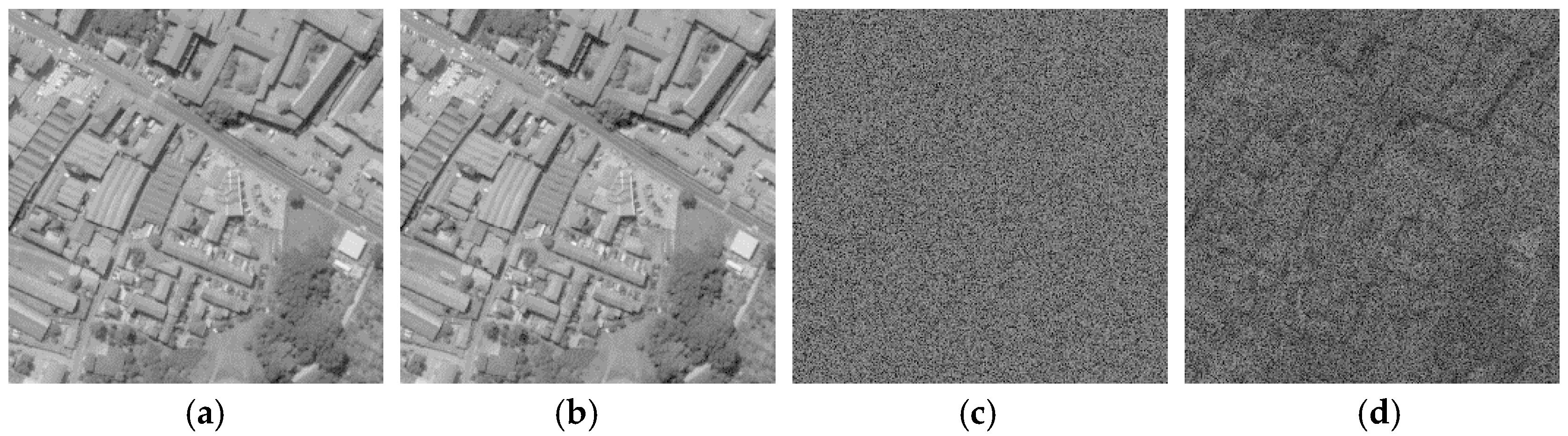
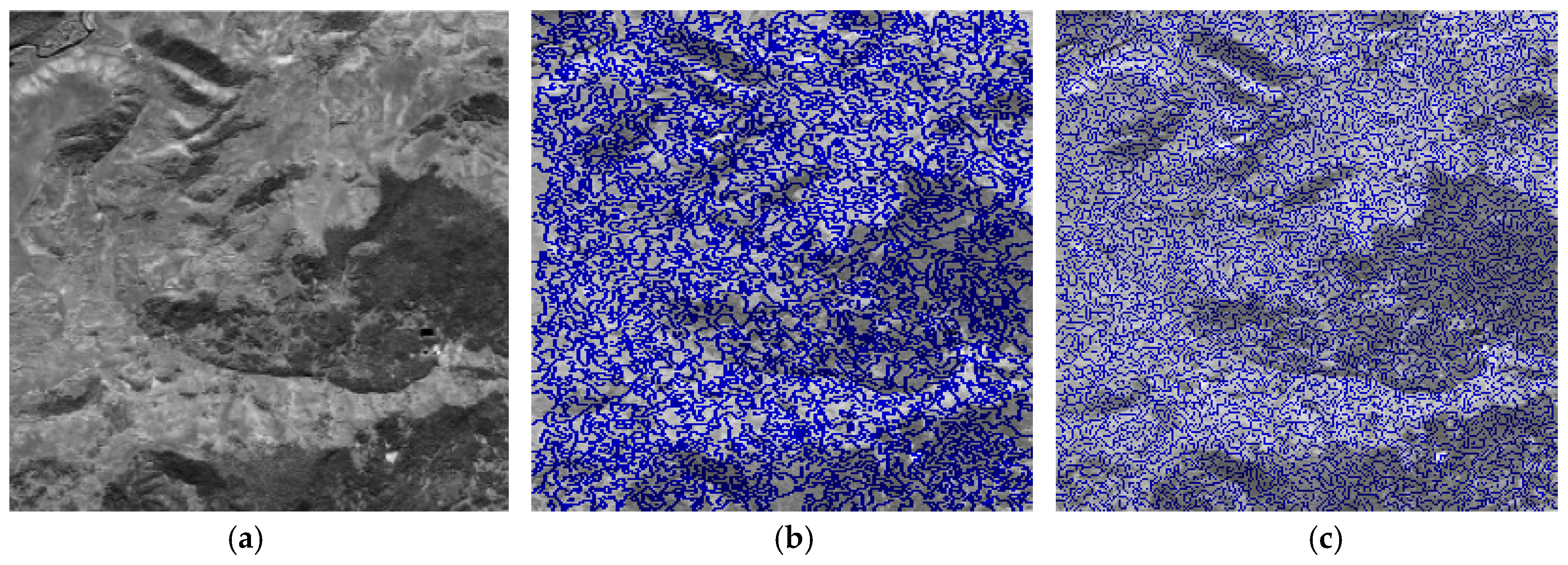
In this experiment, 30 dB noise is added to each band of HSI. According to the definition of SNR, the noise power in each band is proportional to the power of the noise-free signals in the corresponding band. Since the intensity varies with the wavelength, the noise level varies with the wavelength. The ratio of the SI noise power to the SD noise power is 1:1, that is to say, the power of SI noise and SD noise is competitive, none of which can be ignored when estimated. In Figure 1a,b, it is difficult for human eyes to distinguish the slight difference between the noise-free data and the noisy data of 30 dB noise. However, in many HSI post-processing methods that are sensitive to noise, 30 dB is high enough to reduce the performance significantly [28,29]. Therefore, we first choose 30 dB noise with $\alpha =1:1$ for the experiment.

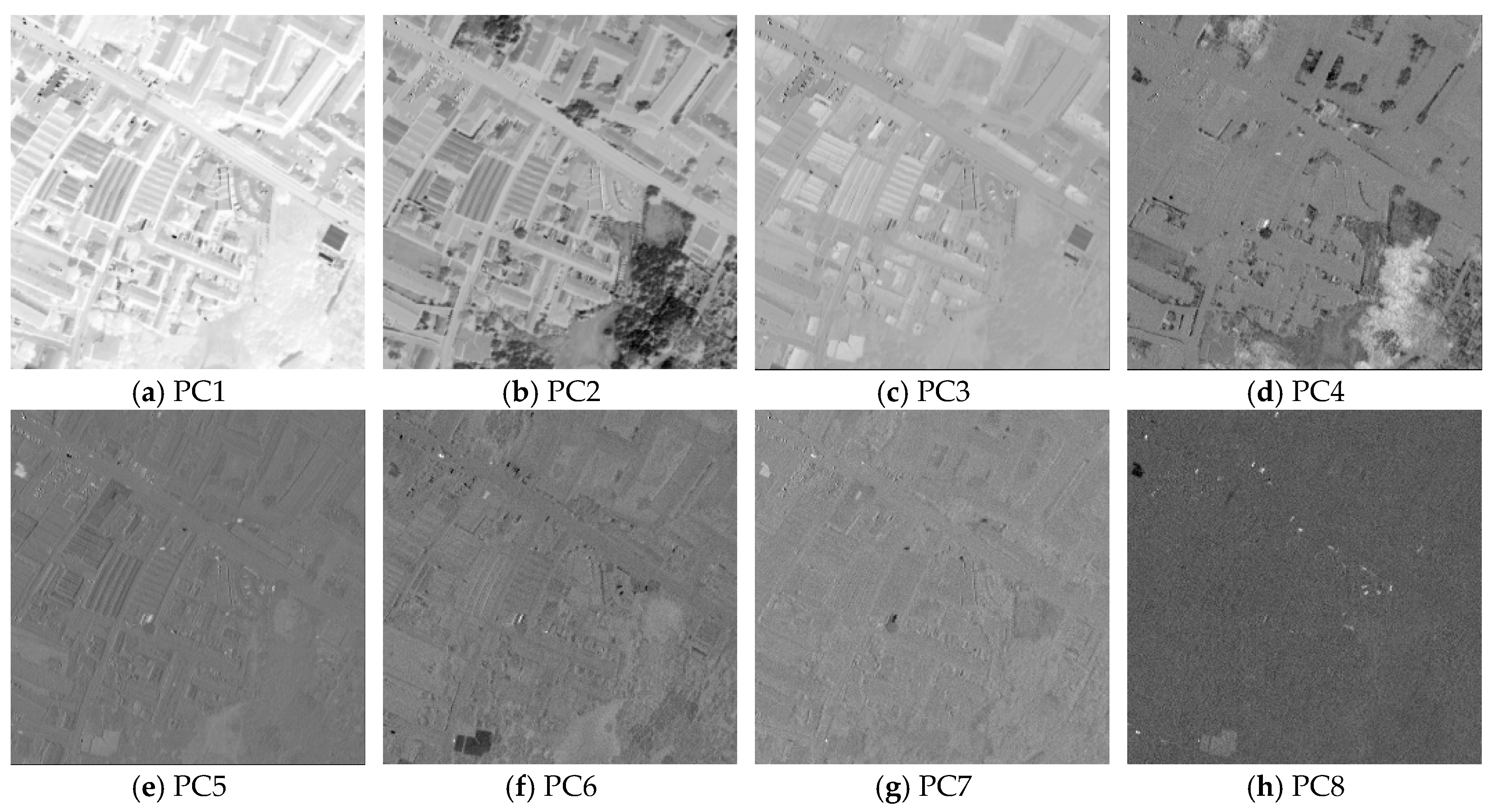
The first step of the algorithm is MNF. Figure 2 gives the top eight PCs obtained by MNF with the dataset Pavia Centre. The first PC has the strongest signal power, while the following PCs contain less signal power. Since the noise in HSI has been processed by the noise-whitening matrix, the first PC has the highest SNR compared to the other PCs. This advantage ensures the performance of the subsequent superpixel segmentation.

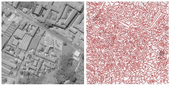
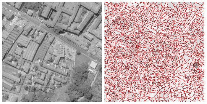
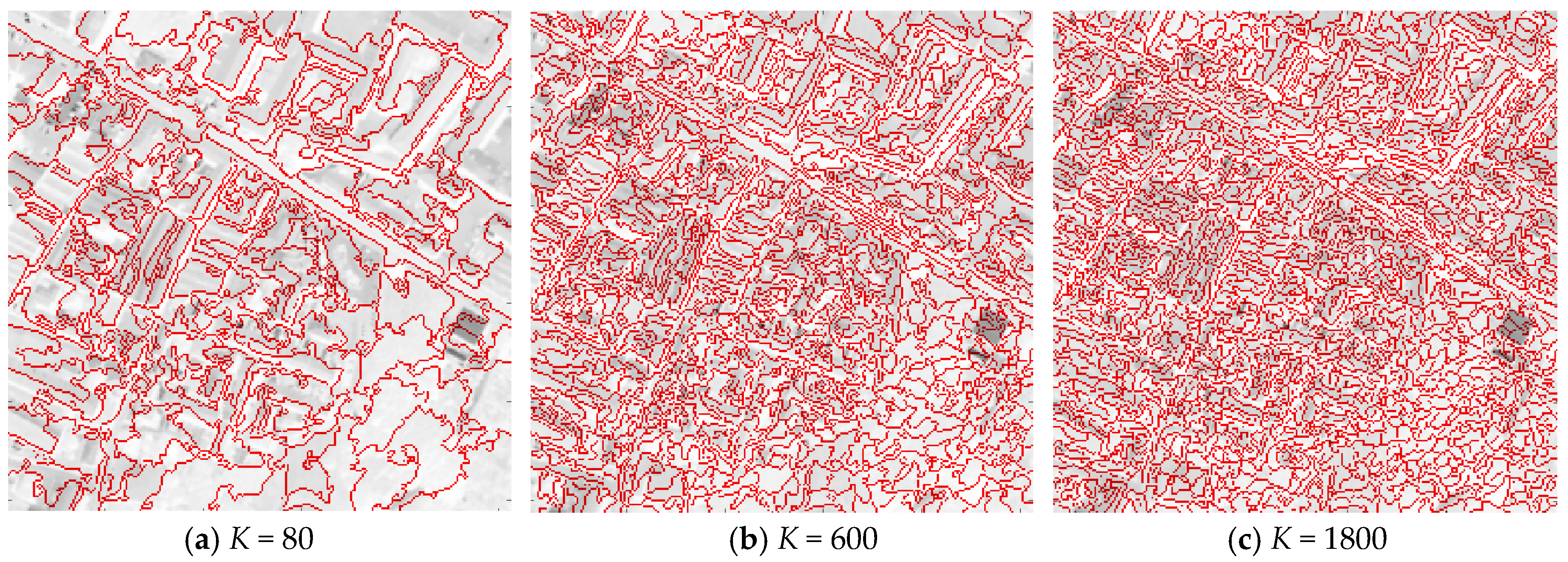
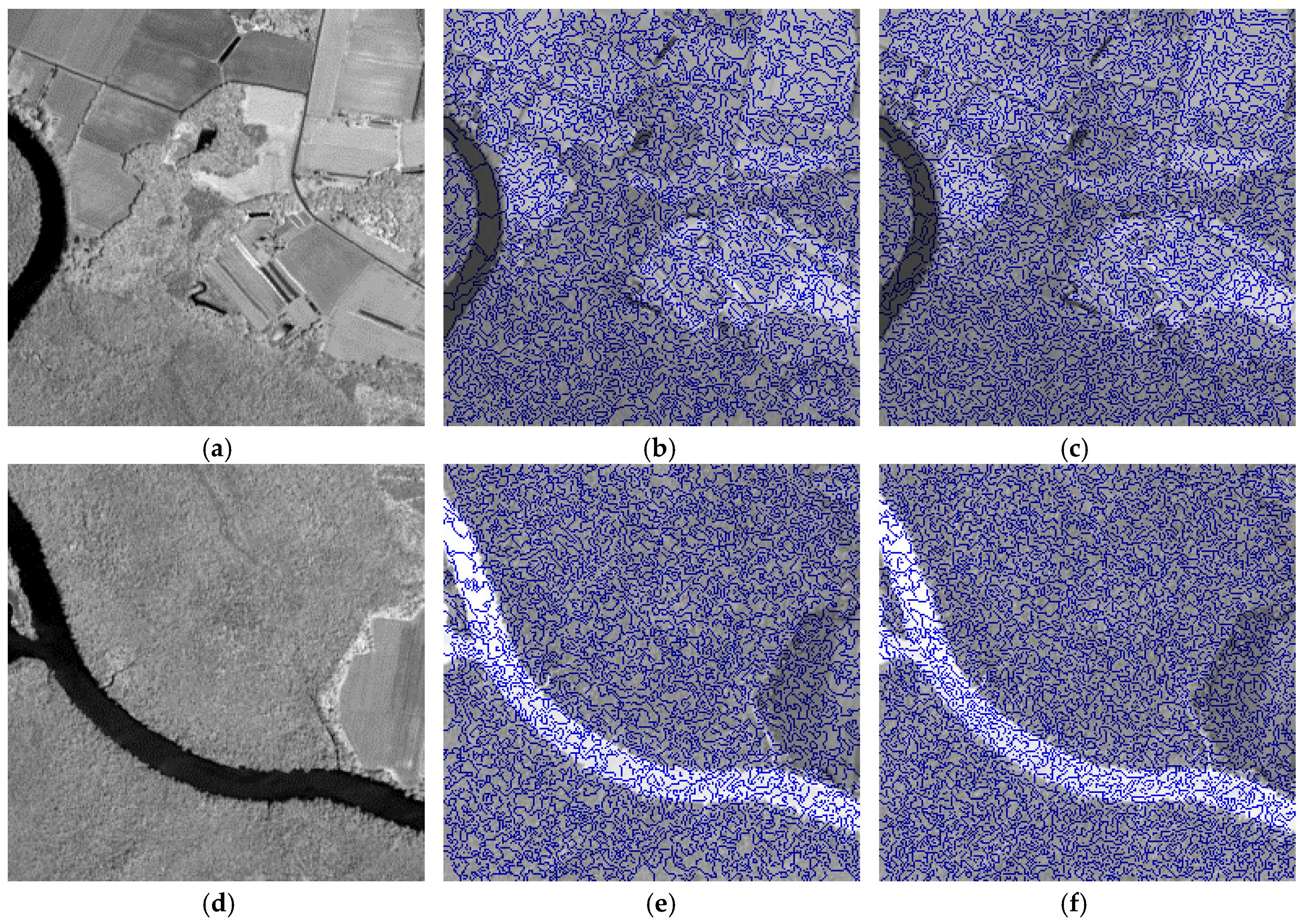
The superpixel segmentation results achieved by the ERS on PC1 are given in Figure 3, where the superpixel number K is 80, 600 and 1200. Note that the superpixel number has a direct impact on the final noise estimation result. Therefore, it is necessary to determine a reasonable number K.

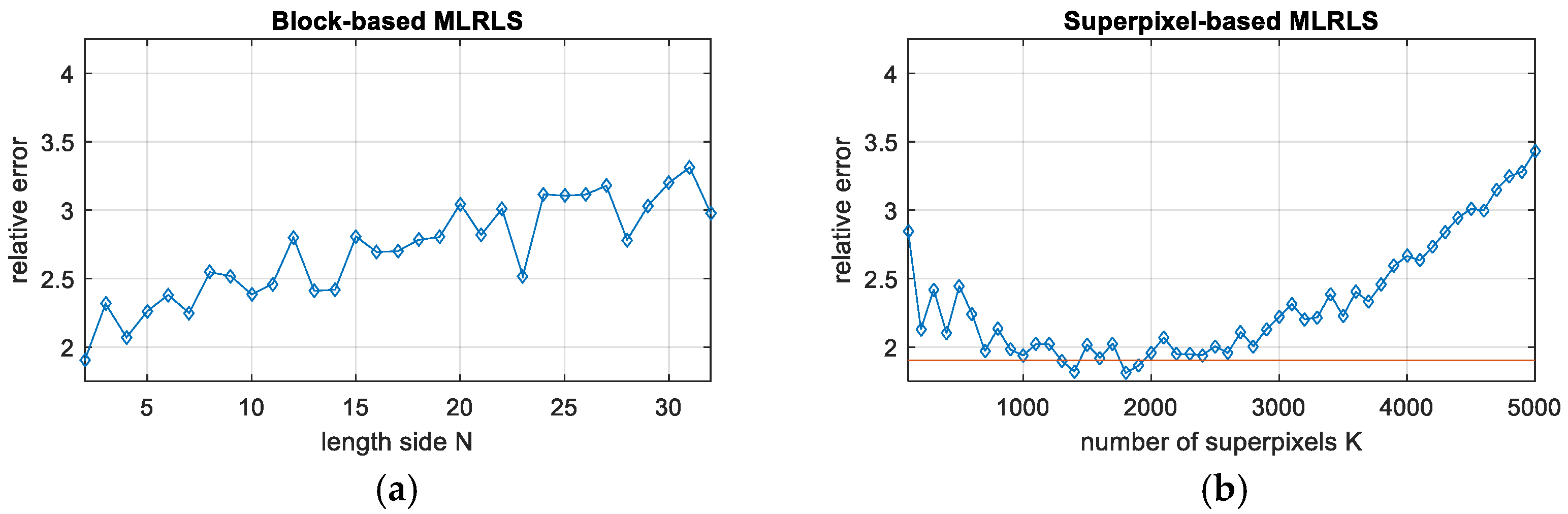
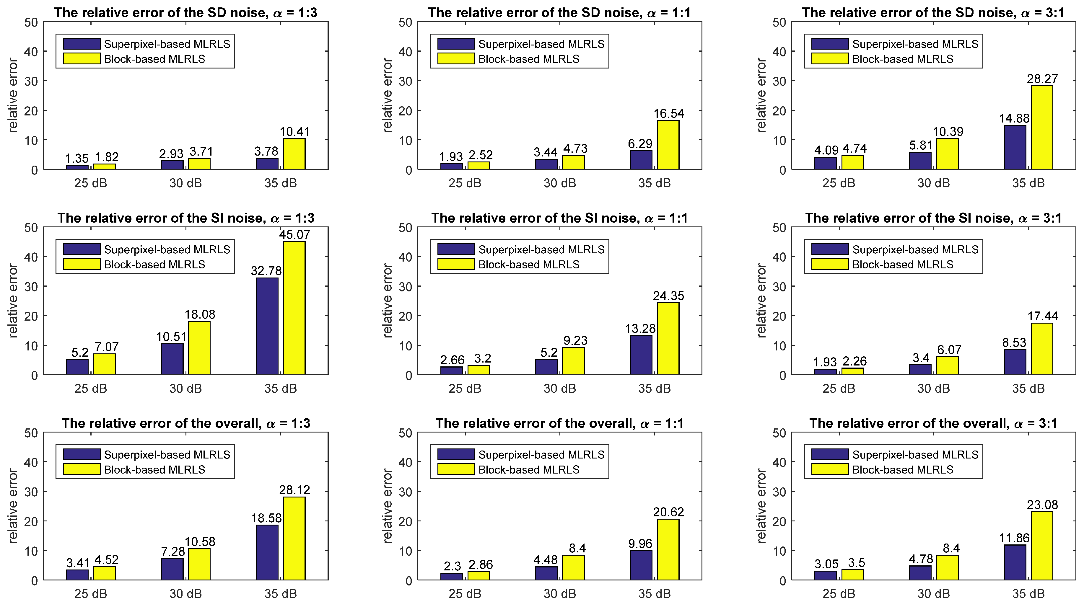
In the block-based MLRLS [21], the size of a block is 7 × 7. In this paper, more sizes N × N (height $\times$ width) each of them is viewed, where N ranges from 2 to 32. Meanwhile, in order to find a proper number K of the superpixels in the superpixel-based MLRLS, different numbers K are tested from 100 to 5000 with a step size of 100. The relative errors of the SD noise estimated by the block-based MLRLS and the superpixel-based MLRLS are given in Figure 4. The minimal relative error of the block-based MLRLS is 1.90%, with the length side of a block being $N=2$. When N is in a range from 2 to 7, the relative error varies stably in a narrow interval (1.90, 2.38). The blue curve in Figure 5b shows the relative error of the SD noise estimated by the superpixel-based MLRLS, and the red line is the minimal relative error of the block-based MLRLS. When $K$ is in a wide interval [900, 2600], the relative error fluctuates slightly along the red line, and is limited in a narrow interval (1.81, 2.07). The minimal relative error for the superpixel-based MLRLS is 1.81%, with $K=1800$.

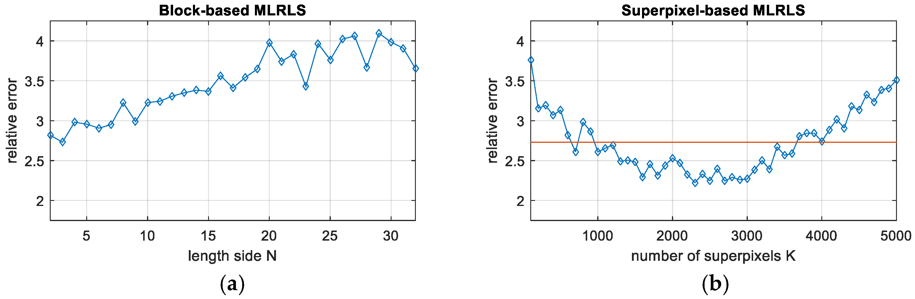
Figure 5 shows the relative errors of the SI noise estimated by the block-based MLRLS and the superpixel-based MLRLS. In Figure 5a, the minimal relative error of the block-based MLRLS is 2.73%, with $N=3$. When N is in the range from 2 to 7, the relative error varies stably and is limited in a narrow interval (2.73, 2.98). Figure 5b shows the relative errors of the SI noise estimated by the superpixel-based MLRLS. The minimal relative error of the superpixel-based MLRLS is 2.22%, with $K=2300$. When $K$ is in a wide interval [1000, 3600], all the values of the relative errors are below the red line. This means that the number of superpixels $K$ taken in a large range can ensure that the relative error is smaller than that of the block-based MLRLS. Meanwhile, when $K$ is in the interval (1300, 3300), the relative error fluctuates slightly in a narrow interval (2.22, 2.53).

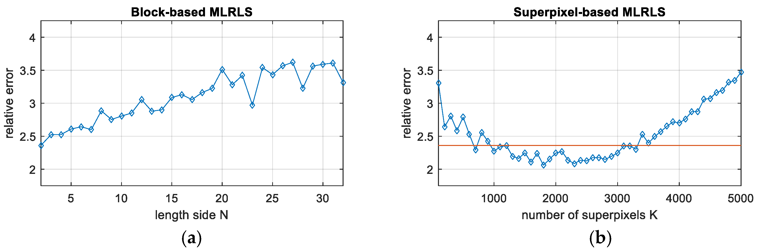
Since the relative errors of both the SD noise and the SI noise do not always achieve the minimal value at the same point N or $K$, the average value of the relative errors of the SD noise and the SI noise is also tested for an overall optimization. Figure 6 shows the relative errors for the overall optimization taking both the SD and SI noise into account. The minimal relative error of the block-based MLRLS is 2.36%, with $N=2$. When N is in a range of 2 to 7, the relative error varies stably in a narrow interval (2.36, 2.64). As N becomse large, the general trend of the relative error becomes large. The reason for this phenomenon is that when the size of a block becomes large, it will contain more types of ground objects in an identical block, which will lead to inhomogeneous regions in one block and violate to assumption of homogeneity. In Figure 6b, the minimal relative error of the superpixel-based MLRLS is 2.06%, with $K=1800$. When $K$ is in a wide interval [1000, 3300], all the relative errors of the superpixel-based MLRLS are smaller than the minimal relative error of the block-based MLRLS. Meanwhile, when $K$ is in the range of (1300, 3300), the relative error fluctuates slightly in a narrow interval (2.06, 2.27).

By the comparison, the minimal relative error of the noise with $K=1800$ estimated by the superpixel-based MLRLS is smaller than that of the block-based MLRLS with $N=2$. However, the selection of the optimal length side of a block $N$ in the block-based MLRLS and the optimal number of superpixels $K$ in the superpixel-based MLRLS is dependent of the HSI dataset, and involves many factors such as the noise level, the edges, etc. The above experimental analysis indicates that the superpixel-based MLRLS can still perform better than the block-based MLRLS with a wide selection of $K$ when the ground truth noise is unknown.

5.1.2. Experiments for Different Cases

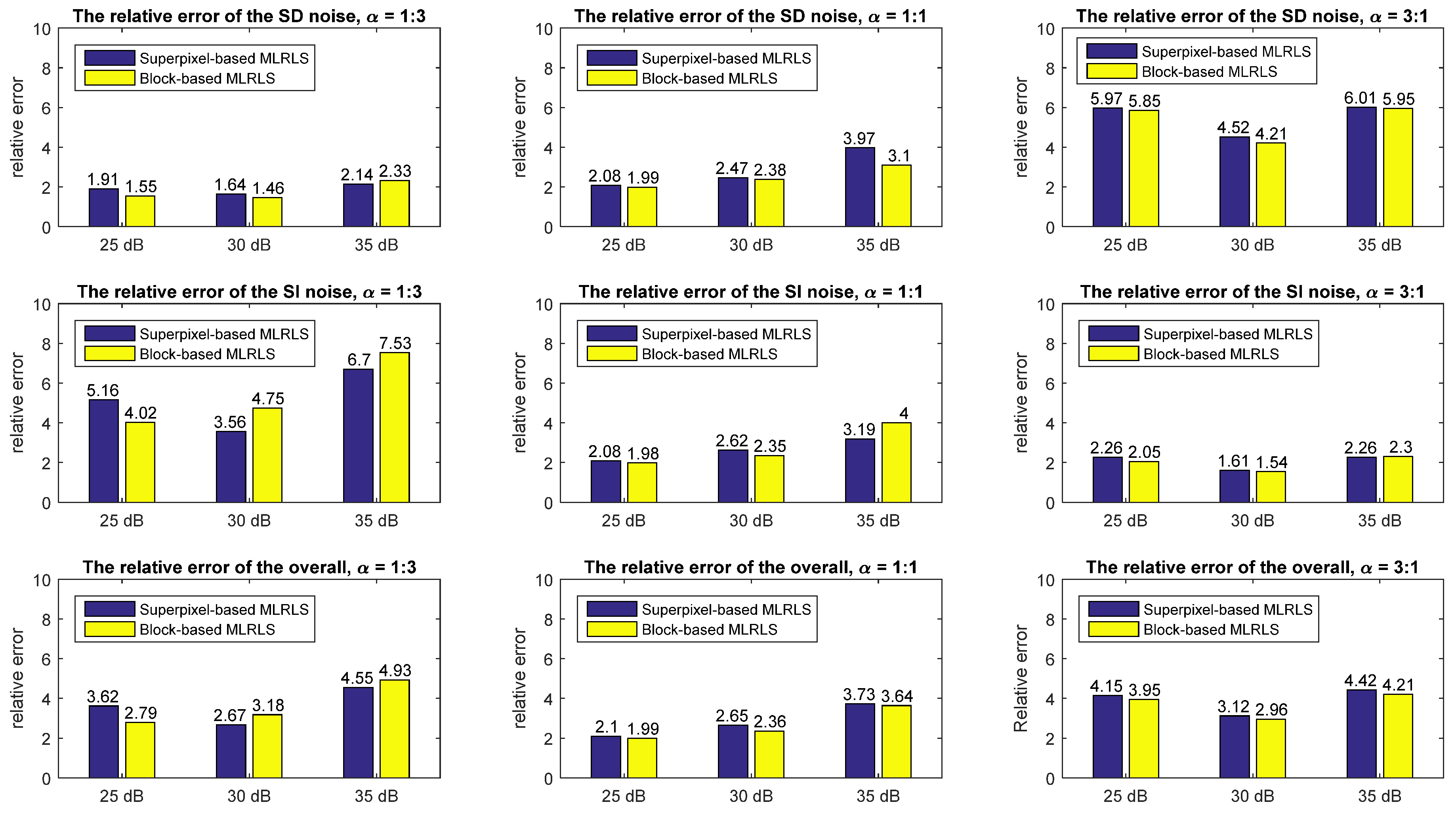
In this section, the algorithm is carried out on HSIs with different noise levels and different noise components. 25 dB, 30 dB and 35 dB noises with different $\alpha$ are added on the hyperspectral dataset Pavia Centre.

Table 1. The optimal relative errors of the SD noise, the SI noise and the overall optimization.

SNR	$\mathit{\alpha }$	Superpixel-Based MLRLS			Block-Based MLRLS [21]			MLRML [19]
		SD	SI	Overall	SD	SI	Overall	SD	SI	Overall
25 dB	1:3	1.38	3.61	2.60	1.39	4.04	2.73	5.37	10.56	7.97
	1:1	1.79	1.79	1.81	1.59	1.87	1.73	6.15	7.14	6.64
	3:1	2.87	1.16	2.02	3.00	1.18	2.09	9.37	5.78	7.58
30 dB	1:3	1.55	4.62	3.36	1.68	5.81	3.76	8.65	20.59	14.62
	1:1	1.81	2.22	2.06	1.90	2.73	2.36	10.53	13.03	11.78
	3:1	3.85	1.60	2.82	4.34	1.88	3.15	11.78	10.31	13.23
35 dB	1:3	1.84	8.94	5.72	2.85	11.8	7.46	15.80	37.47	26.63
	1:1	2.84	4.35	3.69	4.44	6.47	5.62	18.72	26.75	22.74
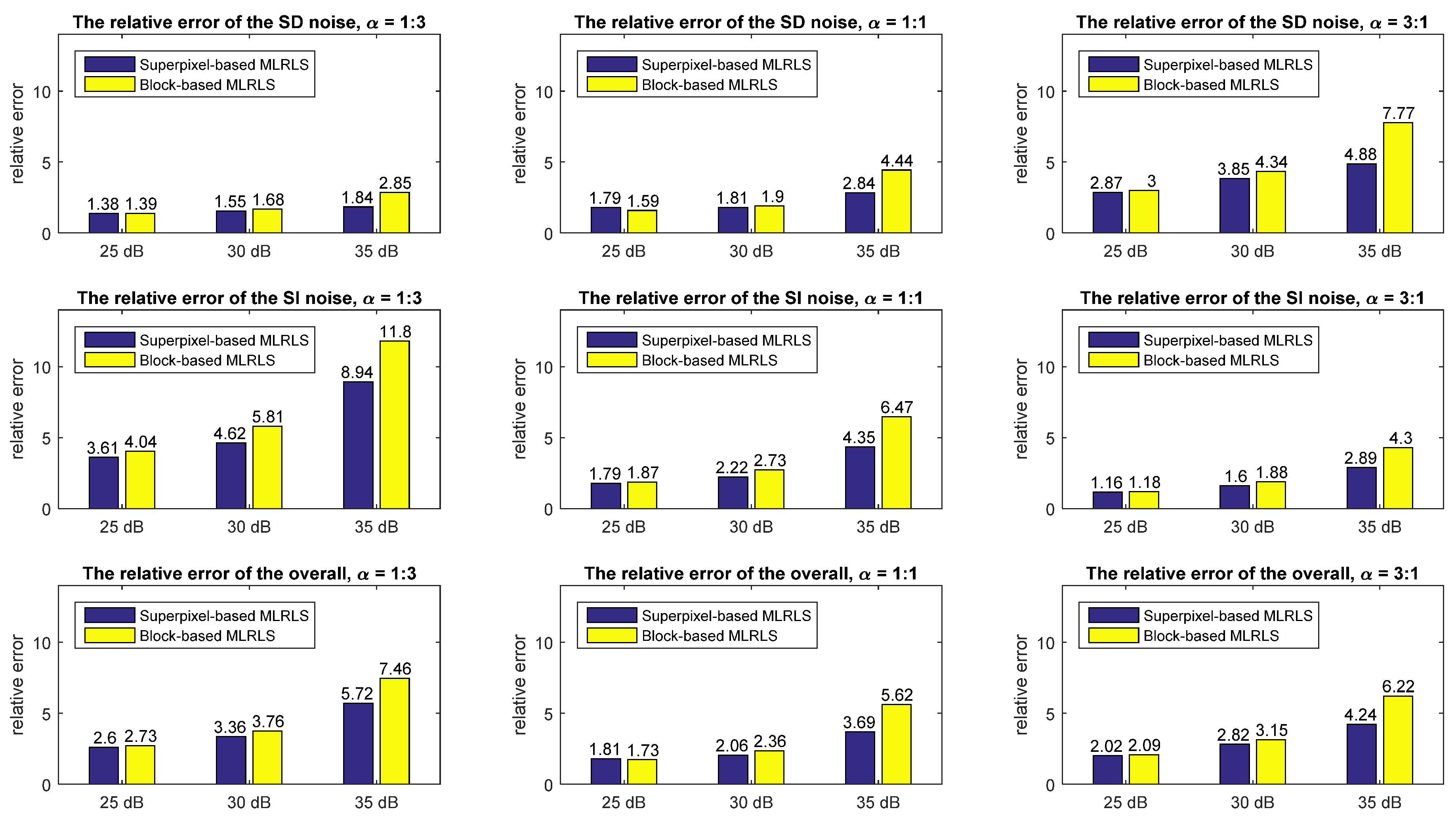
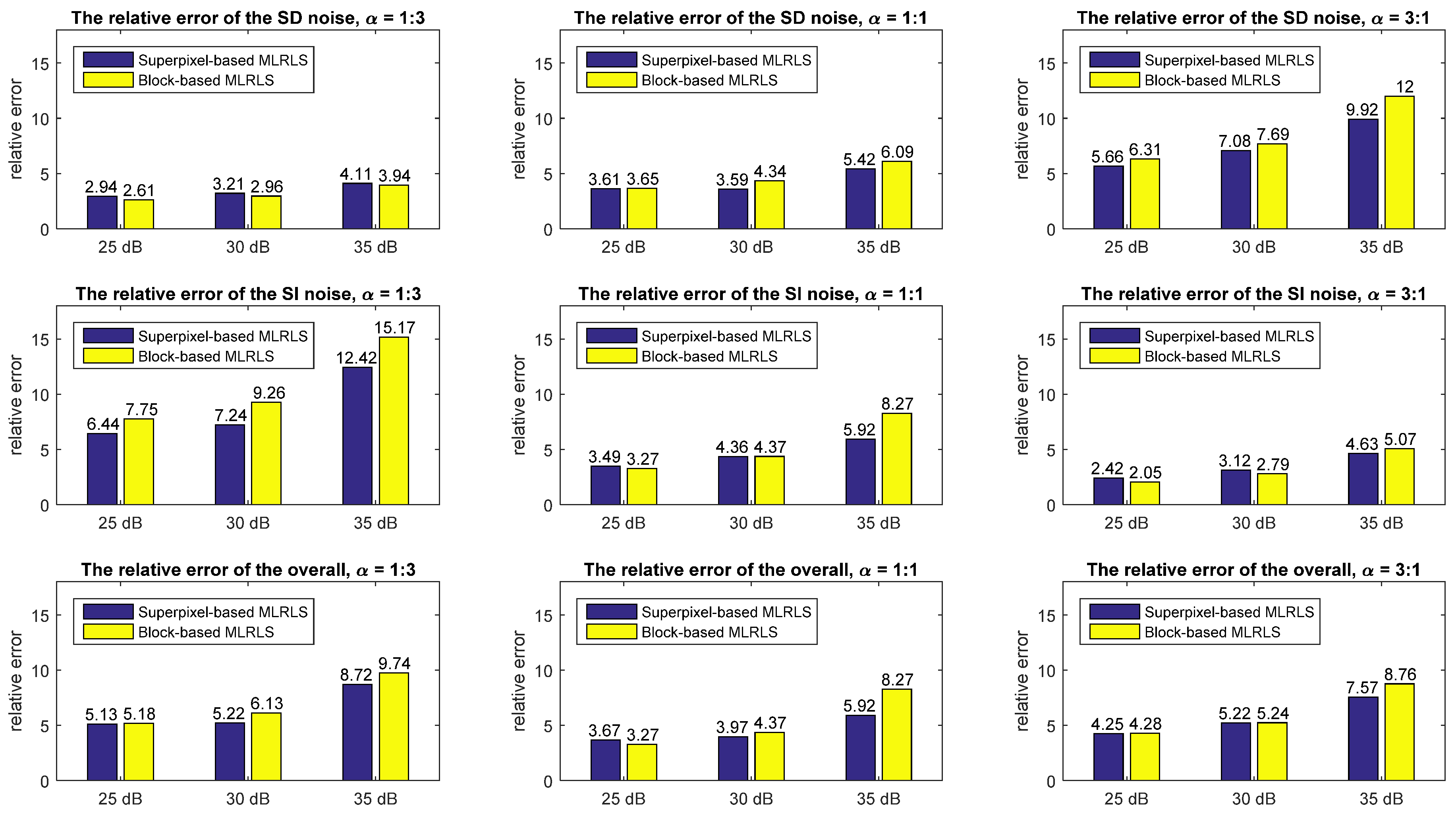
	3:1	4.88	2.89	4.24	7.77	4.30	6.22	28.33	19.40	23.87

and Figure 7 show the relative errors of the superpixel-based MLRLS, the block-based MLRLS [21], and MLRML [19].

When SNR = 25 dB, the proposed algorithm does not improve much in terms of the relative errors. When $\alpha =1:3$, the overall relative error is only reduced by 0.13%, and when $\alpha =3:1$, the overall relative error is only reduced by 0.07%. When $\alpha =1:1$, the accuracy is slightly decreased. At low SNR, the high level noise affects the accuracy of superpixel segmentation and subsequently degrades the performance of the proposed algorithm. Therefore, when the noise level is high, the superiority of the superpixel-based MLRLS is not obvious over the block-based MLRLS. When SNR = 30 dB, the overall relative error of the superpixel-based MLRLS is 0.34% less than that of the block-based MLRLS, while when SNR = 35 dB, the overall relative error is 1.88% less than that of the block-based MLRLS, and the estimation accuracy is improved by 1.01%–2.89%. As the SNR becomes larger, the superpixel segmentation performs better. 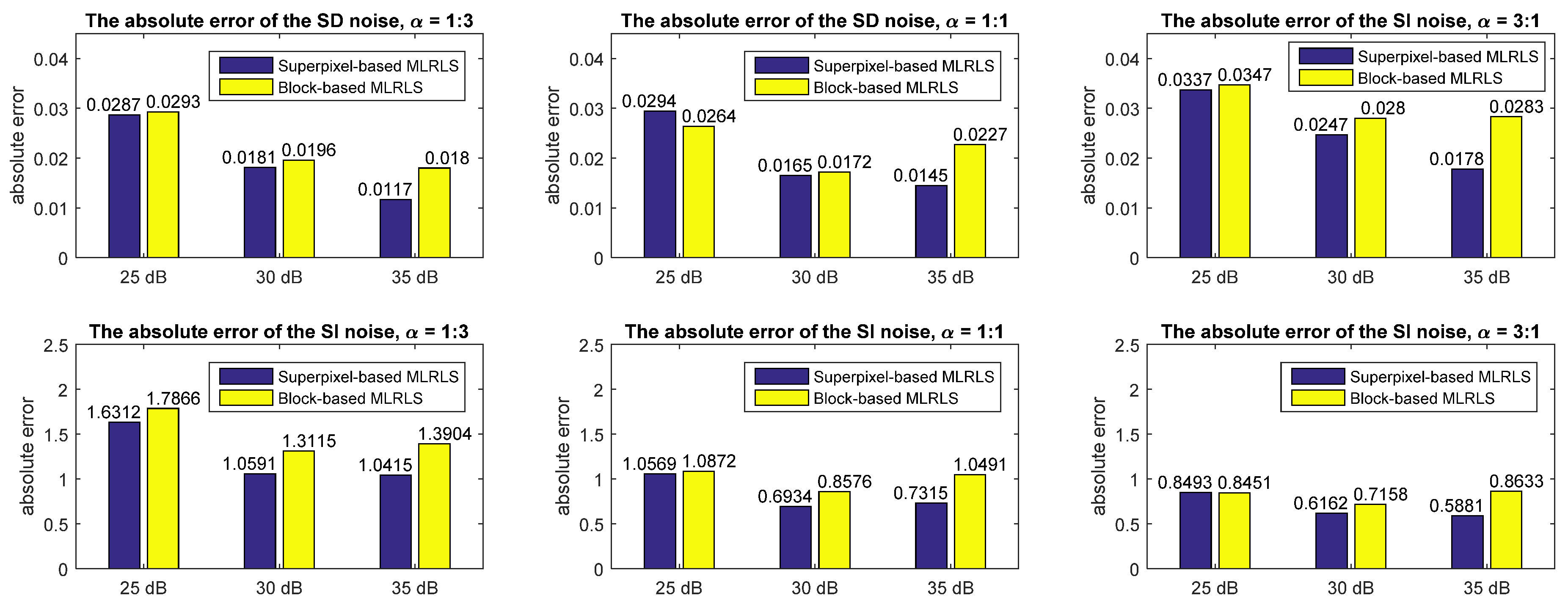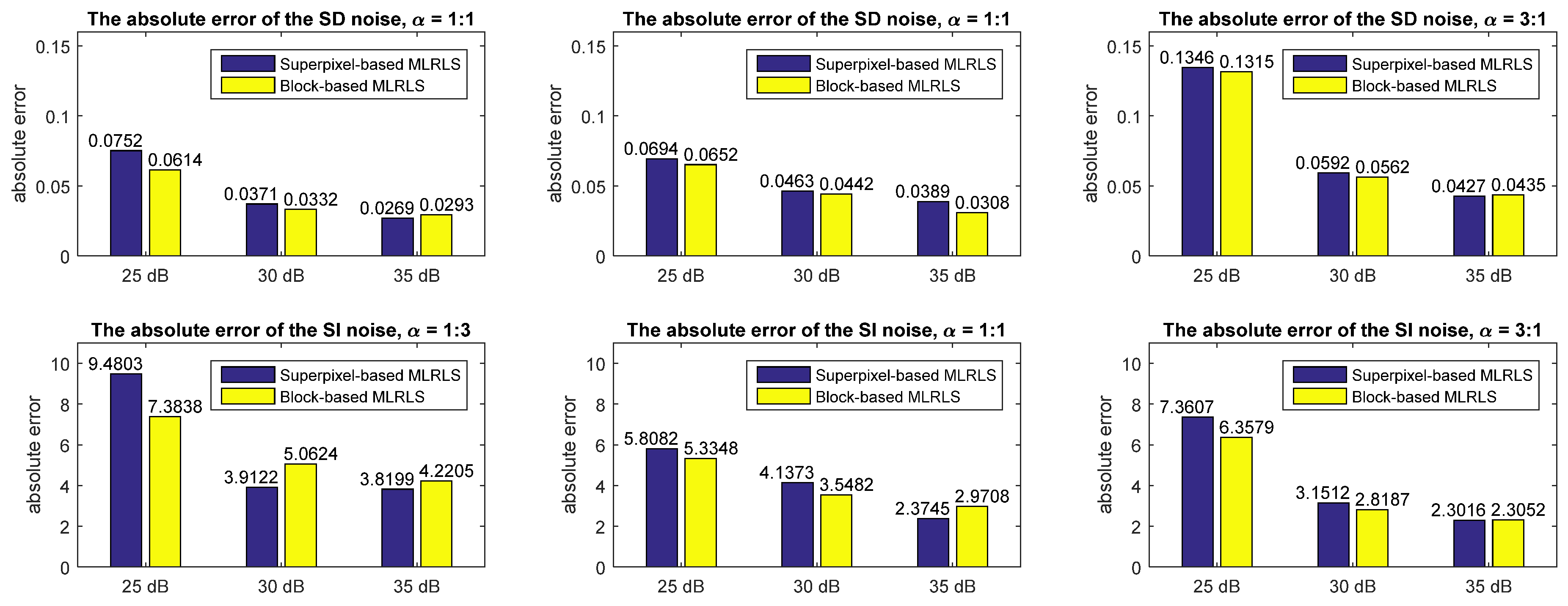Therefore, Table 1 shows that the superpixel-based MLRLS outperforms the block-based MLRLS, especially for high-SNR images. In addition, the absolute errors are listed in

Table 2. The optimal absolute errors of the SD noise, the SI noise and the overall optimization.

SNR	$\mathit{\alpha }$	Superpixel-Based MLRLS		Block-Based MLRLS [21]		MLRML [19]
		SD	SI	SD	SI	SD	SI
25 dB	1:3	0.0287	1.6312	0.0293	1.7866	0.1089	4.1249
	1:1	0.0294	1.0569	0.0264	1.0872	0.1008	4.1132
	3:1	0.0337	0.8493	0.0347	0.8451	0.1098	4.0398
30 dB	1:3	0.0181	1.0591	0.0196	1.3115	0.0979	4.5613
	1:1	0.0165	0.6934	0.0172	0.8576	0.0976	4.1007
	3:1	0.0247	0.6162	0.0280	0.7158	0.1058	4.0144
35 dB	1:3	0.0117	1.0415	0.0180	1.3904	0.1003	4.7284
	1:1	0.0145	0.7315	0.0227	1.0491	0.0974	4.7169
	3:1	0.0178	0.5881	0.0283	0.8633	0.1047	4.2560

and Figure 8. These figures indicate that the absolute errors decrease with a higher SNR. Meanwhile, the MNF approach and using superpixel segmentation to find homogenous regions play an important role in the mixed noise estimation, especially for HSIs of high SNRs.

A bar plot of Table 1 is given in Figure 7. As shown in Table 1 and Figure 7, the relative error becomes large as the SNR increases. However, this does not mean that a high SNR may lead to poor performance. In fact, a high SNR can ensure the performance of superpixel segmentation, which improves accuracy in terms of the absolute error. Since the standard deviations of the SD noise and the SI noise vary greatly in magnitude, to compare them at the same level, the relative error ${\epsilon }_r=\left|\widehat{\sigma }-\sigma \right|/\sigma \times 100\%$ is introduced for normalization. In ${\epsilon }_r=\left|\widehat{\sigma }-\sigma \right|/\sigma \times 100\%$, if $\sigma$ becomes smaller, ${\epsilon }_r$ becomes larger. That is to say, $\sigma$ is smaller with a higher SNR, accordingly, the relative error ${\epsilon }_r$ becomes larger. To eliminate this misunderstanding that a high SNR leads to poor performance, the absolute errors $\left|\widehat{\sigma }-\sigma \right|$ are also calculated in the experiments. Table 2 and Figure 8 show the absolute errors at different noise levels and in different cases. When the SNR is higher, the absolute errors are smaller. 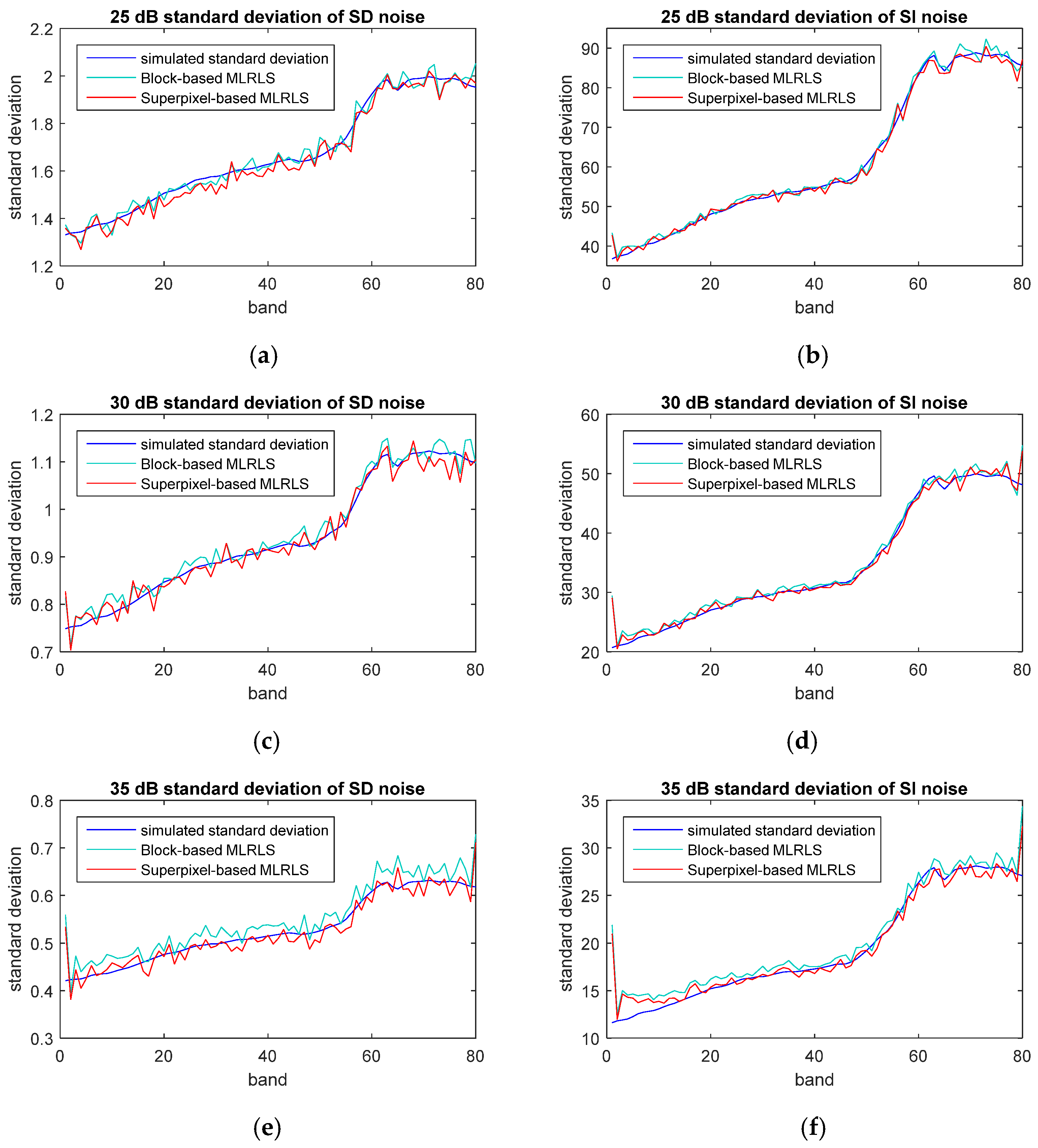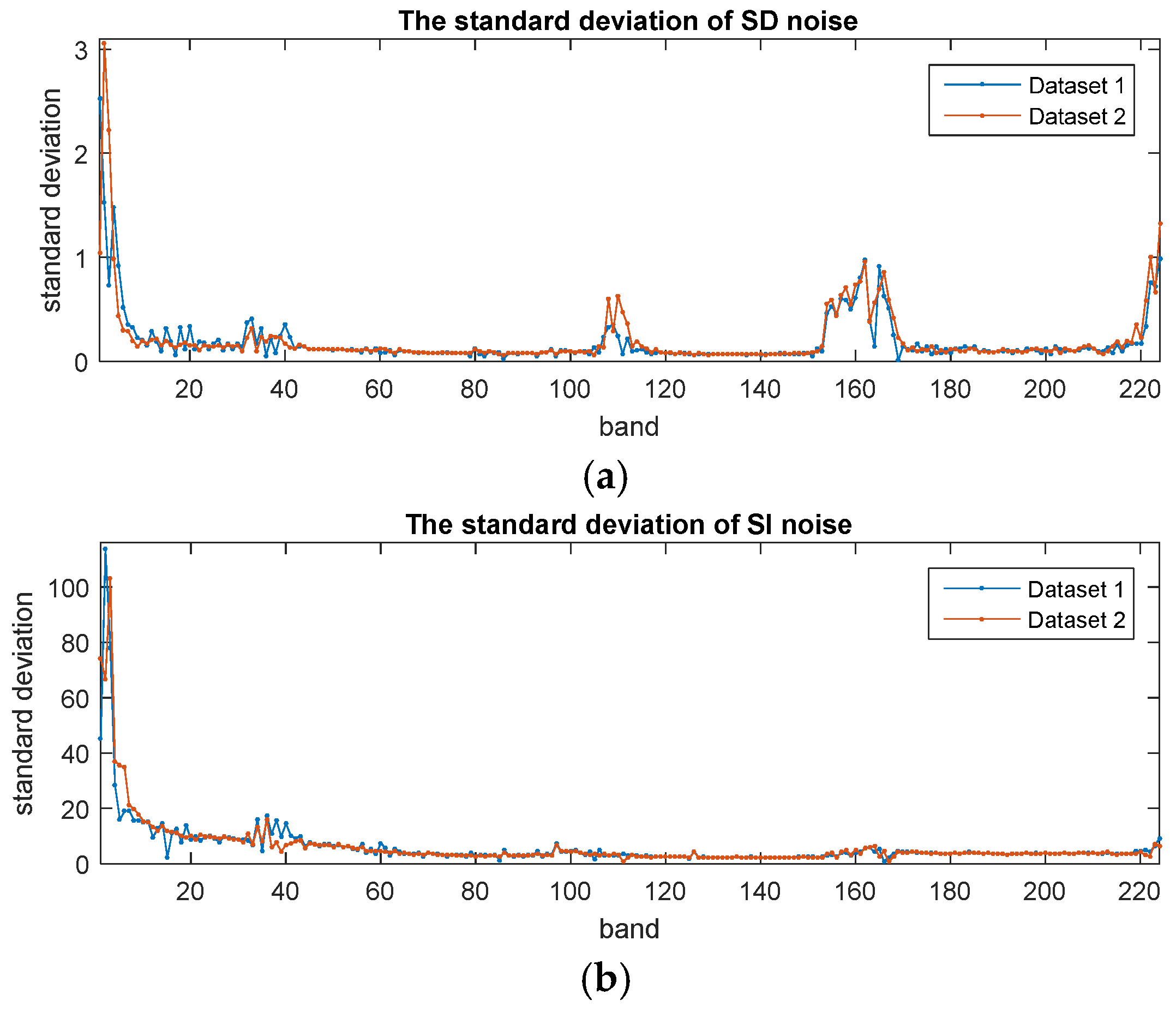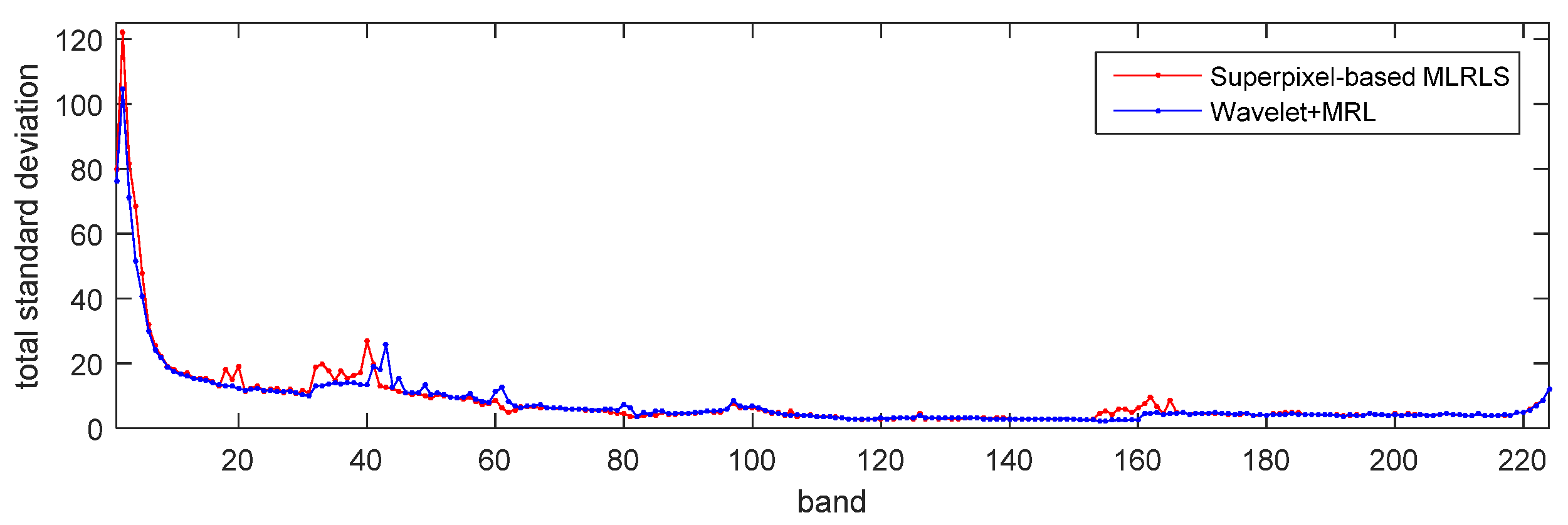Figure 9 shows the standard deviation of the estimated SD and SI noise in each band compared with that of the synthetic noise, when $\alpha =1:1$, and SNR = 25 dB, 30 dB and 35 dB, respectively. When SNR = 35 dB, the curve of the standard deviation of the superpixel-based MLRLS is obviously closer to that of the synthetic noise than that of the block-based MLRLS.

Furthermore, the proposed algorithm is compared with the MLRML method [19]. The MLRML only takes high spectral correlation into account, but ignores spatial correlation. When SNR = 25 dB, the noise level is high, the performance of the noise estimation achieved by the MLRML is acceptable. When the noise level is low, the MLRML fails to distinguish subtle difference between the noise and the details of the HSIs, which leads to an inaccurate noise estimation.

The experimental results with different noise levels and different noise components indicate that with the development of imaging quality using modern spectrometers, the proposed algorithm the superpixel-based MLRLS is more suitable for the noise estimation of modern HSI datasets.

Next, we will discuss the selection of the side length $N$ of a block in the block-based MLRLS and the number of the superpixels $K$ in the superpixel-based MLRLS at different noise levels.

Table 3. The side length N of the optimal relative errors for the block-based MLRLS.

SNR	$\mathit{\alpha }$	The Side Length N of a Block
		SD	SI	Overall
25 dB	1:3	8	5	5
	1:1	6	6	6
	3:1	2	2	2
30 dB	1:3	4	5	5
	1:1	2	3	2
	3:1	5	6	5
35 dB	1:3	2	3	3
	1:1	2	5	5
	3:1	2	6	2

shows the side length $N$ when the block-based MLRLS gets the optimal relative errors at different noise levels. It indicates that $N$ fluctuates in a range from 2 to 8, and the average value of $N$ is 4.04. Therefore, $N=4$ is recommended for the block-based MLRLS performed on the real-life data when the ground truth noise is unknown.

Table 4. The number of superpixels K of the optimal relative error for the superpixel-based MLRLS.

SNR	$\mathit{\alpha }$	The Number of Superpixels K
		SD	SI	Overall
25 dB	1:3	800	2400	800
	1:1	800	1400	1400
	3:1	1100	800	800
30 dB	1:3	1400	3200	1800
	1:1	1800	2300	1800
	3:1	2400	1000	2200
35 dB	1:3	3000	5200	4700
	1:1	4200	5100	5000
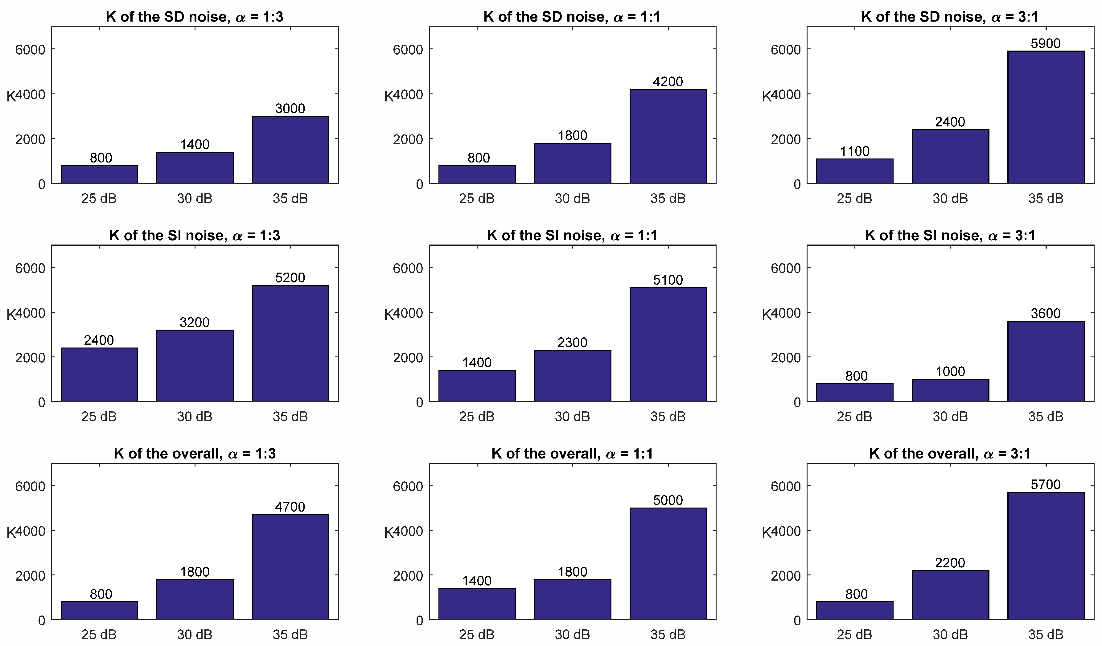
	3:1	5900	3600	5700

and Figure 10 show the number of superpixels $K$ when the superpixel-based MLRLS achieves the optimal relative errors at different noise levels. As can be seen, the optimal $K$ is from 800 to 5700, and the average value of $K$ is 2614.8, i.e., on average, 25 pixels in a superpixel. Meanwhile, when SNR = 25 dB, the average value of $K$ is 1144.4, i.e., on average, 57 pixels in one superpixel; when SNR = 30 dB, the average value of $K$ is 1988.9, i.e., on average, 33 pixels in one superpixel; when SNR = 35 dB, the average value of $K$ is 4711.1, i.e., on average, 14 pixels in one superpixel. Thus, the selection of $K$ is dependent on the noise level of the HSIs. Therefore, it is recommended that on average, 25 pixels in one superpixel is selected in the superpixel-based MLRLS. If the noise level is high, one can choose more pixels in a superpixel, i.e., a smaller $K$, and vice versa.

Table 5. The computational time of the superpixel-based MLRLS and the block-based MLRLS (unit: second).

SNR	$\mathit{\alpha }$	Superpixel-Based MLRLS			Block-Based MLRLS [21]
		SD	SI	Overall	SD	SI	Overall
25 dB	1:3	10.02	20.25	9.83	9.47	20.05	19.78
	1:1	9.93	13.89	13.59	14.36	14.16	13.89
	3:1	11.78	9.48	9.66	127.33	130.08	128.17
30 dB	1:3	13.80	24.77	16.17	29.81	20.19	19.69
	1:1	16.41	18.86	16.42	128.38	50.02	127.31
	3:1	20.66	11.00	18.84	19.63	14.08	19.84
35 dB	1:3	24.08	37.47	33.63	133.97	50.60	49.42
	1:1	30.69	36.34	34.14	132.13	19.58	19.88
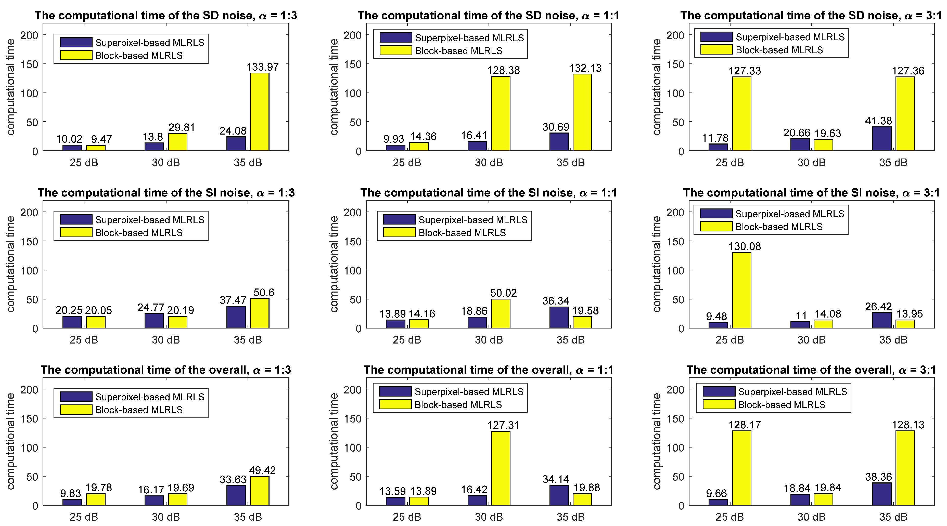
	3:1	41.38	26.42	38.36	127.36	13.95	128.13

and Figure 11 show the computational time of the two algorithms. The algorithms are compiled and run in Matlab R2015a. The computer processor is Intel(R) Core(TM) i7-10710U CPU @1.10GHz and 1.61GHz, and the memory capacity is 16.0 GB. The average computational time of the superpixel-based MLRLS is 21.03 s, while the average computational time of the block-based MLRLS is 58.57 s. In the superpixel-based MLRLS, the computational time of MNF is 1.33 s, on average. The superpixel segmentation used in the proposed algorithm is based on a greedy optimization scheme, and is only performed on the first component. Therefore, the computational cost is not expensive. The superpixel segmentation takes only 0.32 s, on average. Most of the computational time is spent on calculating the matrix elements in Equations (24)–(26) and the least-squares method in Equation (28). The computational complexity is dependent on the number of superpixels or the number of blocks. Since the average number of superpixels K is 2614.8, while the average side length N of a block is 4.04, i.e., 16,222 blocks in the tested HSI data, the average computational time of the superpixel-based MLRLS is much lower than the block-based MLRLS.

5.1.3. Experiments on Low-Resolution Datasets

The proposed algorithm is based on the assumption that the HSIs have large spatial and spectral resolution. In this section, we discuss how lower spatial and spectral resolution affect the estimation performance of the proposed algorithm.

A. Lower Spatial Resolution

In this experiment, spatial subsampling is performed on the HSI dataset Pavia Centre to obtain a lower spatial resolution. The dataset is subsampled by 1:2 in spatial rows and 1:2 in columns, respectively. Thus, the subsampled dataset has a spatial resolution of 1:4 of the original image. The superpixel-based MLRLS and the block-based MLRLS are performed on the subsampled dataset. The estimated relative error is shown in

Table 6. The optimal relative errors of the SD noise, the SI noise and the overall optimization for 1:4 spatial subsampling HSI.

SNR	$\mathit{\alpha }$	Superpixel-Based MLRLS			Block-Based MLRLS [21]
		SD	SI	Overall	SD	SI	Overall
25 dB	1:3	2.94	6.44	5.13	2.61	7.75	5.18
	1:1	3.61	3.49	3.67	3.65	3.27	3.46
	3:1	5.66	2.42	4.25	6.31	2.05	4.28
30 dB	1:3	3.21	7.24	5.22	2.96	9.26	6.13
	1:1	3.59	4.36	3.97	4.34	4.37	4.35
	3:1	7.08	3.12	5.22	7.69	2.79	5.24
35 dB	1:3	4.11	12.42	8.72	3.94	15.17	9.74
	1:1	5.42	5.92	5.92	6.09	8.27	7.29
	3:1	9.92	4.63	7.57	12.00	5.07	8.76

and Figure 12. This indicates that after spatial subsampling, the estimation errors of the two algorithms decrease compared to higher spatial resolution images. The estimated relative error of the superpixel-based MLRLS decreases by 1.26%–5.04%, with an average decrease of 2.33%. The estimated relative error of the block-based MLRLS decreases by 0.77%–4.23%, with an average decrease of 2.14%.

Although the lower spatial resolution makes the estimation accuracy of the superpixel-based MLRLS decreased slightly more than that of the block-based MLRLS, the estimation accuracy of the superpixel-based MLRLS in most cases is still higher than that of the block-based MLRLS.

B. Lower Spectral Resolution

Spectral subsampling is also performed on the HSI Pavia Centre to obtain a lower spectral resolution. The dataset is subsampled by 1:2 in the spectrum. The superpixel-based MLRLS and the block-based MLRLS are performed on the subsampled dataset. The estimated relative error is shown in

Table 7. The optimal relative errors of the SD noise, the SI noise and the overall optimization for 1:2 spectral subsampling HSI.

SNR	$\mathit{\alpha }$	Superpixel-Based MLRLS			Block-Based MLRLS [21]
		SD	SI	Overall	SD	SI	Overall
25 dB	1:3	1.35	5.20	3.41	1.82	7.07	4.52
	1:1	1.93	2.66	2.30	2.52	3.20	2.86
	3:1	4.09	1.93	3.05	4.74	2.26	3.50
30 dB	1:3	2.93	10.51	7.28	3.71	17.08	10.58
	1:1	3.44	5.20	4.48	4.73	9.23	7.29
	3:1	5.81	3.40	4.78	10.39	6.07	8.40
35 dB	1:3	3.78	32.78	18.58	10.41	45.07	28.12
	1:1	6.29	13.28	9.96	16.54	24.35	20.62
	3:1	14.88	8.53	11.86	28.27	17.44	23.08

and Figure 13. This indicates that after spectral subsampling, the estimation errors of the two algorithms decrease compared to higher spectral resolution images. The estimated relative error of the superpixel-based MLRLS decreases by 0.14%–23.84% (except for that of the SD noise when SNR = 25dB, $\alpha =1:3$), with an average decrease of 4.13%. The estimated relative error of the block-based MLRLS decreases by 0.43%–33.27%, with an average decrease of 8.14%.

Compared to the subsampling at a 1:4 spatial resolution, the subsampling at a 1:2 spectral resolution has a serious impact on the accuracy of noise estimation. This means that a high spectral correlation is necessary to ensure the accuracy of noise estimation, and a lower spectral resolution may lead to an unreliable result. The main reason for this is that the two algorithms are based on MLR, under the assumption of a high spectral correlation.

Although both the algorithms are sensitive to spectral resolution, the performance of the superpixel-based MLRLS is still better than that of the block-based MLRLS by 0.33%–13.39%.

5.1.4. Experiments of the Textured Datasets

In the above experiments, the superpixel-based MLRLS achieves better performance on the HSI data having well-distinguishable homogeneous regions. In this experiment, we will test the estimation on a textured HSI dataset and discuss what happens if the scene is highly textured when there are few recognizable homogeneous regions. The dataset was acquired over Yellow Stone by the AVIRIS (airborne visible/infrared imaging spectrometer), from JPL (Jet Propulsion Laboratory), NASA (National Aeronautics and Space Administration). One scene is 614 × 512 × 224 in size. A dataset sized 256 × 256 × 30 is taken from the 61st band to the 90th band as a reference dataset. Figure 14 shows its snapshot and superpixel segmentation.

The estimated relative errors are shown in

Table 8. The optimal relative errors of the SD noise, the SI noise and the overall optimization for the textured HSI.

SNR	$\mathit{\alpha }$	Superpixel-Based MLRLS			Block-Based MLRLS [21]
		SD	SI	Overall	SD	SI	Overall
25 dB	1:3	1.91	5.16	3.62	1.55	4.02	2.79
	1:1	2.08	2.08	2.10	1.99	1.98	1.99
	3:1	5.97	2.26	4.15	5.85	2.05	3.95
30 dB	1:3	1.64	3.56	2.67	1.46	4.75	3.18
	1:1	2.47	2.62	2.65	2.38	2.35	2.36
	3:1	4.52	1.61	3.12	4.21	1.54	2.96
35 dB	1:3	2.14	6.70	4.55	2.33	7.53	4.93
	1:1	3.97	3.19	3.73	3.10	4.00	3.64
	3:1	6.01	2.26	4.42	5.95	2.30	4.21

and Figure 15, and the estimated absolute errors are shown in

Table 9. The optimal absolute errors of the SD noise, the SI noise and the overall optimization for the textured HSI.

SNR	$\mathit{\alpha }$	Superpixel-Based MLRLS		Block-Based MLRLS [21]
		SD	SI	SD	SI
25 dB	1:3	0.0752	9.4803	0.0614	7.3838
	1:1	0.0694	5.8082	0.0652	5.3348
	3:1	0.1346	7.3607	0.1315	6.3579
30 dB	1:3	0.0371	3.9122	0.0332	5.0624
	1:1	0.0463	4.1373	0.0442	3.5482
	3:1	0.0592	3.1512	0.0562	2.8187
30 dB	1:3	0.0269	3.8199	0.0293	4.2205
	1:1	0.0389	2.3745	0.0308	2.9708
	3:1	0.0427	2.3016	0.0435	2.3052

and Figure 16. The experimental results show that the proposed algorithm performs not as good as on the regular HSI datasets. This is because superpixel segmentation cannot accurately detect the boundary or contour of a highly textured HSI as a regular image. Therefore, the HSI might not have enough homogeneous regions to guarantee a reliable estimation of noise variances. Thus, when estimating the noise level of a highly textured HSI dataset, the block-based MLRLS may be a proper substitute for the superpixel-based MLRLS.

5.2. The Real-Life Data Experiment

The Dataset Low Altitude is used for a real-life data experiment. The dataset was acquired by AVIRIS from JPL, NASA.

Experiment 1. 

Two sub-datasets of different ground objects are cut from the scene. The size of the selected datasets is 256 × 256 × 224. Figure 16 shows the 60th band of the two datasets. One dataset covers complex ground objects including fields, forests, river and roads. In the second dataset, forest covers most of the land, except for some field and river areas. Although the land-cover of the ground objects in two datasets are quite different, they are cut from the same scene and acquired in the same condition, so their noise levels should follow the same pattern, and the estimation results should not vary significantly. Figure 17 shows the 60th band of the sub-datasets and their superpixel segmentation.

The number of superpixels is 3000 in this experiment. Figure 18 gives the estimated standard deviations vs. the bands of the two datasets. It is observed that the noise levels in bands 1–6, 31–42, 107–112, 154–168 and 221–224 are extremely high, even several times higher than those of the other bands. Meanwhile, these bands are contaminated by water vapor absorption, and their spectral correlation is weak. This means that the algorithm is unreliable in the bands severely contaminated by water vapor absorption. This is consistent with the discussion in Section 5.1.3 that a lower spectral correlation will lead to an unreliable estimation.

On the other hand, Figure 18 demonstrates that although the ground object components of the two sub-datasets are quite different, their standard deviation curves are similar. In this paper, the Pearson correlation coefficient is used as the similarity metrics for the standard deviation vs. the band. The Pearson correlation coefficient measures how highly correlated two vectors are in a range of [−1, 1]. A correlation coefficient of 1 means that the two vectors are perfectly positively linearly related, while a correlation of 0 means that the two vectors do not have any linear relation. The coefficient of the estimated standard deviation vs. band of the SD noise is 0.9218, and that of the SI noise is 0.8449. Figure 19 gives a histogram of the differences between the estimated standard deviations of the two datasets. In most of the bands, the differences between the estimated standard deviations of the two datasets are very close to zero. Occasionally, a few values corresponding to unreliable estimation in the water vapor absorption bands deviate far from zero. Eliminating these bands, the coefficient of the estimated standard deviation vs. the band of the SD noise is 0.9828, and that of the SI noise is 0.9402.

The estimation on the two datasets covered by different ground objects from one scene demonstrates two significantly similar standard deviation curves in Figure 18. This indicates that the estimated noise level is determined by the sensor, but does not rely on the ground objects. Therefore, the proposed algorithm embodies the intrinsic noise of the imaging instruments, and performs stably and reliably.

Experiment 2. 

In this experiment, the proposed algorithm the superpixel-based MLRLS is applied to the second sub-dataset of Low Altitude. Since there is no ground truth to evaluate the results of noise estimation for a real-life dataset, the denoising method in the [30,31] is chosen for comparison, indirectly verifying the reliability of the proposed algorithm. This denoising method is based on wavelet transform and MLR, accordingly, denoted by the acronym Wavelet+MLR. In fact, a denoising method cannot separately estimate the variances of the SD noise and SI noise. However, it can estimate the noise power by the difference between the noisy dataset and the denoised dataset. On the one hand, by Equation (5), the total standard deviation${\sigma }_{T_k}$can be calculated by the noise power. On the other hand, by Equation (5), the total standard deviation${\sigma }_{T_k}$can be calculated by the standard deviations of the SD noise and the SI noise estimated by the superpixel-based MLRLS. If the total standard deviations${\sigma }_{T_k}$estimated by the two methods match, the effectiveness and reliability of the superpixel-based MLRLS can be verified.

Figure 20 shows the curves of the total standard deviation ${\sigma }_{T_k}$ vs. the band estimated by the two methods. Figure 21 shows a histogram of the differences of the total standard deviations ${\sigma }_{T_k}$ estimated by the two methods. It is observed that in most of the bands, the differences of the total standard deviation ${\sigma }_{T_k}$ between the two methods are very close to zero, except for a few water vapor absorption bands. The Pearson correlation coefficient of the estimated total standard deviation ${\sigma }_{T_k}$ is 0.9885, which is very close to 1. This indicates that the estimated total standard deviation ${\sigma }_{T_k}$ from the two different methods match perfectly. Therefore, the proposed algorithm is effective and reliable.

6. Conclusions

This paper proposes a mixed noise variance estimation algorithm for HSIs developed from the the block-based MLRLS method. The proposed algorithm decouples the spectral correlation MLR in homogenous regions detected by MNF-based superpixel segmentation. Using this method, local statistics are calculated according to the residual image in each homogenous region to build a linear system, and the noise variances are obtained by solving the linear equations.

The main difference between the proposed method, the superpixel-based MLRLS and its predecessor, the block-based MLRLS is that the former calculates the local statistics for estimation on superpixels viewed as homogenous regions, and the latter calculates on blocks of a fixed size. In the experiments, the difference between segmenting an HSI image into fixed-size blocks or superpixels lies in the performance of the relative error versus the side length of a block or the number of superpixels. In the block-based MLRLS, the relative error of estimation roughly increases with the number of blocks for SD noise as well as for SI noise. However, for the superpixel-based MLRLS there is a local minimum in the graph of relative error against the number of superpixels, both for SD and SI noise. The local minimum value for the superpixel-based MLRLS is less than the minimum error value for the block-based MLRLS. Therefore, the proposed method demonstrates a better performance than its predecessor.

The computational expense is also related to the side length of a block or the number of superpixels. Since the superpixel segmentation used in the proposed method is a greedy optimization and is performed only on the first component, its computational expense is acceptable. The majority of the computational time is spent on calculating the local statistics and solving the overdetermined equation with the least square methods. To achieve an optimal estimation, the number of blocks in the block-based MLRLS is far greater than the number of superpixels in the superpixel-based MLRLS, therefore, therefore, the superpixel-based MLRLS costs less time and is superior to the block-based MLRLS in terms of the computational expense.

For further discussion, HSIs at a lower spatial and spectral resolution are tested. After spatial or spectral subsampling, the estimation errors of the two algorithms decrease compared to higher-resolution images, and the lower spectral resolution has a greater impact on the estimation. However, at lower resolution, the superpixel-based MLRLS still performs better than the block-based MLRLS.

In the future, the proposed algorithm should be further improved to achieve better performance in noise estimation on HSIs at a low spectral resolution and with rich textures.