Mapping and Monitoring Small-Scale Mining Activities in Ghana using Sentinel-1 Time Series (2015–2019)

Abstract

Illegal small-scale mining (galamsey) in South-Western Ghana has grown tremendously in the last decade and caused significant environmental degradation. Excessive cloud cover in the area has limited the use of optical remote sensing data to map and monitor the extent of these activities. This study investigated the use of annual time-series Sentinel-1 data to map and monitor illegal mining activities along major rivers in South-Western Ghana between 2015 and 2019. A change detection approach, based on three time-series features—minimum, mean, maximum—was used to compute a backscatter threshold value suitable to identify/detect mining-induced land cover changes in the study area. Compared to the mean and maximum, the minimum time-series feature (in both VH and VV polarization) was found to be more sensitive to changes in backscattering within the period of investigation. Our approach permitted the detection of new illegal mining areas on an annual basis. A backscatter threshold value of +1.65 dB was found suitable for detecting illegal mining activities in the study area. Application of this threshold revealed illegal mining area extents of 102 km², 60 km² and 33 km² for periods 2015/2016–2016/2017, 2016/2017–2017/2018 and 2017/2018–2018/2019, respectively. The observed decreasing trend in new illegal mining areas suggests that efforts at stopping illegal mining yielded positive results in the period investigated. Despite the advantages of Synthetic Aperture Radar data in monitoring phenomena in cloud-prone areas, our analysis revealed that about 25% of the Sentinel-1 data, mostly acquired in March and October (beginning and end of rainy season respectively), were unusable due to atmospheric effects from high intensity rainfall events. Further investigation in other geographies and climatic regions is needed to ascertain the susceptibility of Sentinel-1 data to atmospheric conditions.

1. Introduction

Mining (especially surface) is one of the major causes of land and environmental degradation globally [1,2,3]. Environmental impacts such as deforestation, landscape degradation, alteration of stream and river morphology, widespread environmental pollution, siltation of water bodies, biodiversity loss, etc., have been noted to be associated with mining [1,4]. Despite these environmental impacts, mining significantly contributes to the economies of most developing countries. In Guinea and South Africa, for example, Aryee [5] reported that mining contributes 25% and 5.9%, respectively of their Gross Domestic Product (GDP).

The mining sector in Ghana has always been an important contributor to the economic development of the country. Mining is among the top foreign direct investment earners for Ghana [6,7]. From 2011 to 2013, the sector contributed between 8.4 and 9.8% to the country’s GDP [8]. Together with cocoa, the two commodities accounted for 53% of total export receipts in 2014 [9]. Despite its contribution to the formal economy of the country, local communities and indigenes of mining areas receive minimal benefits but suffer the negative impacts of forced relocation, takeover of their farmlands by large mining companies, reduced agricultural productivity and unprecedented environmental pollution [10,11,12]. This situation has led to an abuse of the country’s small-scale mining law, where unregistered and unregulated artisanal miners (galamsey) resort to the use of heavy machinery/equipment for mining along river bodies, causing excessive destruction of the vegetative cover and widespread pollution of water bodies [13]. Although artisanal mining in Ghana dates back to the 15th century [14,15], the introduction of heavy machinery and a sudden influx of foreign nationals (especially Chinese) [16] has attracted significant attention to small-scale mining and the environmental degradation perpetuated by these miners (legal or illegal).

In response, the government of Ghana set up the Inter-Ministerial Committee on Illegal Mining (IMCIM) to develop and roll out a comprehensive policy framework to regularize small-scale mining across the country [17]. In developing the policy framework, the committee recommended the use of geospatial technologies and tools as part of the licensing procedure and monitoring of small-scale mining activities. Specifically, they recommended the use of Unmanned Aerial Vehicles (UAVs or drones) to survey mining concessions prior to licensing and to monitor illegal mining activities [18]. Whereas drones are useful, especially in the detailed mapping of mining concessions, they are not particularly suitable for effectively monitoring mining activities over large areas and on a regular basis. Several drones would have to be deployed to monitor activities over a large area, which has cost implications. In addition, tremendous human effort will be required to operate the drones on a regular basis and process the resulting images.

Remotely sensed data from satellite sensors are better (economically and human resource-wise) in monitoring mining-induced degraded areas and other activities over large areas. Compared to UAVs, satellite sensors have larger footprints (cover large areas), are increasingly becoming free and can acquire images on near-real time basis. Previous studies conducted in southern Ghana and elsewhere used freely available Landsat images to study land use/land cover changes and inferred the presence of mining activities from the conversion of broad land use and land cover (LULC) classes such as savanna areas to bare ground and settlement [19,20]. Recently, Snapir et al. [21] improved on these previous efforts by mapping the expansion of illegal mining sites in a large area of southern Ghana using multi-temporal optical remote sensing data from UK-DMC2 (United Kingdom—Disaster Monitoring Constellation 2). They noted the availability of cloud free optical images as a major challenge in mapping and monitoring illegal mining activities in southern Ghana. Persistent cloud cover in the region often makes it nearly impossible to obtain usable optical images throughout the year. In the case of Snapir et al. [21], analysis of the MODIS (Moderate Resolution Imaging Spectroradiometer) cloud fraction product [22] for the year 2015 revealed an average cloud cover of 83% in southern Ghana, with a minimum of 53% in December, which is actually a dry season month. Consequently, there was no usable Landsat image for the period they analyzed. The use of multi-date composited products such as MOD09Q1 (eight days) or MOD13Q1 (16 days) can minimize the challenge of persistent cloud cover. However, their coarse spatial resolution will not permit an explicit delineation of illegal mining activities, especially along river channels where illegal small-scale mines are concentrated.

The use of Synthetic Aperture Radar (SAR) data is a viable alternative to optical data. In fact, the IMCIM has acknowledged the usefulness of SAR data in monitoring mining activities [23]. Previous studies have demonstrated the potential of SAR data in detecting areas disturbed by gold mining activities. The sensitivity of radar systems to topography, surface roughness and dielectric properties of materials make them suitable for distinguishing between disturbed and non-disturbed areas. For example, Almeida-Filho and Shimabukuro [24] calculated the normalized difference index from JERS-1 SAR images for three years (1993, 1994, 1996) and found an increase in disturbed areas from 1993 to 1994 and from 1993 to 1996. Telmer and Stapper [25] reviewed the use of optical and SAR data for monitoring small-scale mining in Indonesia and Brazil and noted promising results with the use of SAR. A change detection analysis based on a time-series of ALOS PALSAR data (12.5 m spatial resolution) over Galangan, Indonesia, was conducted to reveal artisanal small-scale mining (ASM) areas between June and September 2006. The results showed different colors representing various degrees of change in topography and certain land covers (e.g., vegetation, cleared land, etc.). Validation of the map with ground truth and aerial photographs acquired in November 2006 showed that the SAR data reasonably identified the ASM areas.

This study aims at contributing to existing knowledge of the use of multi-date satellite SAR imagery to monitor small-scale illegal mining in Ghana. The analysis is based on time series imagery (2015–2019) of the Sentinel-1 (S-1) satellites, which are operated by the European Space Agency (ESA).

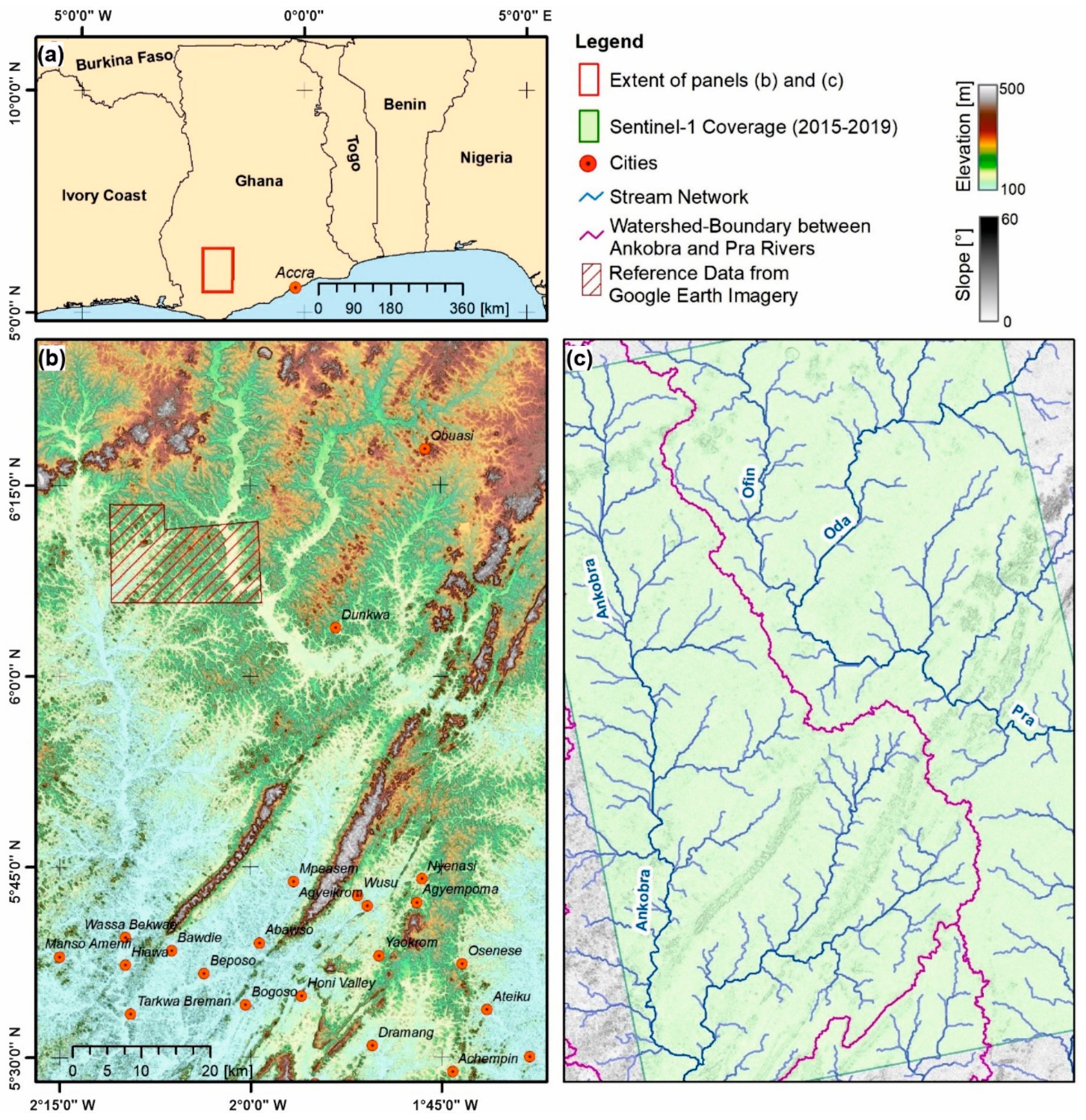
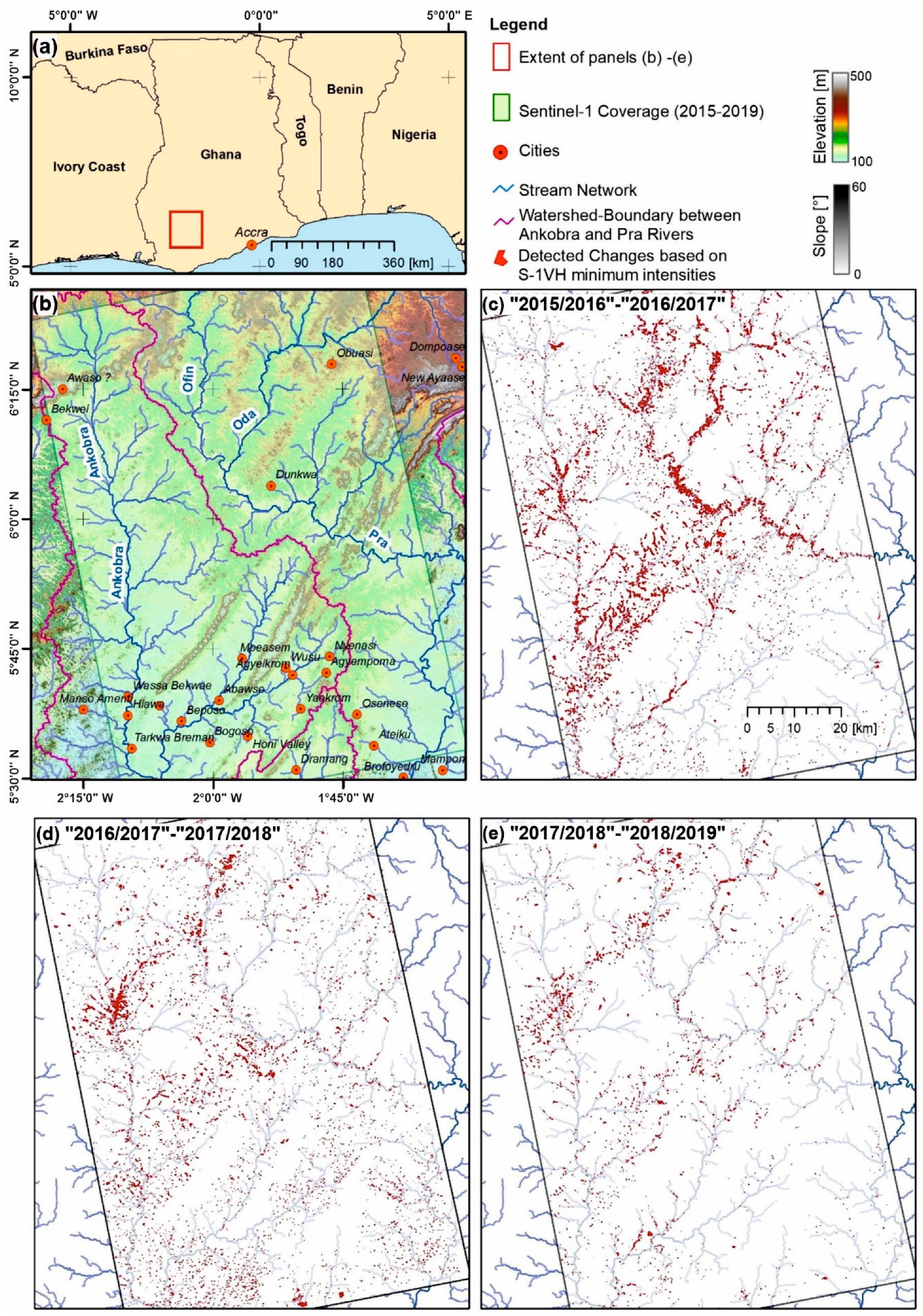
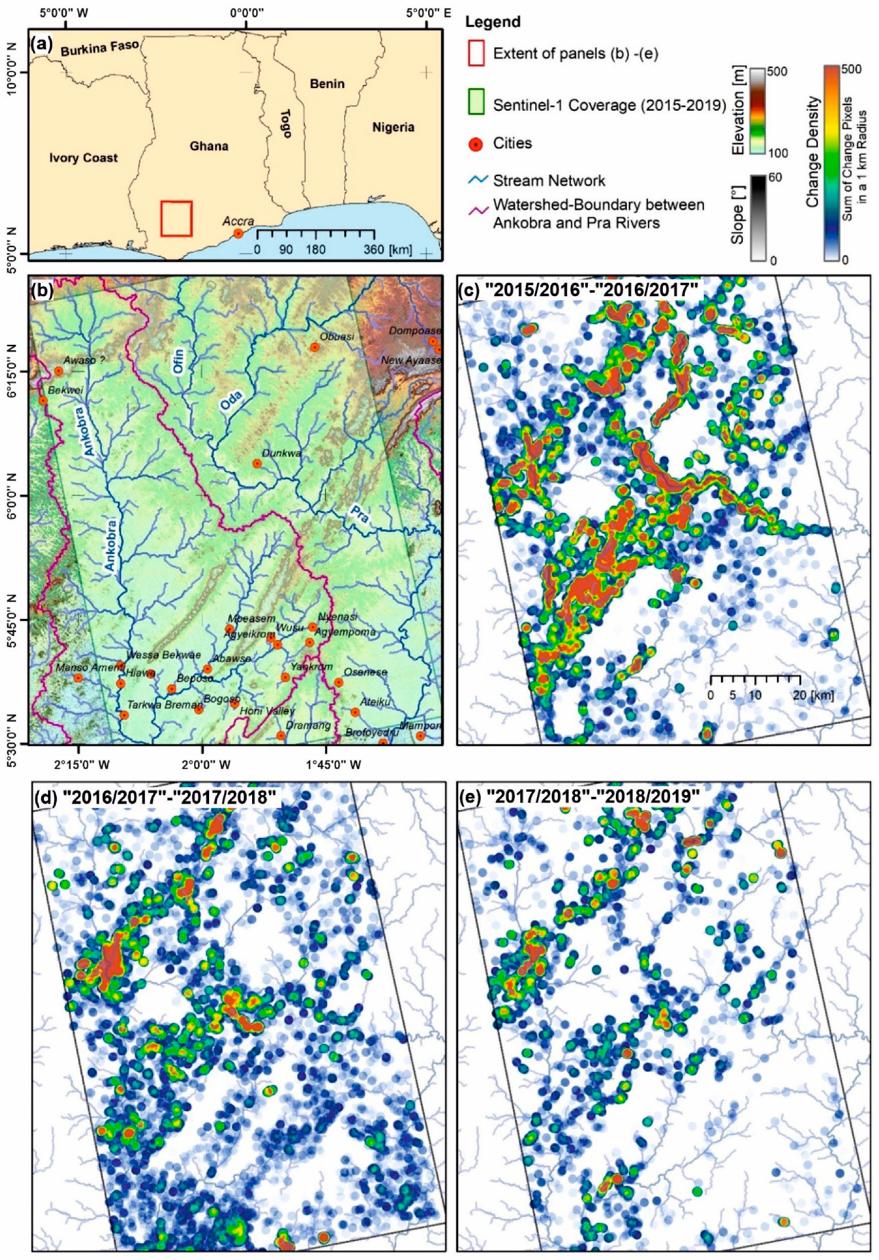
Access to this data is free and open, which makes them an ideal data source for data poor regions such as West Africa. The C-Band data of S-1 are suited for the characterization of spatiotemporal dynamics, i.e., identification of land cover changes over time, as they offer a large spatial coverage with a single acquisition and a temporal revisit of usually 12 days [26,27]. Time series data of S-1 were analyzed for a study area south of the city of Kumasi. The overall scope is to map and monitor the extent of small-scale mining activities along the Ankobra, Ofin, Oda, and Pra rivers in Ghana. Specifically, the study sought to answer the following research questions: (i) what is the suitability of C-Band Sentinel-1 data in monitoring illegal mining activities in South-Western Ghana, and (ii) what has been the temporal dynamics in the extent of illegal mining areas in South-Western Ghana between 2015 and 2019.

2. Materials and Methods

2.1. Study Area

The study area is located in South-Western Ghana and encompasses an area of 9071 km² (Figure 1). It overlaps three administrative regions (Ashanti, Central and Western South) which are the main regions in which industrially operated gold mines in the country are located [12]. Some of the worst affected municipalities and district assemblies such as Amansie West and Central, Wassa Amenfi East and Central, Wassa West, Upper Denkyira, Obuasi Municipal and Adansi North are located in, or overlap, the study area. Major rivers that drain the area, along which illegal mining takes place include Ankobra, Offin, Oda and Pra.

The largest settlement in the study area is the mining town of Obuasi, which is home to Ghana’s largest gold mine AngloGold Ashanti. Two other industrial mines that undertake surface mining are located northeast of Bogoso and west of Ayanfuri (Figure 1). The study area falls in the moist semi-deciduous forest agro-ecological zone of the country. Average annual temperature is about 26 °C. The agro-ecological zone is characterized by two distinct rainfall seasons: a dry season that spans from December to February and a wet season from March to November. Unlike temperature, precipitation is relatively variable within the study area. For example, from north to south, annual precipitation of prominent towns are 1450 mm (Obuasi), 1531 mm (Dunkwa) and 1682 mm (Bogoso) [28]. The study area is covered by both evergreen and deciduous forests. The latter lose their leaves for a short period of the year, whereupon new ones immediately begin to grow [29].

2.2. Data

2.2.1. Sentinel-1 Time Series

A total of 155 S-1 scenes covering the period 23 July 2015 to 9 April 2019 were downloaded from the Sentinel data hub (scihub.copernicus.eu) as Single-Look-Complex (SLC) products. The scenes were acquired in the Interferometric Wide Swath (IW) mode with VV and VH polarizations and were available in a 12-day interval. All datasets were acquired at 6:25 pm local time in the evening. Although all the datasets lie in the same relative orbit (number 45), there are slight differences in terms of location/extent. For example, for the period 20 November 2015 to 13 May 2017, a more northerly and southerly scene of one day each had to be used to ensure that the study area was completely covered. Consequently, the 155 scenes cover 117 unique days. Scenes acquired at the same data were mosaicked after the processing. However, not all scenes could finally be used in the analysis due to atmospheric effects that reduced the image quality (see Section 3.1). The data were processed using the Sentinel Applications Platform (SNAP) software (version 7.01.) (step.esa.int/main/toolboxes/snap/), IDL (version 8.7), and ENVI (version 5.5) (www.harrisgeospatial.com). The processing of the S-1 time series is illustrated in Figure 2 along with the general workflow of the approach. The processing included standard processing steps (i.e., Apply Orbit File, Split, Deburst, Calibration, Multilooking, Terrain Flattening, Boxcar Speckle Filter using a moving window of 5 by 5 pixels, and Terrain Correction). The data were projected to a common gird (World Geodetic System (WGS) 1984, Universal Transverse Mercator (UTM) Zone 30 North) with a pixel spacing of 20 by 20 m, which is not the best possible resolution achievable (approximately 12–15 m), but a compromise considering the speckle effect and the radiometric quality. The terrain corrected gamma nought intensities of the VV and VH channel were used in the subsequent analysis. From the full time series, temporal subsets were generated. These sets were defined as follows: “2015/2016” (July 2015 to June 2016), “2016/2017” (July 2016 to June 2017), “2017/2018” (July 2017 to June 2018), and “2018/2019” (July 2018 to April 2019). These “equal” periods were defined to allow comparison from one period to the other.

2.2.2. SRTM Digital Elevation Model

The 30 m resolution digital elevation model (DEM) from the Shuttle Radar Topographic Mission (SRTM) was downloaded from the Earth Explorer portal of the United States Geological Surveys (USGS) (earthexplorer.usgs.gov). The SRTM data was used to conduct hydrological/watershed analysis that can be used to locate activities of illegal miners in the study area in terms of hydrographical position (Figure 1 and Figure 2). The DEM underwent hydrographic modeling in ArcMap 10.6.1. The “Fill” function was applied during hydrographic pre-processing to remove sinks. Flow direction and flow accumulation were subsequently calculated. The channel network was deduced using a watershed size of >4 km². Using this channel network, the stream order of Shreve [30] was calculated for each line segment. This allows us to characterize detected activities in terms of stream order, e.g., if activities are found on small or large tributaries. Finally, the watersheds of the Ankobra and the Pra rivers were approximated by using the “Watershed” function and pour-points placed at the lower southern border of the study area.

2.2.3. Reference Data

Reference data were extracted from two sources including time-series land use/land cover data (LULC), and high-resolution Google Earth Imagery of a smaller area that was strongly affected by mining activity between 2015 and 2017. The LULC data, obtained for the nominal years 2006 and 2015, were derived from regional scale analysis by Gessner et al. [31] and Forkuor et al. (in preparation) based on multi-sensor satellite data. Both sources of reference data were used to identify changed and unchanged targets for the general scattering assessment and subsequent determination of thresholds for detecting mining activities (see Figure 2).

The high-resolution Google Earth images used as source of reference were acquired in February/April 2015 and May/December 2017 (Figure 3). These images clearly indicated mining activities along a small tributary of the Ankobra River in the western part of the study area, close to the town of Diaso. The reference data covered an area of approx. 19 by 14 km (266 km²) and 104 locations, affected by mining activity, were mapped based on visual image interpretation. On average, these polygons had a size of approximately 3.5 ha, while the smallest changed area that was mapped had a size of 0.5 ha (i.e., smaller areas than this were not considered). It was not possible to compile further meaningful and reliable high-resolution images of larger areas within test site. This was due to cloud cover and/or unsuited acquisition dates, e.g., most recent high-resolution images available in Google Earth date to 2015 and are, therefore, not useful for referencing of changes, as S-1 acquisition started in July 2015.

2.3. Change Detection

Change detection technique was used to map the extent of illegal mining along water bodies in the study area based on Sentinel-1 time-series data. The methodology is premised on the fact that analysis of SAR images acquired with the same acquisition geometry (i.e., same relative orbit) will reveal changed areas as having different scattering characteristics over time, while unchanged areas will have very similar scattering characteristics over time. Comparing the intensities between two sets, the variations in intensity of unchanged targets should be low and approximately in the order of ±1 dB, as reported by References [32,33]. Further, as the establishment of new mining areas usually infers a land cover change from vegetation to bare areas or water, the magnitude of the change in intensity is expected to be fairly high, exceeding the above mentioned 1 dB criteria. It is, therefore, reasonable to attribute significant differences in SAR intensities between two image periods to changes in land cover. In this regard, our methodology assumed that detected land cover changes along major rivers in the study area are induced by illegal mining activities, and the magnitude/extent of the change represents the area under illegal mining. The change detection methodology entailed four steps.

2.3.1. Sensitivity of Sentinel-1 Time-Series to Land Cover Changes

Sentinel-1 image time-series were analyzed to ascertain its suitability to detect changes in land cover in the study area. For each of the four temporal subsets defined in Section 2.2.1 and polarization channels (VV and VH), three time-series features were extracted along the temporal dimension of the time-series. These features were the minimum, mean, and maximum. To evaluate the sensitivity of Sentinel-1 data to land cover changes, the VV and VH scattering characteristics (histograms) of the time series features minimum, mean, and maximum were derived for two broad land cover classes: “water” and “agro-forest”. These two classes were selected because illegal mining activities in the study area usually cause a removal of vegetation and the creation of dug-outs or pools of water. Water is thus the dominant land cover after vegetation removal, between which there could be bare soil or vegetation. It is assumed that such changes in land cover (i.e., vegetation to water) will be highlighted in the time series features of S-1, as vegetation and water have different scattering characteristics and the received intensity from vegetation is usually higher than the intensity from water surfaces.

Reference information for the two LULC classes were extracted from existing LULC datasets of Gessner et al. (2015) and Forkuor et al. (in preparation) (see Section 2.3). The overall separability between the two classes offered by the respective time series features (i.e., minimum, mean, maximum) was investigated based on the extracted statistics of the classes and two metrics “distance” (DIST) and “similarity” (SIM) as defined by [34]. Both metrics quantify the distance/similarity between two probability functions (i.e., the histograms of the classes “water” and “agro-forest”). Higher values of DIST and lower values of SIM point to a better separation offered by the feature under investigation, e.g., how well the histograms of both classes separate in the VV mean intensity of set “2015/2016”. Therefore, the two metrics DIST and SIM enable a determination of the time series feature(s) that is/are most sensitivity to mining-induced land cover changes. Further, the class statistics indicate the expected magnitude and direction of changes e.g., when a land cover changes from “agro-forest” to “water” occurs.

2.3.2. Determination of Threshold for Detecting Changed and Unchanged Areas

The time series feature(s) (i.e., minimum, maximum, mean) identified as the most sensitive to land cover changes were further analyzed in order to find a threshold that is suited to identify/classify “changed” and “unchanged” areas in the S-1 time series features. First, changed and unchanged areas were mapped from high-resolution Google Earth Imagery. Visual interpretation was used to identify areas that had experience change due to mining activities between 2015 and 2017, as well as unchanged areas. Second, difference images between the time-series features of the temporal subsets “2015/2016” and “2016/2017” (i.e., the difference images of the VV/VH minimum/mean/maximum intensities) were derived. Based on an overlay of the difference images and the mapped “changed” and “unchanged” areas, histograms of the “changed” and “unchanged” areas were derived and analyzed to determine a suitable threshold for detecting mining-induced land cover change between the two temporal subsets (i.e., “2015/2016” and “2016/2017”).

Two approaches were tested to determine a threshold. The first is a supervised technique where the threshold is determined based on the intersection of the two histograms (i.e., the intensity value where both “changed” and “unchanged” classes show the same frequency). The second is an unsupervised methodology proposed by Otsu (1979), which iteratively seeks to minimize the interclass variance. The Otsu algorithm was directly applied using the difference images between the time-series features (i.e., no reference information on “changed” and “unchanged” areas is needed to compute the threshold).

Both approaches realize a simple form of binary image classification using a one-dimensional feature space and perform well if bimodal distributions are investigated [35], which was the case here. However, they do not necessarily identify the same threshold, which can provide an insight into the influence of changing thresholds in detecting mining-induced-changes. Additionally, the two metrics DIST and SIM were calculated to ensure that the feature offering the best separation is used in the subsequent step of classifying/mapping changes.

2.3.3. Detection of Illegal Mining Areas

Thresholds determined from the two approaches (i.e., histogram intersection and Otsu) (Section 2.3.2) were applied to difference images computed from the temporal subsets to identify changed and unchanged areas. Difference images were computed for three periods as follows: Period 1: “2015/2016”–“2016/2017”, Period 2: “2016/2017”–“2017/2018”, and Period 3: “2017/2018”–“2018/2019”. The application of the threshold values to the difference maps resulted in multiple change/unchanged binary maps which were subsequently validated using reference data. Prior to this validation, a majority filter with a moving window size of 5 by 5 pixels was applied in the post-classification in order to remove isolated single pixels.

2.3.4. Accuracy Assessment and Analysis

For Period 1 (“2015/2016”–“2016/2017”), the change/no-change maps generated (based on threshold, polarization, time-series feature) were validated using reference data in order to assess the accuracy of the change detection and to indicate the most suited time series feature and polarization. Reference data of changed areas were derived from Google Earth Imagery (see Section 2.3) and formed the basis of this assessment. Producer’s and user’s accuracies of the changed class, as defined by Congalton and Green [36], were computed. In addition, errors of omission and commission were computed and presented. As several change/no-change maps were produced (i.e., for each polarization, time series feature and threshold), the accuracy assessments provided the basis for selecting the final map for estimating the temporal evolution of illegal mining area extent in the study area. Finally, the spatial pattern and temporal evolution of the changes were analyzed, also in relation to the stream order, which was derived from the SRTM DEM and linked with the classification results via a spatial join in ArcMap (10.6.1).

3. Results

3.1. Atmospheric Effects on Sentinel-1 Data

Our analysis revealed that a significant portion of the investigated S-1 data showed locally-restricted patches of strong local decrease in backscatter intensity in the order >−10 dB compared to the long-term mean intensity. Such areas (approx. 20–50 km² in size) of decreased intensity were found over the entire imaging area and did not show a specific spatial distribution or pattern (Figure 4). Further, these patches are found in single scenes only (i.e., not in consecutive scenes). The shapes of the patches are diffuse and borders are not clearly distinguishable (Figure 4). A total of 29, out of 117 (ca. 25%), scenes showed this effect and accordingly these scenes were not used in subsequent analyses. While no such patches were found in the 29 scenes acquired in August, in almost two thirds (7 out of 11) of the scenes acquired in March such patches were found. In October, half of the downloaded S-1 images (5 out of 10) were removed from the subsequent analyses. May and November were above average with three scenes affected, while in the other months only one or two scenes were affected. With regard to the annual distribution of corrupted images, the years 2015 to 2017 had between 25 to 32% of images affected by atmospheric effects. The year 2018 was less affected, with only 13% of scenes being unusable. The year 2019 was the most impacted, with a maximum 44% of scenes eliminated due to these effects.

3.2. Feature Selection and Threshold Definition

The separability offered by the time series features minimum, mean, and maximum was estimated for both polarization channels for the set “2016/2017” using the “water” and “agro-forest” classes from the two LULC classifications (see Figure 5). The minimum and mean features showed very clear separation of the values of both classes (i.e., water and agro-forest), while maximum features (at VV and VH) showed less separability but rather increased overlap of classes’ frequency distributions.

These findings are also supported by the DIST and SIM metrics (

Table 1. Results of the distance (DIST) and similarity (SIM) metrics of classes “water” and “agro-forest” for the investigated time series features minimum (MIN), maximum (MAX), mean (MEAN) and for both polarization channels (VV/VH) (see Figure 6). The two metrics quantify the separation between the frequency distributions of both classes. Higher values in DIST and lower values in SIM point to a better separation offered by the feature under observation.

Feature	DIST	SIM
VH Min	1.998	0.0009
VH Mean	1.996	0.0017
VH Max	1.817	0.0912
VV Min	1.998	0.0007
VV Mean	1.998	0.0009
VV Max	1.686	0.1566

). Lowest SIM and highest DIST values were obtained for the minimum features, followed by the mean features. The maximum features showed higher SIM and lower DIST values. Both polarizations performed similar and values of the metrics were nearly the same for both VV and VH. Therefore, the minimum and mean features of both polarizations offered a better separation of the classes “water” and “agro-forest” compared to the maximum features, while there is no clear difference in performance between VV and VH. Consequently, the minimum and mean features were found to be more sensitive to mining-induced changes than the maximum.

Difference images of the VV/VH minimum/mean intensities between periods “2015/2016” and “2016/2017” were used to derive thresholds for detecting changes in illegal mining areas. Results of this analysis are shown in Figure 6 and

Table 2. Results of the distance (DIST) and similarity (SIM) metrics for classes “unchanged” and “changed” for time series features minimum (MIN) and mean (MEAN) in both polarization channels (VV/VH). The two metrics quantify the separation between the frequency distributions of both classes (see Figure 7). Higher DIST values and lower SIM values indicate a better separation between the classes. The last two columns show the thresholds estimated by the histogram intersection and by the Otsu Algorithm.

Feature	DIST	SIM	Threshold (Histo. Intersection)	Threshold (Otsu Algorithm)
Difference VH Min	1.83	0.084	+1.65 dB	+2.78 dB
Difference VH Mean	1.85	0.071	+1.22 dB	+2.30 dB
Difference VV Min	1.81	0.093	+1.62 dB	+2.34 dB
Difference VV Mean	1.85	0.071	+1.46 dB	+1.99 dB

. The high-resolution Google Earth images (see Figure 3), available for a smaller portion of the study area, were analyzed to identify targets (“changed”/“unchanged”), which served as the basis for evaluating the time series features minimum and mean and determining a threshold that represents/indicates change. Figure 6 shows that changed areas generally had higher difference in intensity and variance than unchanged areas in both VV and VH polarizations. Analysis of the histograms indicate similarities in the statistics derived from the minimum and mean difference in intensity for both changed and unchanged areas. For example, in the case of changed areas, an average value of +4.6 dB (standard deviation of 2.3 dB) is observed for VV minimum and a corresponding value of +4.1 dB (standard deviation of 1.8 dB) was observed for VV mean. Corresponding average values of unchanged areas are +0.01 dB (VV minimum) and +0.32 dB (VV mean), while standard deviations are 0.88 dB (VV minimum) and 0.51 dB (VV mean).

Similar observations were made for VH minimum and mean intensity plots. For changed areas an average value of +5.3 dB (standard deviation of 2.3 dB) was observed in the VH minimum and an average of +4.7 dB (standard deviation of 2.1 dB) was observed in the VH mean intensity. Corresponding values for unchanged areas are −0.01 dB (VH minimum) and +0.08 dB (VH mean), while standard deviations are 0.82 dB (VH minimum) and 0.47 dB (VH mean). This indicates that changed and unchanged areas exhibit similar characteristics in both VV and VH polarizations irrespective of the statistic (minimum or mean) being used to detect difference in intensity from one period to the other. Nonetheless, in all cases, changed areas have a higher variance and intensity difference than unchanged areas.

Table 2 presents the threshold values for detecting changed areas from the statistics (minimum and mean), as determined from the intersection of the respective histograms of changed and unchanged areas/targets (Figure 6) as well as from the Otsu algorithm. For VH polarization, the histogram intersection analysis revealed a threshold value of +1.22 dB based on the mean difference in intensity and a value of +1.65 dB for the minimum difference in intensity. The corresponding threshold values identified by the Otsu algorithm were generally higher: +2.8 dB (VH minimum) and +2.30 dB (VH mean). For VV polarization similar thresholds as in the VH were found in the histogram intersection, which were +1.62 dB for the minimum difference in intensity and +1.46 dB for mean difference in intensity. The corresponding threshold values identified by the Otsu algorithm were again higher, i.e., +2.34 dB (VV minimum) and +1.99 dB (VV mean). Compared to the DIST and SIM metrics, it was found that highest values in DIST and lowest values in SIM were obtained by mean features in both polarizations. On the other hand, the minimum features showed very small differences. Again, no meaningful difference between the VH and VV polarization was found, with both exhibiting very similar values.

Figure 7 shows a subset of the mean and minimum features of VV and VH polarization for periods “2015/2016” and “2016/2017”, the resulting difference images, and the Google Earth Imagery. The visual comparison and interpretation indicates that mining activities can be detected with positive intensity difference values of approximately >+2 dB in both time series features. While changed areas in the upper part of the subset were clearly indicated by significant intensity differences, some areas in the lower part of the subset were not indicated.

3.3. Change Detection

Using the thresholds identified in Table 2, change maps (i.e., binary classifications of “unchanged” and “changed”) were generated for all three periods (i.e., for “2015/2016”–“2016/2017”, “2016/2017”–“2017/2018”, and “2017/2018”–“2018/2019”). This operation is illustrated in Figure 8 for the difference in VH minimum intensities and for thresholds identified by the histogram intersection (threshold = +1.65 dB) and the Otsu algorithm (threshold = +2.78 dB). Comparing the resulting classifications, it is clear that less “changed” areas were identified by the Otsu algorithm threshold, as a higher threshold yielded a stricter prerequisite for classification of “changed” areas. Further, it is clearly visible in the imagery that in Period 1 much more changed areas were identified compared to the subsequent periods. Subsequently, accuracy assessment was carried out in order to judge, which combination of polarization, feature and thresholds finally offered the best classification accuracy based on the reference data. This assessment (

Table 3. Accuracy assessments of class “changed” based on the differences between the VV/VH mean/minimum intensities between sets “2015/2016” and “2016/2017” (Period 1) (see Figure 9), the thresholds identified in Table 2 and reference data generated from the Google Earth Imagery (see Figure 1 and Figure 8). Note: Prod. Acc. = Producer Accuracy, User Acc. = User Accuracy.

Feature	Threshold [dB]	Commission [%]	Omission [%]	Prod. Acc. [%]	User Acc. [%]
VH minimum intensities “2015/2016”–“2016/2017”	+1.65	27.61	15.11	84.89	72.39
VH minimum intensities “2015/2016”–“2016/2017”	+2.78	15.10	31.03	68.97	84.90
VH mean intensities “2015/2016”–“2016/2017”	+1.22	16.45	22.90	77.10	83.55
VH mean intensities “2015/2016”–“2016/2017”	+2.30	7.42	53.52	46.48	92.58
VV minimum intensities “2015/2016”–“2016/2017”	+1.62	27.84	28.52	71.48	72.16
VV minimum intensities “2015/2016”–“2016/2017”	+2.34	14.65	42.75	57.25	85.35
VV mean intensities “2015/2016”–“2016/2017”	+1.46	17.02	44.85	55.15	82.98
VV mean intensities “2015/2016”–“2016/2017”	+1.99	10.31	62.87	37.13	89.69

) was done for class “changed” based on the differences between the VV/VH mean/minimum intensities between periods “2015/2016” and “2016/2017” (Period 1), the two thresholds identified in Table 2 and the reference data information taken from the Google Earth Imagery (Figure 3).

The assessment (Table 3) indicates that most accurate classifications (i.e., highest user accuracy (UA) and producer accuracy (PA)) were achieved in VH polarization using the minimum (UA = 72.39%, PA = 84.89%) or mean (UA = 83.55%, PA = 77.10%) features and the threshold identified by the histogram intersection. The stricter (higher) threshold values of the Otsu algorithm generally lead to higher UAs at the expense of PA (i.e., they are indicated by lower commission but higher omission). Therefore, best UA of 92.58% is found for the VH mean intensities and the threshold value of the Otsu algorithm; however, this classification also shows the second lowest PA with 46.48%, lowest PA with 37.13 % is observed for VV mean intensities and the threshold identified by the Otsu algorithm. Based on these results, the final classifications were processed using the VH polarization, the minimum feature and the threshold identified via the histogram intersection. The results are shown in Figure 9. The classifications are further displayed as density maps. These were processed by summing up changed pixels within a radius of 1 km (Figure 10).

The results indicate that land cover changes in Period 1 were frequently found along the Ofin, Oda and Pra Rivers, as well as along the Ankobra River and its tributaries in the southwestern part of the study area. The change patterns were clearly oriented and followed the course of the channel network for most locations. Generally, less land cover changes were found in Period 2. Here, the highest density of changes were found along the Ofin River and the Ankobra River south of Bekwai. Similarly, changes in Period 3 were less frequent compared to the preceding periods and highest density was found along the Ofin River and the Ankobra River south of Bekwai.

These observations are summarized in Figure 11. The total changed area reduced over time from about 102 km² (“2015/2016” and “2016/2017”), to 60 km² (“2016/2017” and “2017/2018”), to 33 km² (“2017/2018” and “2018/2019”). This means that the changed areas halved from first to second, and from second to third periods. Along with this, it was found that the average Shreve stream order of the changed areas reduced over time (Figure 11b), which indicates that activities moved to smaller tributaries in the course of time. This decrease was strongest from first to second period, while changes in Shreve order were lower between second and third periods. Considering the spatial patterns of changed areas (Figure 9 and Figure 10) this was related to fewer changes observed along the Oda and Pra Rivers, as these river systems were characterized by high values of the Shreve stream order.

4. Discussion

4.1. Susceptibility of Sentinel-1 data to Cloud Cover

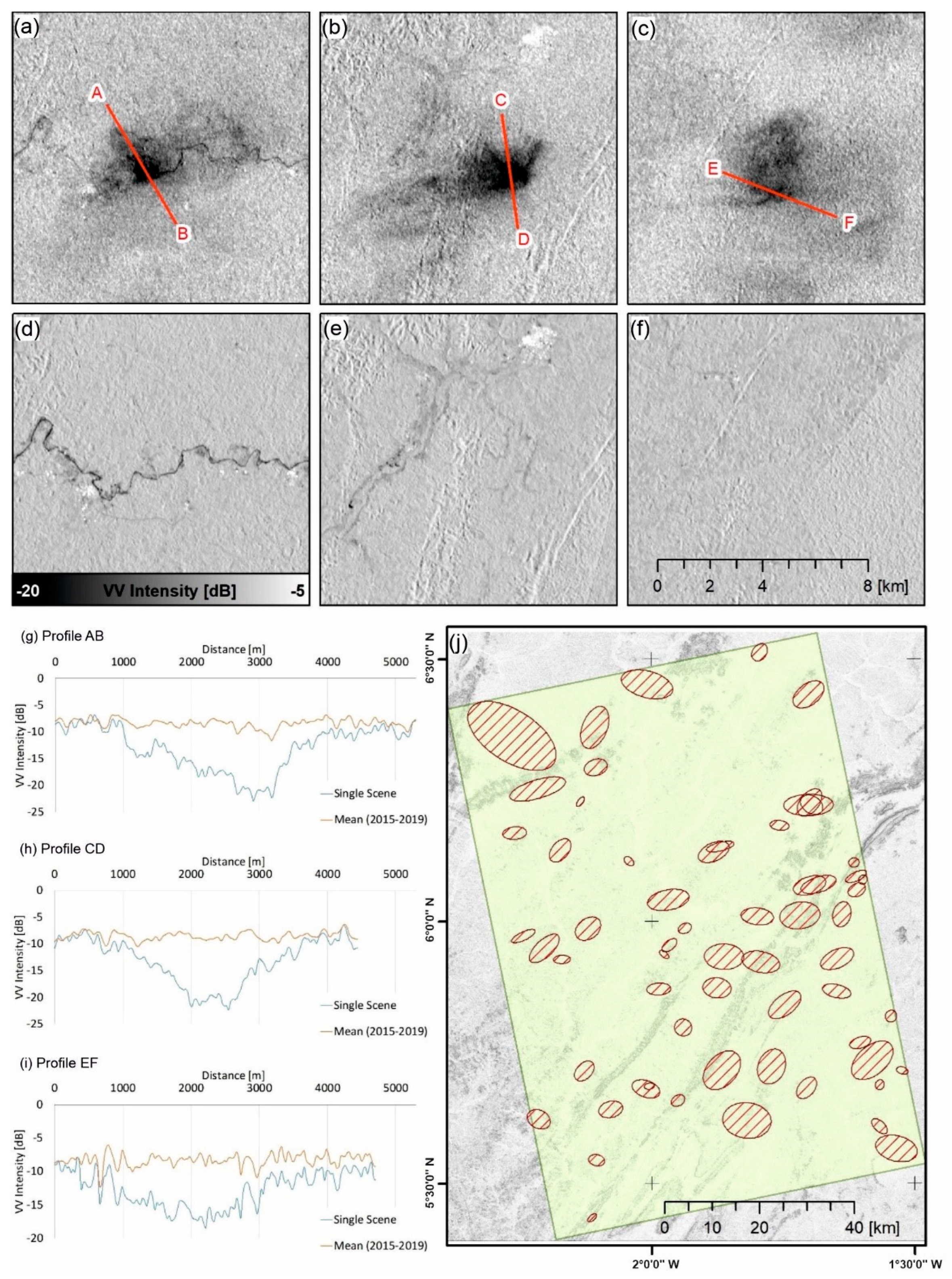
The analysis revealed that a significant portion of the S-1 data were affected by atmospheric effects, typical for SAR acquisitions taken over cloud-prone regions [37]. Affected areas were characterized by a strong local decrease in the backscatter intensity of single scenes compared to the long-term mean intensity of the time-series. It is assumed that the strong lowering of the backscatter was caused by large convection cells and heavy rainfall events that are typical of the study region. However, this effect is usually more frequently observed at short wavelengths (e.g., X-Band) [37,38], while longer wavelength such as C- and L-Bands are usually less affected due to the larger penetration depth. Nevertheless, Alpers et al. 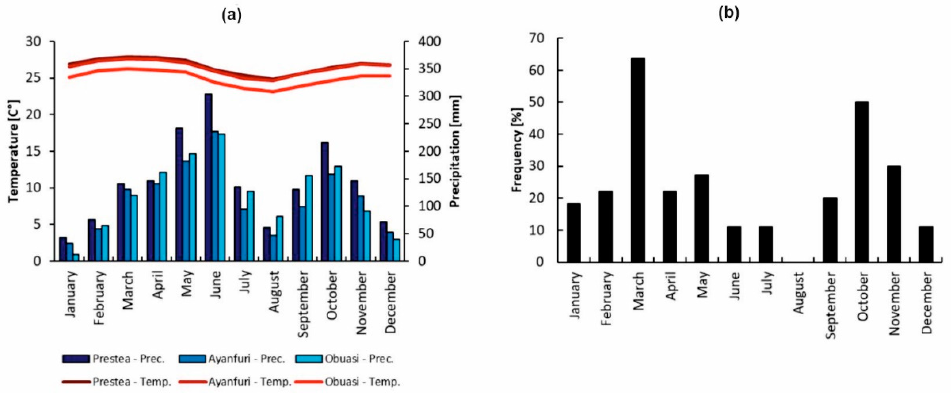[38] pointed out that high precipitation amounts of several tens of millimeters per hour can cause a significant lowering of the backscattering intensity, even at C-Band. The S-1 scenes acquired in March or October (i.e., during the rainy seasons) were more frequently affected than scenes acquired in other months (Figure 12). The first (major) season begins in March, while the second (minor) usually starts in September [39]. Especially at the beginning of the first season and the end of the second season (i.e., the months of March/April and October/November) convective rainfalls, such as strong local rainstorms and squall lines (i.e., line of thunderstorms), are frequently observed in the area. These events are characterized by intensive and short-lasting rainfalls, which can reach precipitation amounts of more than 30 mm/h within the first half hour [39]. Friesen [40] noted that rainstorms are short lasting (1–2 h) and stationary systems that usually affect rather small areas of approx. 20–50 km²; a size that fits well with the average extent of the affected areas. Further, the rainstorm events occur most frequently in the evening due to their convective nature and this is also the time at which the S-1 images are acquired.

4.2. Change Detection and Monitoring of Illegal Mining

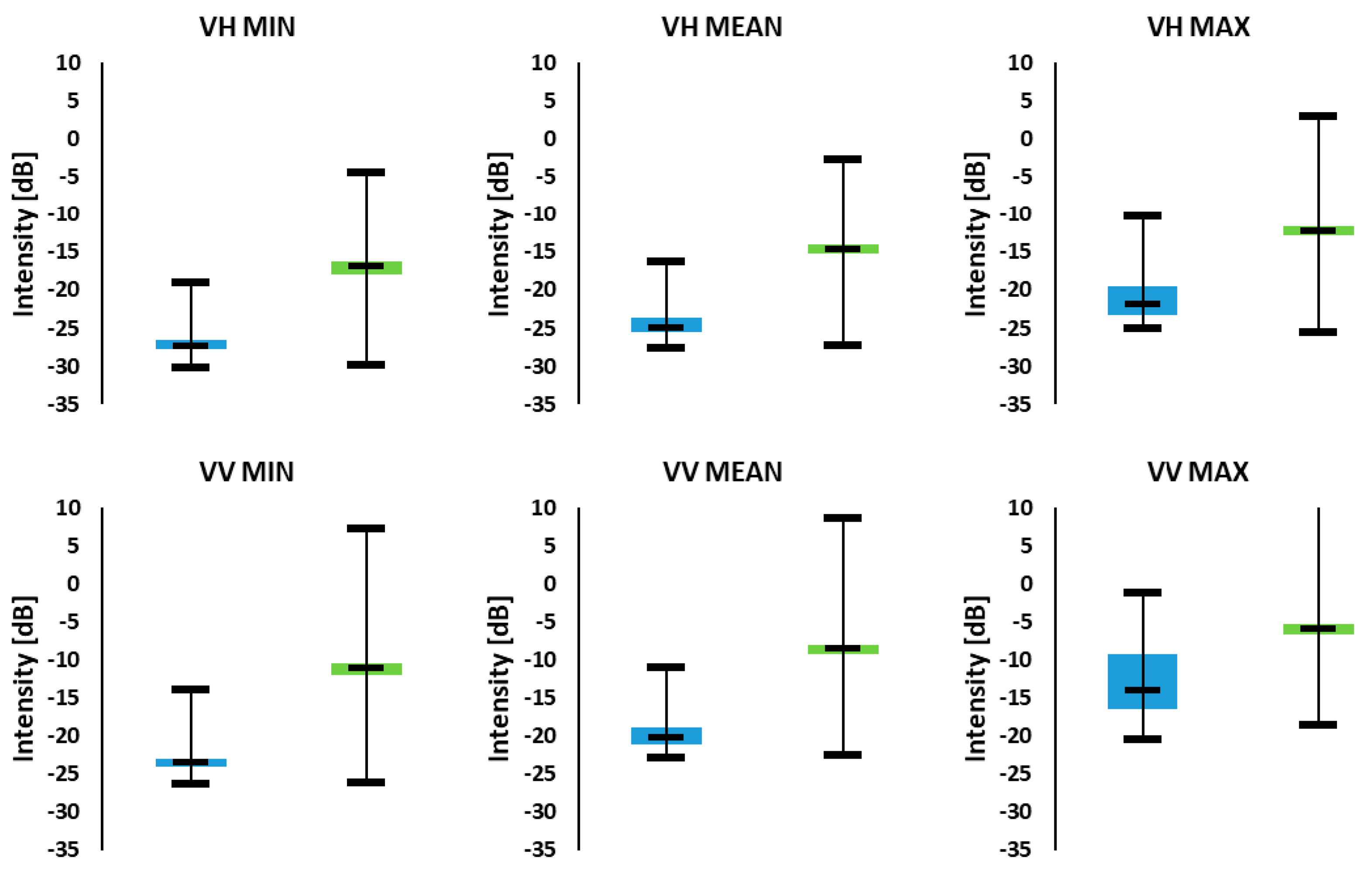
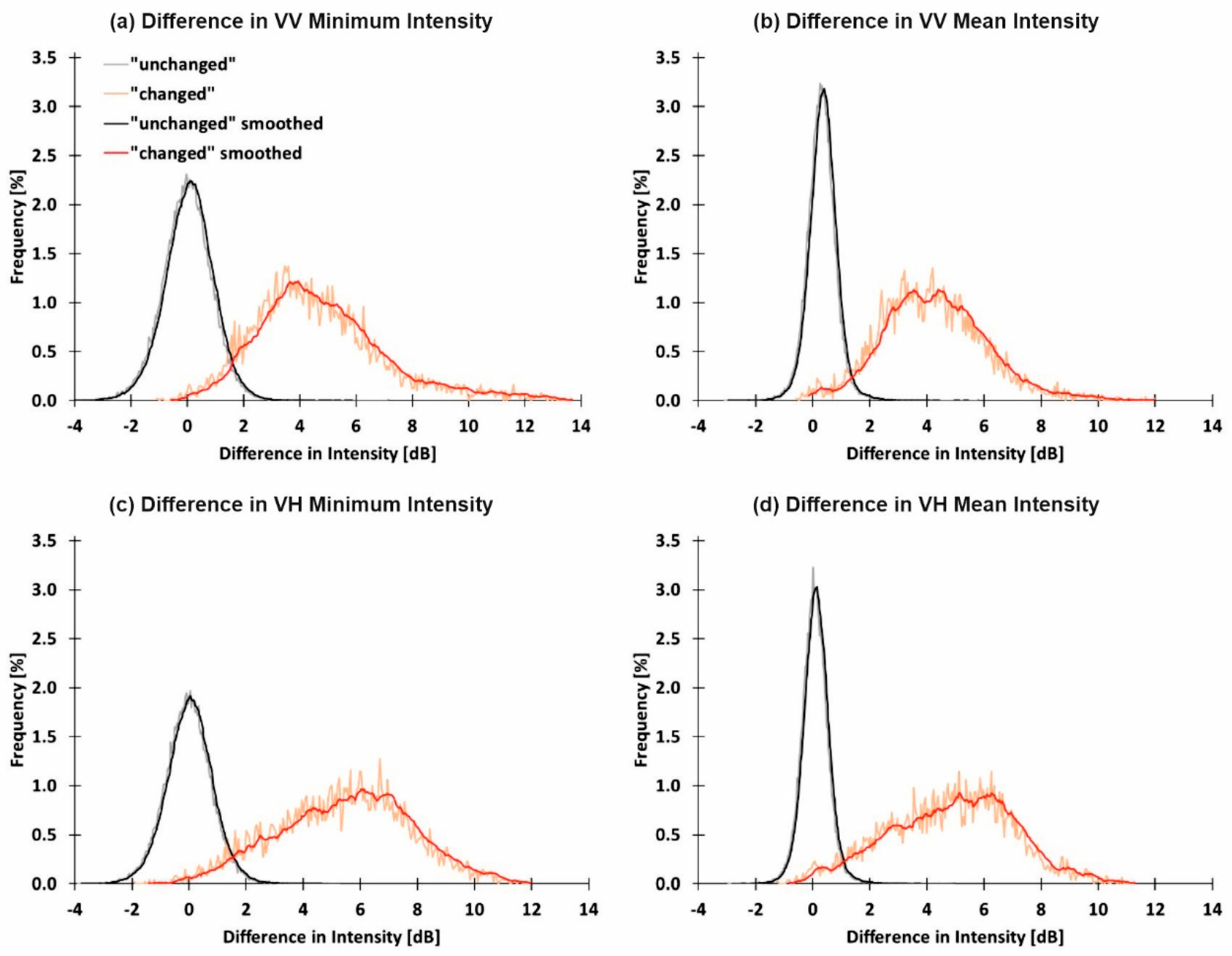
This study employed a change detection method that was based on the generation of binary changed/unchanged masks using single thresholds, estimated via histogram analysis and the Otsu algorithm. The analyses were based on S-1 time-series features (i.e., minimum, mean and maximum backscattering intensity observed within one year), as they offered the following advantages compared to the analysis of single scenes: (i) speckle is reduced due to the temporal averaging, (ii) seasonal effects are averaged and compensated and thus do not appear as change areas in the classification result, (iii) the temporal features still preserve most important information on the backscatter characteristics and therefore on potential LULC changes. Due to the high signal stability of S-1 [32,33] it was expected that significant changes in the average backscattering intensities (approx. > ±1 dB) between the time series features of two temporal periods can be attributed to changes in land cover.

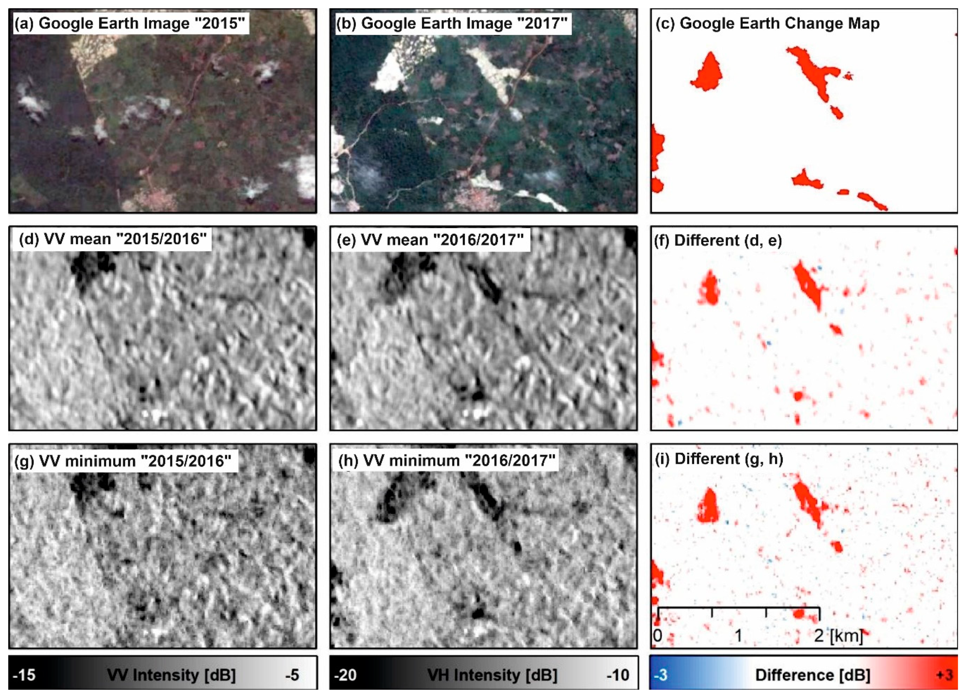
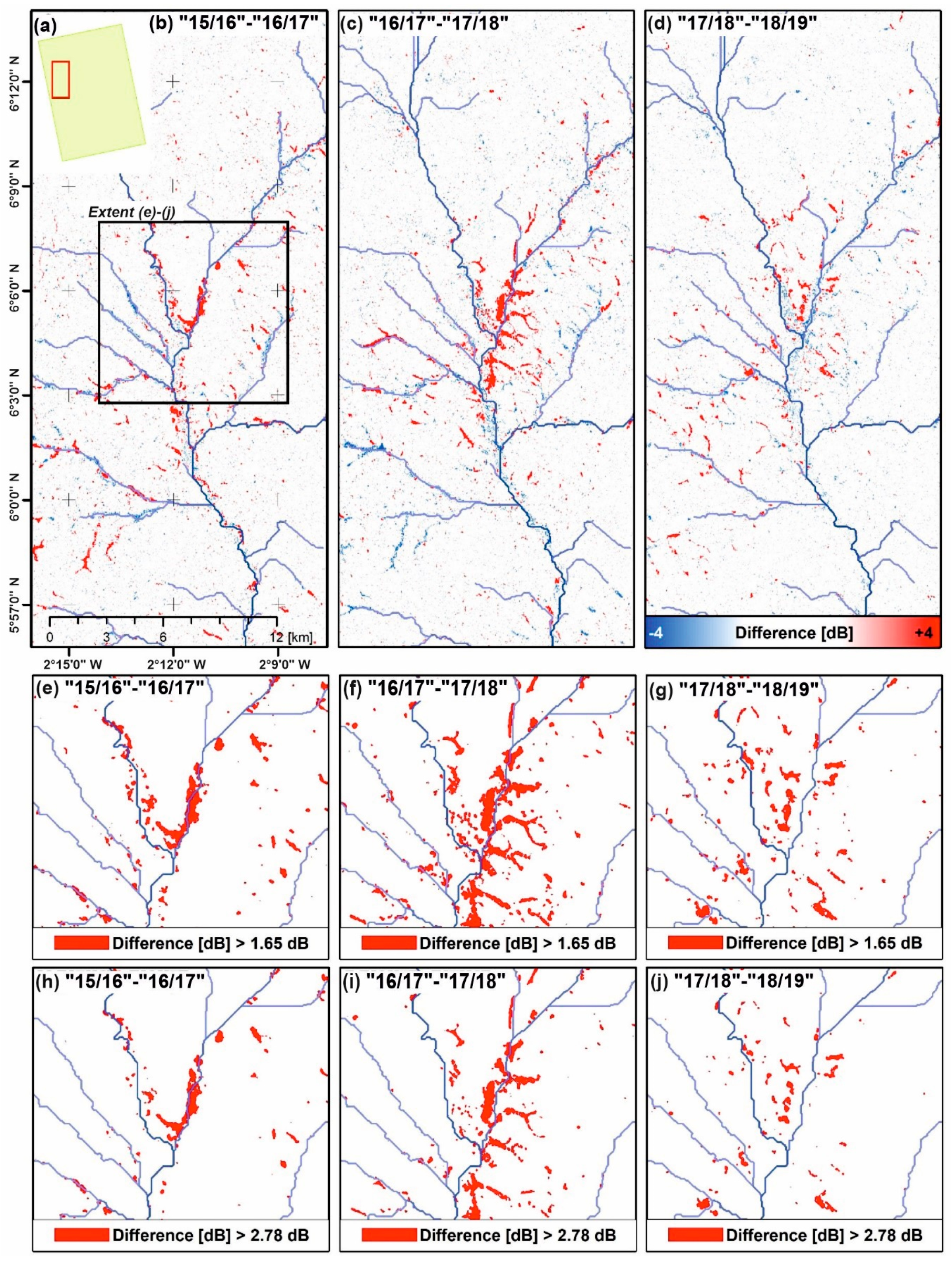
As pointed out, mining activities in the study area usually cause a removal of vegetation and the creation of dug-outs. The analysis pointed out that LULC changes associated with mining activities were indicated by changes in both VV and VH intensities of +1.65 dB or higher (i.e., threshold estimated for VH minimum via histogram intersection), this compares well with the expected direction and magnitude of a land cover change from vegetation to water/bare soil. On the other hand, unchanged areas showed average values around ±0 dB and standard deviations less than 0.9 dB for both polarizations and for all time series features. This observation is in line with results proposed by References [31,32]. Note in this context that the design of the approach inferred that only new sites could be detected, e.g., no information on the activity of already established sites or their abandonment was provided.

The analysis of the distance metrics (SIM and DIST), as well as the accuracy assessments conducted for Period 1 and for a smaller subset of the study area, showed that VV and VH polarization perform similar in change detection. However, the VH polarization achieved better classification accuracies, which might be attributed to the higher sensitivity of VH polarization to volume scattering processes. This sensitivity in turn leads to a better separation of water and vegetation classes in the feature space, compared to the VV polarization. Scattering from water is characterized by very low volume scattering contribution, whereas the presence of vegetation causes significantly higher volume scattering contributions and intensities at C-Band [41,42].

Among the investigated time series features, the minimum feature performed better than the mean or the maximum feature. This is reasonable, as the minimum feature is sensitive to any changes in backscattering within the period, as just the lowest intensity value observed is displayed in this feature. Due to this fact, it was of high importance to screen and remove datasets that are affected by atmospheric conditions (i.e., clouds), as they might cause false detections. Conversely, the mean feature is dependent on the time at which the changes occur, as all intensity values of the entire period are averaged, therefore changes that occur at the end of the observation period are more difficult to detect.

It is clear that the temporal integration and the analysis of time series features has drawbacks. First, no information on the exact timing of the change is provided beside the year/period. Second, the approach is not suited to the dynamic detection of new illegal mining areas, as the approach essentially requires longer observation periods to generate the time series features. These limitations also infer that small and short-lasting changes are unlikely to be detected, also considering the spatial resolution of the S-1 data. Since this study focused on detecting inter-annual changes in rather large-scale illegal mining activities in the past, it is expected that the stated drawbacks did not have a significant effect on our results.

In this study, the thresholds for generating the binary changed/unchanged masks were estimated using a supervised (histogram intersection) and unsupervised (Otsu algorithm) approach. Both approaches showed acceptable to good classification accuracies, which were ca. 68% (Prod. Acc.) and 83% (User Acc.) for the threshold estimated via the Otsu algorithm and ca. 84% (Prod. Acc.) and 72% (User. Acc.) for the threshold estimated via the histogram intersection. Higher thresholds values were generally observed via the Otsu algorithm, which resulted in higher user but lower producer accuracies. This means that higher threshold values result in more strict and conservative estimates and have fewer false alarms at the expense of more missed detections. Higher user accuracy in turn might be a prerequisite for actual ground validation and legal actions and thus desired in an operational context.

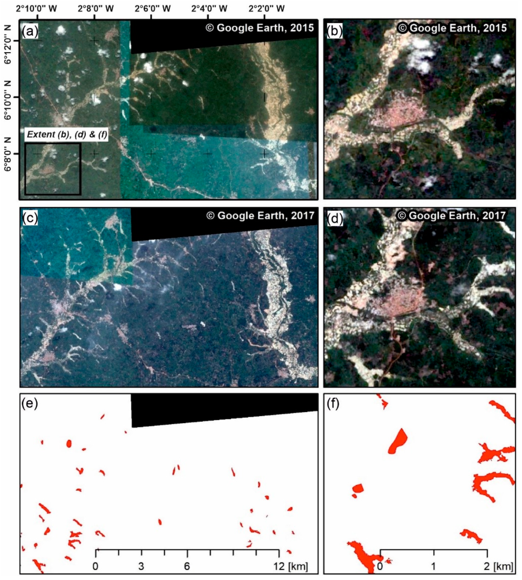
A challenge of this study was the quantity and extent of the reference data. As pointed out, the results were validated for a smaller region using high-resolution Google Earth Imagery. Mining activities can be detected on these imagery with a high level of confidence. However, due to persistent cloud cover, only few images were available that (i) covered a sufficiently large area affected by mining activities and (ii) the period of acquisition corresponded to the S-1 observation periods making them suitable for validation. Consequently, only few images provided a useful and reliable reference that was suited to assess the classification accuracies provided by the unsupervised and supervised binary classifications. In this regard, upcoming studies should compile more suited high-resolution optical space-borne imagery, also from commercial sources, e.g., the archive of the Planet satellites (planet.com). Having more high-quality reference data will allow for a more comprehensive classification and referencing, e.g., also for the most recent observation periods. On the other hand, future studies can embark on an extensive field campaign (including historical land use interviews) to generate more reference data for validation. Considering the increased observation frequency of optical space-borne systems (e.g., due to the operation of Sentinel-2), it might also be possible to fuse SAR and optical data in the classification process in order to enhance the classification accuracies, to increase the sensitivity of the detection and the spatial resolution of the classification result.

The presented approach does not require a comprehensive processing and therefore it can be repeated by using the Ground Range Detected (GRD) products of Sentinel-1. These products require less disk space, are already partially radiometrically corrected and the processing of sigma or gamma nought requires less processing steps, compared to the SLC products. Further, it is suggested to run the approach using cloud-processing facilities such as the Google Earth Engine (GEE) (earthengine.google.com) [43]. GEE already offers the necessary infrastructure to assess the S-1 archive (i.e., the GRD products are available) and to process time series features from a stack of S-1 images. This in turn will save the download and processing of large amounts of S-1 data and will provide analyses ready data. However, the issue that S-1 data are affected by atmospheric conditions (i.e., clouds) must be addressed, as patches of low backscattering will manifest in the minimum time series feature. Therefore, other metrics, e.g., such as the analyses of lower quantile values instead of the minimum, should be investigated as a cloud-based processing strategy is not suited to the manual selection and removal of individual scenes.

4.3. Trend in the Extent of Illegal Mining Areas between 2015 and 2019

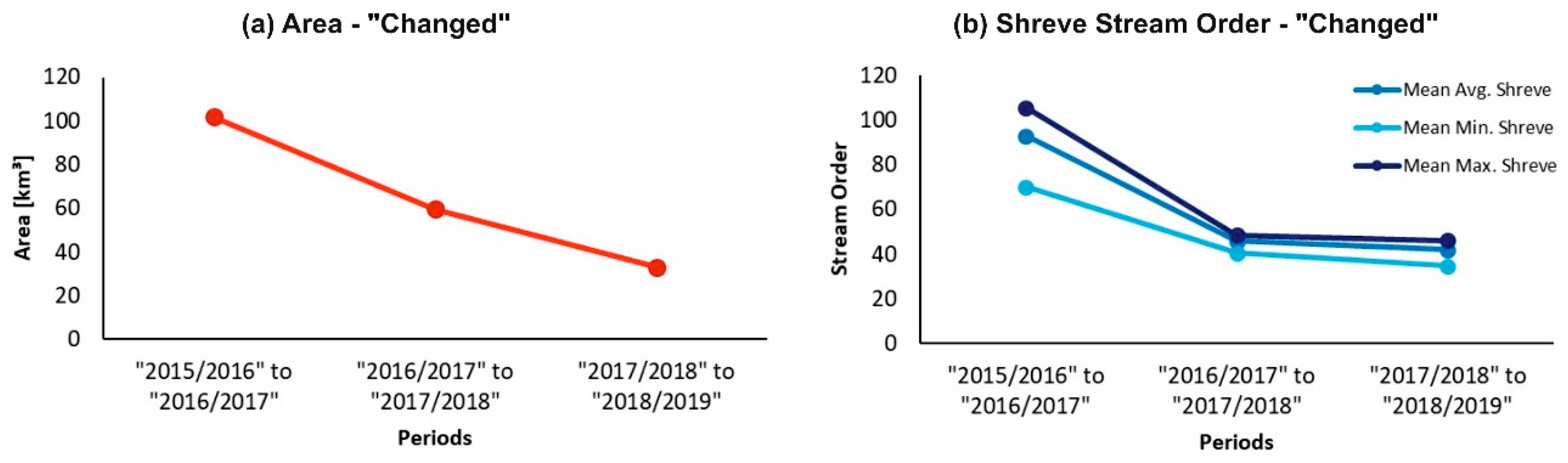
Our results showed a decreasing trend in the extent of illegal mining in the study area from 102 km² in Period 1 (2015/2016–2016/2017) to 60 km² and 33 km² in periods 2 (2016/2017–2017/2018) and 3 (2017/2018–2018/2019), respectively. Despite its widespread practice and resultant degradation and pollution, very few studies have used remote sensing data to quantify changes (over a period) in the extent of illegal mining activities in the country. This is principally attributable to excessive cloud cover in the southern part of Ghana where illegal mining mostly takes place, and the difficulty in obtaining usable optical images. Owusu-Nimo et al. [44] mapped and analyzed the spatial distribution patterns of artisanal small-scale gold mining in the Western region of Ghana, but did not use satellite imagery nor quantified the extent/area of the activity in the region. They generally mapped galamsey sites as points using field-based surveys and found a total of 911 galamsey sightings comprising of 7470 individual operations in 312 communities across 11 municipal and district assemblies in Western region. Out of 11 districts, they found three as the galamsey hotspot districts: Tarkwa Nsuaem (294 sightings), Amenfi East (223 sightings) and Prestea Huni Valley Districts (156 sightings). Two out of these three hotspot districts fall within our study area. Awotwi et al. [45] conducted a general land use and land cover mapping in the Pra river basin using a time-series of Landsat images acquired between 1986 and 2016. They noted an increase of 10.62% in the extent of mining areas between 2004 and 2008, and 304% between 2004 and 2016. Other studies also inferred increases in the extent of mining areas based on general land use and land cover analysis based on satellite imagery [20,46].

Snapir et al. [21] is the only study we have found that had a specific focus on assessing the extent of illegal mining sites between 2011 and 2015 using optical satellite imagery. For a subset of their study area (change area), they found that the extent of illegal mining areas tripled between 2011 and 2015, increasing from 109.07 km² in 2011 to 232.82 km² and 366.96 km² in 2013 and 2015, respectively. Although the area and period investigated are not the same as that of this study’s, a note-worthy difference in their results compared to ours is the trend in the extent of illegal mining areas, i.e., increasing trend in Snapir et al. [21] and decreasing trend in this study. Two possible reasons for this variance can be discussed. First, as alluded by Snapir et al. [21], their approach did not differentiate between active and abandoned pits or mining areas. Thus, the area detected in, for example 2013, could be a summation of abandoned pits from 2011 and active/new pits that opened in 2013. Similarly, active/new pits in 2015 would add up to those of 2011 and 2013 to indicate a much larger extent compared to previous years. The approach adopted in this study, however, detects mining-induced changes from one period to the other. Thus, the detected changes at Period 2, relative to Period 1, can be considered as new illegal mining areas that opened in the period under analysis. In this sense, when areas mapped in, for example, Period 1 are added to the area of detected change in Period 2, there would be an overall increase in the extent of illegal mining areas at Period 2. When analyzed this way, our results will indicate an increasing trend in the extent of illegal mining areas as 102 km², 162 km² and 195 km² for Periods 1, 2 and 3, respectively.

The second possible reason for the observed difference in trends, specifically the decreasing trend in our results (with respect to new illegal mining areas), is the government’s efforts to sanitize the small-scale mining sector and reduce illegal mining activities in the country. Although governmental effort to curb the menace started in 2013 with the establishment of an inter-ministerial task force, efforts from 2017 seem to have been more effective. These efforts include: (i) a six-month ban on all small-scale mining activities (even including licensed operators) and seizure of equipment, (ii) suspension of the issuance of licenses for small-scale mining, (iii) setting up of a Multilateral Mining Integrated Project (MMIP) to enact more stringent mining regulations and enforcement of mining laws, (iv) designation of 14 courts by the then Chief Justice to handle galamsey cases and (v) setting up of a media coalition against galamsey to support government’s efforts. In addition, an Afrobarometer survey of 2017 revealed overwhelming support of Ghanaians for government’s efforts, with 74% indicating that no citizen should be permitted to engage in illegal mining for any reason [47]. These factors may have accounted for the observed decreasing trend in the extent of new illegal mining areas between 2016/2017–2017/2018 and 2017/2018–2018/2019. Our results indicate that government’s efforts between 2017 and 2019 resulted in lesser areas being degraded post 2017, compared to pre-2017 periods. This notwithstanding, there is still evidence of illegal mining activities in the study area, which must be continually monitored to assess efforts at curbing the menace.

5. Conclusions

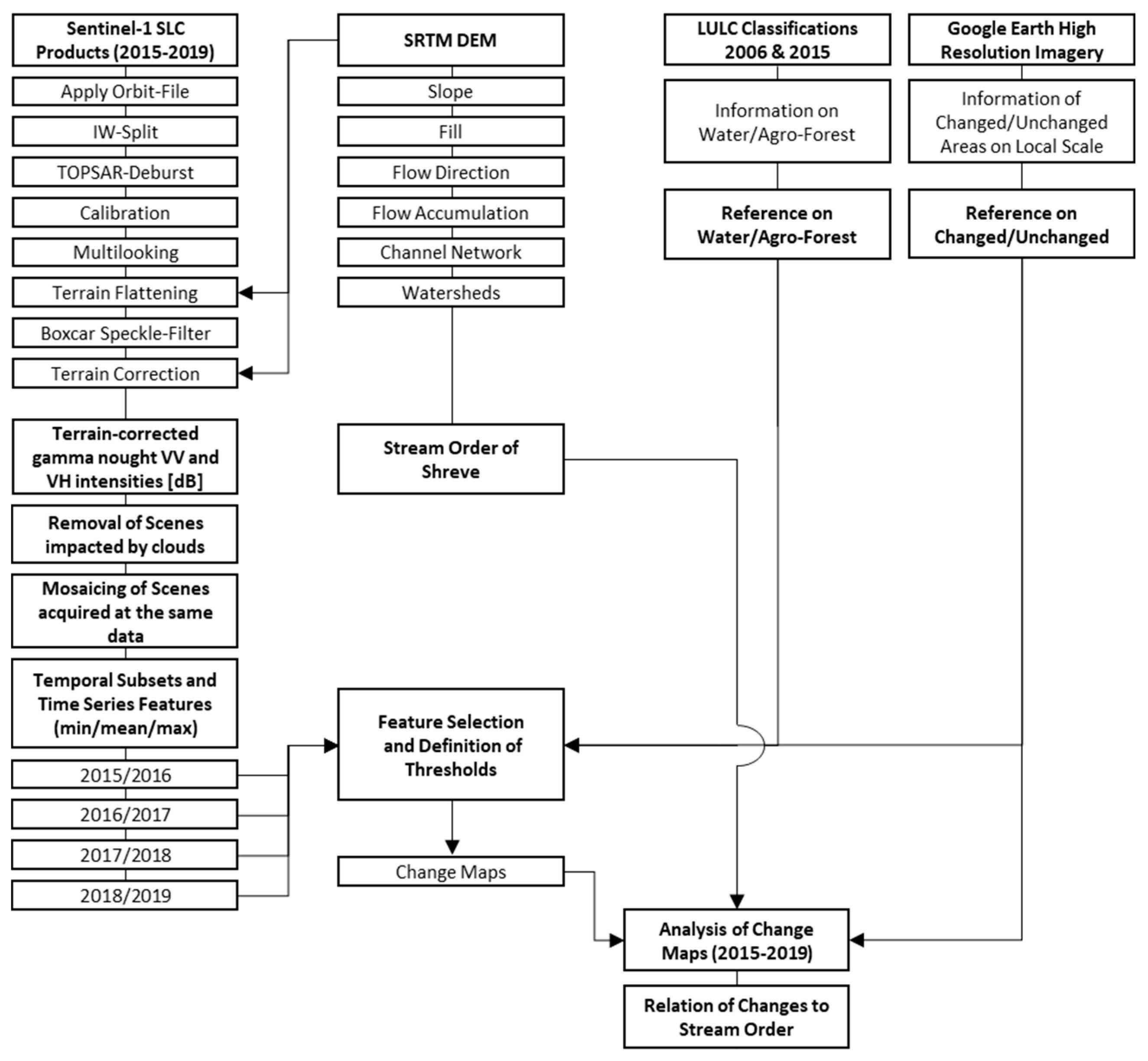
In this study, annual S-1 (Sentinel-1) time-series data from 2015 to 2019, together with reference data from Google Earth and existing land cover data, were analyzed using change detection techniques to map and monitor illegal mining activities on an annual basis in South-Western Ghana. The methodology was premised on the fact that mining-induced land cover changes can be detected based on changes in the scattering characteristics of time-series images acquired with the same acquisition geometry. The sensitivity of three time-series features (i.e., minimum, mean and maximum backscattering intensity observed within one year) to mining-induced changes (e.g., clearing of vegetation) was first conducted, after which analysis was performed to determine a threshold suitable to identify/classify changed and unchanged areas.

The use of time-series features proved useful for detecting inter-annual mining-induced changes along river bodies. Compared to the mean and maximum features, the minimum feature (in both VH and VV polarizations) performed better and was found to be more sensitive to changes in backscattering within the period investigated, including the lowest intensity values observed. A backscatter threshold value of +1.65 dB was found suitable to detect illegal mining activities in the study area. Application of the threshold revealed illegal mining area extents of 102 km², 60 km² and 33 km² for periods 2015/2016–2016/2017, 2016/2017–2017/2018 and 2017/2018–2018/2019, respectively. Our approach permitted the detection of new illegal mining activities on an annual basis, which revealed a decreasing trend in the period investigated. This is probably in response to government of Ghana’s efforts to sanitize the small-scale mining sector in the past couple of years.

Despite the advantages of Synthetic Aperture Radar data in monitoring phenomena in cloud-prone areas, our analysis revealed reasonable susceptibility of S-1 data to atmospheric conditions due to high intensity rainfall events. Scenes acquired in March and October, representing the beginning and ending of the rainy season, were the worst affected. A total of 29 out of 117 (ca. 25%) scenes could not be used in our analysis due to a strong local decrease in backscatter in the order >−10 dB compared to the long-term mean intensity and the undisturbed surroundings. This could have negatively affected our results considering the methodology employed. Further investigation of this finding in other geographies and climatic regions is required to ascertain the suitability of S-1 data for time-series dependent analysis such as the one employed in this study. Future studies can also benefit from an integration of Sentinel-2 data into the analysis.

The quantity and quality of the reference data was found to be a major challenge of this study. Google Earth Imagery permits a detailed view of changes in illegally mined areas. However, lack of sufficient images (spatially and temporarily) over the area analyzed due to excessive cloud cover limited the amount of reference data generated for this work. Future studies should consider embarking on an extensive field data collection to map changed and unchanged areas to serve as reference data.

References

1. Castello, L.; Macedo, M.N. Large-scale degradation of Amazonian freshwater ecosystems. Glob. Chang. Biol. 2016, 22, 990–1007. [Google Scholar] [CrossRef] [PubMed]
2. Kitula, A.G.N. The environmental and socio-economic impacts of mining on local livelihoods in Tanzania: A case study of Geita District. J. Clean. Prod. 2006, 14, 405–414. [Google Scholar] [CrossRef]
3. Sahu, H.; Dash, E. Land Degradation due to Mining in India and its Mitigation Measures. In Proceedings of the Second International Conference on Environmental Science and Technology, Singapore, Singapore, 26–28 February 2011; pp. 1–5. [Google Scholar]
4. Schueler, V.; Kuemmerle, T.; Schröder, H. Impacts of surface gold mining on land use systems in Western Ghana. Ambio 2011, 40, 528–539. [Google Scholar] [CrossRef] [PubMed] [Green Version]
5. Aryee, B.N.A. Ghana’s mining sector: Its contribution to the national economy. Resour. Policy 2001, 27, 61–75. [Google Scholar] [CrossRef]
6. Awudi, G.B.K. The role of foreign direct investment (FDI) in the mining sector of Ghana and the environment. In Proceedings of the Conference on Foreign Direct Investment and the Environment, OECD, Paris, France, 7–8 February 2002. [Google Scholar]
7. Hilson, G.; Hilson, A. Mining in Ghana Critical Reflections on a Turbulent Past and Uncertain Future; Oxford University Press: Oxford, UK, 2017. [Google Scholar]
8. Ghana Statistical Service. Gross Domestic Product; Ghana Statistical Service: Accra, Ghana, 2014. [Google Scholar]
9. ISSER. Overview: Global Economic Developments and Ghana’s Economic Performance. In The State of the Ghanaian Economy in 2014; University of Ghana: Institute of Statistical, Social, Economic Research: Accra, Ghana, 2015. [Google Scholar]
10. Afriyie, K.; Ganle, J.K.; Adomako, J.A.A. The good in evil: A discourse analysis of the galamsey industry in Ghana. Oxford Dev. Stud. 2016, 44, 493–508. [Google Scholar] [CrossRef]
11. Aragón, F.M.; Rud, J.P. Modern Industries, Pollution and Agricultural Productivity: Evidence from Mining in Ghana; Working Paper; International Growth Centre: London, UK, 2013. [Google Scholar]
12. Aragón, F.M.; Rud, J.P. Polluting industries and agricultural productivity: Evidence from mining in Ghana. Econ. J. 2015, 126, 1980–2011. [Google Scholar] [CrossRef]
13. Mantey, J.; Owusu-Nimo, F.; Nyarko, K.B.; Aubynn, A. Operational dynamics of “Galamsey” within eleven selected districts of western region of Ghana. J. Min. Environ. 2017, 8, 11–34. [Google Scholar] [CrossRef]
14. Dumett, R.E. El Dorado in West Africa: The Gold-Mining Frontier, African Labor, and Colonial Capitalism in the Gold Coast, 1875–1900; James Currey Publishers: Suffolk, UK, 1998. [Google Scholar]
15. Tsuma, W. Gold Mining in Ghana: Actors, Alliances and Power; LIT Verlag: Münster, Germany, 2010; Volume 15. [Google Scholar]
16. Crawford, G.; Botchwey, G. Conflict, collusion and corruption in small-scale gold mining in Ghana: Chinese miners and the state. Commonw. Comp. Politics 2017, 55. [Google Scholar] [CrossRef]
17. Graphic, D. New Policy Framework on Small-Scale Mining out on Friday. 2018. Available online: https://www.graphic.com.gh/news/general-news/ghana-news-govt-to-announce-new-policy-framework-on-small-scale-mining-friday.html (accessed on 26 March 2019).
18. JungleMiner. The Way Forward on the Ban of Small Scale Mining Activities in Ghana. 2018. Available online: https://jungleminer.com/the-way-forward-on-the-ban-of-small-scale-mining-activities-in-ghana/ (accessed on 26 March 2019).
19. Basommi, P.L.; Guan, Q.; Cheng, D. Exploring Land use and Land cover change in the mining areas of Wa East District, Ghana using Satellite Imagery. Open Geosci. 2015, 7, 618–626. [Google Scholar] [CrossRef]
20. Kusimi, J.M. Assessing land use and land cover change in the Wassa West District of Ghana using remote sensing. GeoJournal 2008, 71, 249–259. [Google Scholar] [CrossRef]
21. Snapir, B.; Simms, D.M.; Waine, T.W. Mapping the expansion of galamsey gold mines in the cocoa growing area of Ghana using optical remote sensing. Int. J. Appl. Earth Obs. Geoinf. 2017, 58, 225–233. [Google Scholar] [CrossRef] [Green Version]
22. Platnick, S.; King, M.D.; Ackerman, S.A.; Menzel, W.P.; Baum, B.A.; Riédi, J.C.; Frey, R.A. The MODIS cloud products: Algorithms and examples from Terra. IEEE Trans. Geosci. Remote Sens. 2003, 41, 459–473. [Google Scholar] [CrossRef] [Green Version]
23. Myjoyonline Galamsey War. Galamsey war IMCIM trains Pers. Oper. Synth. Aperture Radar Remote Sens. 2019. Available online: https://www.myjoyonline.com/news/2019/February-6th/galamsey-war-imcim-trains-personnel-on-operation-of-synthetic-aperture-radar-remote-sensing.php (accessed on 26 March 2019).
24. Almeida-Filho, R.; Shimabukuro, Y.E. Detecting areas disturbed by gold mining activities through JERS-1 SAR images, Roraima State, Brazilian Amazon. Int. J. Remote Sens. 2000, 21, 3357–3362. [Google Scholar] [CrossRef]
25. Telmer, K.; Stapper, D. Evaluating and Monitoring Small Scale Gold Mining and Mercury Use: Building a Knowledge-Base with Satellite Imagery and Field Work; University of Victoria: Victoria, BC, Canada, 2007. [Google Scholar]
26. Torres, R.; Snoeij, P.; Geudtner, D.; Bibby, D.; Davidson, M.; Attema, E.; Potin, P.; Rommen, B.; Floury, N.; Brown, M.; et al. GMES Sentinel-1 mission. Remote Sens. Environ. 2012, 120, 9–24. [Google Scholar] [CrossRef]
27. Attema, E. Mission Requirements Document for the European Radar Observatory Sentinel-1; European Space Agency: Paris, France, 2005; Volume 1. [Google Scholar]
28. Climate-Data.org. Climate Data for Cities Worldwide. Available online: https://en.climate-data.org/ (accessed on 15 June 2019).
29. Mudge, A.D.; Orozco, J.; Philips, T.K.; Antoine, P. The cetoniine fauna of the Upper Guinean forests and savannas of Ghana (Coleoptera: Scarabaeidae: Cetoniinae). Terr. Arthropod Rev. 2012, 5, 113–174. [Google Scholar] [CrossRef]
30. Tarboton, D.G.; Bras, R.L.; Rodriguez-Iturbe, I. On the extraction of channel networks from digital elevation data. Hydrol. Process. 1991, 5, 81–100. [Google Scholar] [CrossRef]
31. Gessner, U.; Machwitz, M.; Esch, T.; Tillack, A.; Naeimi, V.; Kuenzer, C.; Dech, S. Multi-sensor mapping of West African land cover using MODIS, ASAR and TanDEM-X/TerraSAR-X data. Remote Sens. Environ. 2015, 164, 282–297. [Google Scholar] [CrossRef]
32. El Hajj, M.; Baghdadi, N.; Zribi, M.; Angelliaume, S. Analysis of Sentinel-1 radiometric stability and quality for land surface applications. Remote Sens. 2016, 8, 406. [Google Scholar] [CrossRef] [Green Version]
33. Yang, J.; Qiu, X.; Ding, C.; Lei, B. Identification of stable backscattering features, suitable for maintaining absolute synthetic aperture radar (SAR) radiometric calibration of sentinel-1. Remote Sens. 2018, 10, 1010. [Google Scholar] [CrossRef] [Green Version]
34. Cha, S.-H. Comprehensive survey on distance/similarity measures between probability density functions. City 2007, 1, 1. [Google Scholar]
35. Kittler, J.; Illingworth, J. On threshold selection using clustering criteria. IEEE Trans. Syst. Man. Cybern. 1985, SMC-15, 652–655. [Google Scholar] [CrossRef]
36. Congalton, R.G.; Green, K. Assessing the Accuracy of Remotely Sensed Data. Principles and Practices, 2nd ed.; CRC Press Inc: London, UK, 2009. [Google Scholar]
37. Danklmayer, A.; Chandra, M. Precipitation induced signatures in SAR images. In Proceedings of the 3rd European Conference on Antennas and Propagation, Berlin, Germany, 23–27 March 2009; pp. 3433–3437. [Google Scholar]
38. Alpers, W.; Zhang, B.; Mouche, A.; Zeng, K.; Chan, P.W. Rain footprints on C-band synthetic aperture radar images of the ocean-Revisited. Remote Sens. Environ. 2016, 187, 169–185. [Google Scholar] [CrossRef]
39. Baidu, M.; Amekudzi, L.K.; Aryee, N.A.J.; Annor, T. Assessment of Long-Term Spatio-Temporal Rainfall Variability over Ghana using Wavelet Analysis. Climate 2017, 5, 30. [Google Scholar] [CrossRef] [Green Version]
40. Friesen, J. Spatio-Temporal Rainfall Patterns in Northern Ghana; Universität Bonn: Bonn, Germany, 2002. [Google Scholar]
41. Cloude, S. Polarisation: Applications in Remote Sensing; Oxford University Press: Oxford, NY, USA, 2014. [Google Scholar]
42. Richards, J.A. Remote Sensing with Imaging Radar, Signals and Communication Technology; Springer: Berlin/Heidelberg, Germany, 2009. [Google Scholar]
43. Gorelick, N.; Hancher, M.; Dixon, M.; Ilyushchenko, S.; Thau, D.; Moore, R. Google Earth Engine: Planetary-scale geospatial analysis for everyone. Remote Sens. Environ. 2017, 202, 18–27. [Google Scholar] [CrossRef]
44. Owusu-Nimo, F.; Mantey, J.; Nyarko, K.B.; Appiah-Effah, E.; Aubynn, A. Spatial distribution patterns of illegal artisanal small scale gold mining (Galamsey) operations in Ghana: A focus on the Western Region. Heliyon 2018, 4. [Google Scholar] [CrossRef] [Green Version]
45. Awotwi, A.; Anornu, G.K.; Quaye-Ballard, J.A.; Annor, T. Monitoring land use and land cover changes due to extensive gold mining, urban expansion, and agriculture in the Pra River Basin of Ghana, 1986–2025. Land Degrad. Dev. 2018, 29, 3331–3343. [Google Scholar] [CrossRef]
46. Obodai, J.; Adjei, K.A.; Odai, S.N.; Lumor, M. Land use/land cover dynamics using landsat data in a gold mining basin-the Ankobra, Ghana. Remote Sens. Appl. Soc. Environ. 2019, 13, 247–256. [Google Scholar] [CrossRef]
47. Armah-Attoh, D. Afro Barometer. Dispatch 175; CDD Ghana: Accra, Ghana, 2017; p. 6. [Google Scholar]
Figure 1. Study area and data coverage: (a) regional overview; (b) topographic setting and major cities/towns; (c) hydrographic setting and coverage of Sentinel-1 (2015–2019).
Remotesensing 12 00911 g001
Figure 2. Schematic workflow of the processing and analysis of Sentinel-1 time series, the Shuttle Radar Topographic Mission (SRTM) digital elevation model and the reference datasets.
Remotesensing 12 00911 g002
Figure 3. Reference Data from Google Earth: (a,b) Google Earth Imagery 2015 (© Maxar Technologies), (c,d) Google Earth Imagery 2017 (Image © CNES/Airbus & © Maxar Technologies) and (e,f) mapped changes (red polygons) between 2015 and 2017 related to mining activity.
Remotesensing 12 00911 g003
Figure 4. Examples of locally-restricted patches showing strong local decrease in backscatter intensity in the Sentinel-1 time series (2015–2019): (a) VV Intensity 2 March 2017, (b) VV Intensity 23 October 2018, (c) VV Intensity 8 February 2019; (df) Mean VV Intensity (2015–2019), (gi) intensity values along profiles AB, CD, and EF, and (j) locations (dashed polygons) where patches were detected within the study area (extent shown in green color, see Figure 1) for the full time series (2015–2019). Background map in (j) draws the slope of the SRTM Digital Elevation Model.
Remotesensing 12 00911 g004
Figure 5. Boxplots on the land cover classes “water” (blue) and “agro-forest” (green) for Sentinel-1 time series features minimum (MIN), maximum (MAX), mean (MEAN) and for both polarization channels (VV/VH). Time series features were processed for the temporal subset “2016/2017”. The reference samples were taken from existing LULC classifications.
Remotesensing 12 00911 g005
Figure 6. Frequency distributions of the classes “unchanged” (gray/black) and “changed” (orange/red) for the VV/VH intensity differences between the two temporal subsets “2015/2016” and “2016/2017”. Results are shown for the time series features minimum (MIN) (a,c) and mean (MEAN) (b,d). Information on “unchanged” and “changed” samples were taken from Google Earth Imagery (see Section 2.3 and Figure 3). Smoothing of the histograms was done by averaging the frequencies of five consecutive bins.
Remotesensing 12 00911 g006
Figure 7. Example of detected changes using the mean and minimum VV intensities of the sets “2015/2016” and “2016/2017”: (a) Google Earth Imagery 2015 (© Maxar Technologies), (b) Google Earth Imagery 2017 (Image © CNES/Airbus & © Maxar Technologies), (c) changes between 2015 and 2017 related to mining activity based on visual interpretation, (d) VV mean intensity “2015/2016”, (e) VV mean intensity “2016/2017”, (f) difference in VV mean intensities between sets “2015/2016” and “2016/2017” (d,e), (g) VV minimum intensity “2015/2016”, (h) VV minimum intensity “2016/2017” and (i) difference in VV minimum intensities between sets “2015/2016” and “2016/2017” (g,h).
Remotesensing 12 00911 g007
Figure 8. Classification of changes based on two different thresholds: (a) location of the subset within the study area, (b) difference in VH minimum intensities between sets “2015/2016” and “2016/2017”, (c) difference in VH minimum intensities between sets “2016/2017” and “2017/2018”, (d) difference in VH minimum intensities between sets “2017/2018” and “2018/2019”, (eg) classification using a threshold of +1.65 dB identified via the histogram intersection (see Table 2) and (hj) classification using a threshold of +2.78 dB identified via the Otsu Algorithm (see Table 2). Note: blue polylines show the channel network (see Section 2.2.2). A majority filter of 5 by 5 pixels was applied in the post-classification to classifications (ej) (Section 2.3.2).
Remotesensing 12 00911 g008
Figure 9. Classification of changes using VH polarization, the minimum intensity (time series feature) and the threshold from histogram intersection (+1.65 dB): (a) regional overview; (b) topographic and hydrographic setting (based on SRTM DEM), major cities and coverage of Sentinel-1 time series (2015–2019), (c) change map “2015/2016”–“2016/2017”, (d) change map “2016/2017”–“2017/2018” and (e) change map “2017/2018”–“2018/2019”.
Remotesensing 12 00911 g009
Figure 10. Classification of changes using VH polarization, the minimum intensity (time series feature) and the threshold from histogram intersection (+1.65 dB). Results displayed as change density (i.e., sum of changed pixels in a 1 km radius): (a) regional overview; (b) topographic and hydrographic setting (based on SRTM DEM), major cities and coverage of Sentinel-1 time series (2015–2019), (c) density change map “2015/2016”–“2016/2017”, (d) density change map “2016/2017”–“2017/2018” and (e) density change map “2017/2018”–“2018/2019”. Density was estimated by summing all changed pixels within a 1 km radius.
Remotesensing 12 00911 g010
Figure 11. Summary statistics on classifications shown in Figure 10: (a) total area identified as “changed” per period and (b) mean values of Average (Avg.), Minimum (Min.) and Maximum (Max.) Shreve Order per period. Shreve order values were deduced from the hydrographic analysis of the SRTM DEM. Changed areas and Shreve order were linked via a spatial join.
Remotesensing 12 00911 g011
Figure 12. Comparison of climate records and summary statistics of Sentinel-1 time series images affected by atmospheric effects (2015–2019): (a) monthly average temperature and precipitation at stations Prestea, Ayanfuri, and Obuasi (Source: climate-data.org) and (b) frequency of S-1 scenes showing a strong local decrease in the backscatter intensity due to clouds, shown as a percentage of all available scenes per month.
Remotesensing 12 00911 g012