Radiometric Comparison within the Sentinel-1 SAR Constellation over a Wide Backscatter Range

Abstract

Radiometric calibration adjusts the measured pixel intensity to a physical property, the radar cross section (RCS). After calibration, this relationship is defined over the entire backscatter range: from low image power (near noise) up to high reflections (below saturation). Based on a proper radiometric calibration, the measured radar backscatter for the Sentinel-1 synthetic aperture radar (SAR) satellite constellation is validated over a wide backscatter range using different target types. Therefore, the RCS derived from point targets and radar brightness from distributed targets are compared between Sentinel-1A (S-1A) and Sentinel-1B (S-1B) acquisitions over the same observation area for regions where a stable target backscatter is expected for a certain period of time. Low differences (in the order of 0.3 dB) are found between S-1A and S-1B for high and medium backscatter derived from point targets or rainforest regions, but higher differences for low backscattering regions like ice areas and lakes. For comparing radar brightness containing low backscatter targets, an accurate derived noise level has to be taken into account. In addition to the measured lower noise equivalent beta zero (NEBZ) level, higher transmit power was detected for S-1B compared to S-1A. The higher antenna gain of S-1B leads finally to a higher sensitivity for low backscattering areas of S-1B compared to S-1A and explains the found differences.

1. Introduction

One of the main reasons for building a space-borne radar constellation instead of operating a single instrument only is the higher revisit rate for acquisitions over the area of interest. For synthetic aperture radar (SAR), a number of such radar constellations are currently in operation [1], e.g., SAR-Lupe (5 satellites), COSMO-SkyMed [2,3] (4 satellites), or a synchronized operation of the TerraSAR-X/TanDEM-X formation [4] and the PAZ satellite [5]. The Radarsat constellation mission (3 satellites) was lunched recently in June 2019 [6]. Within virtual constellations [7] instruments from different platforms are combined; in particular, multi-temporal products can be derived by merging multiple SAR sources or even combining these with optical instruments [8]. However, SAR constellation missions using small satellites could reduce the mission costs dramatically. Such missions are planned for future developments [9] – related concepts are under investigation or within the development phase [10].

In the frame of the COPERNICUS program, the European Space Agency (ESA) was planned and realized a fleet of Sentinel-1 satellites [11]. The first one, Sentinel-1A (S-1A), is a single SAR satellite which was launched in April 2014. The SAR constellation was completed two years later after starting the operation of Sentinel-1B (S-1B). Both satellites carry a nearly identical payload: a C-band SAR operated at a center frequency of $5.405$ GHz and a maximum bandwidth of 100 MHz. The 280 transmit and receive modules (TRMs) of the phased array antenna are able to transmit a nominal peak power of about 5 kW. Both satellites S-1A and S-1B are flying a sun synchronized dusk-dawn orbit with an interferometric revisit time of twelve days each. By flying both satellites in the same orbit plane with 180${}^{\circ }$ orbital phasing difference, the revisit time is reduced to six days. Current observation scenarios for both satellites are available online: https://sentinel.esa.int/web/sentinel/missions/sentinel-1/observation-scenario. Continuing operation of this Sentinel-1 SAR constellation shall be ensured for the next decades: both satellites S-1A and S-1B will be replaced after their end of operation by S-1C and S-1D, respectively.

SAR instruments detect the elapsing time of transmitted pulses received at the instrument, as well as the measured backscatter power and phase information acquired from target objects. During SAR data processing, the measured raw data is focused and converted into a two dimensional image mapping the observation area. Radiometric calibration is necessary to allow a valid conversion of the observed pixel intensity into a physical relevant unit, e.g., radar cross section (RCS). Therefore, the whole SAR system has to be calibrated and various geometric and radiometric corrections have to be applied. The internal calibration compensates gain and phase variations of the instrument which may occur due to different temperatures and ensures the specified radiometric stability of the instrument over time. Furthermore, the knowledge of the antenna pointing is important to properly apply the antenna pattern correction during SAR data processing, which defines the relative radiometric accuracy within a SAR image. Absolute radiometric calibration has to be finally applied using reference targets on ground (e.g., corner reflectors and transponders) with well known RCS.

On behalf of ESA, the German Aerospace Center (DLR) performed independent calibration campaigns for both Sentinel-1s during their commissioning phases: for S-1A in 2014 [12] and for S-1B in 2016 [13]. Since then, both SAR instruments were permanently checked during routine operations [14] w.r.t. the radiometric accuracy and stability using corner reflectors and C-band transponders remotely controlled and deployed within the DLR calibration site [15].

Well calibrated SAR data products with accurately measured radar brightness are required for a number of applications and compose the basis for the quality of higher level products. The measured radar brightness can be exploited for various scientific applications and used to classify or even quantify the observed target area, e.g., ice areas [16], forests or other kinds of vegetation [17], soil moisture of wetland and grassland [18], as well as ocean currents or wind speeds [19]. By using a radar constellation it is important that each sensor produces comparable results, in particular in terms of measuring backscatters. In an ideal case, the same results should be achieved for the same observation area under constant conditions for each instrument so that the users do not have to care about the sensor used for acquiring the scene. This comparability should be valid over the whole backscattering range from targets with a very high signal-to-noise ratio (SNR) down to noise level.

The current study evaluates the intercomparability of S-1A and S-1B in terms of detected radar brightness and investigates reasons for found discrepancies. First, RCSs derived from point targets are evaluated and compared between S-1A and S-1B over a two-year observation period. Similar to SAR system calibration, the absolute radiometric accuracy and stability for both SAR instruments is derived from these measurements. These reference targets are appropriated for calibration purposes due to their high signal-to-clutter ratio and a negligible impact of system noise. Based on these results, the radar brightness of distributed targets are evaluated for different backscatter regimes: starting from medium backscatter found in Amazon rainforest areas over lower values in ice areas of Greenland down to near noise backscatters which are expected for calm water. For these different target types the radiometric stability and the comparability between S-1A and S-1B are analyzed.

For targets with low SNR (below about 10 dB), the impact of system noise is no more negligible and has to be taken into account. The accuracy of determined low radar brightness depends on the accuracy of the derived noise but is also limited by the noise level itself. Therefore, the noise level of S-1A and S-1B is also compared and the impact of noise on low backscatter is analyzed. Finally, the transmit power of both SAR instruments is compared by using transponder (ground receiver) recordings. The used data and methods are introduced in Section 2, the results are presented in Section 3 and discussed in Section 4, and Section 5 concludes the paper.

2. Materials and Methods

2.1. Sentinel-1 SAR Data Products

For the current study, SAR data products of S-1A and S-1B are used. The radar brightness ${\beta }^0$ is derived from the pixel intensity of calibrated level 1 slantrange complex (SLC) products using annotated look-up tables and the annotated calibration factor. These SAR data products are freely available, e.g., on the Copernicus open access hub (https://scihub.copernicus.eu).

Sentinel-1 can be operated in different modes – each offers a specific swath width and spatial resolution [20]. The highest resolution is given for the Stripmap mode with a resolution of 5 m by 5 m in azimuth and range and a swath width of about 80 km. The largest swath width of about 400 km is available for the extra-wide swath mode (EW) which provides a reduced geometric resolution of 20 m (range) by 40 m (azimuth). However, the main mode of Sentinel-1 is the interferometric wide-swath mode (IW) with a swath width of about 250 km and a medium geometric resolution of 5 m (range) by 20 m (azimuth). For the latter, in both modes the antenna is electronically steered within five and three subswathes for EW- and IW-mode, respectively. Dual-polarization products are available for Stripmap, EW-, and IW- mode; they offer co- and cross-pol images for a given transmit polarization H or V. The current study focuses on IW mode as the main mode using dual-polarization products (VV+VH or HH+HV).

2.2. Reference Targets

The Microwave and Radar Institute of the German Aerospace Center (DLR) has established a SAR calibration center for preparing and executing calibration of spaceborne SAR systems, like TerraSAR-X [21], TanDEM-X [22] or S-1A [12], and S-1B [13]. Part of this center is a calibration site consisting of six automatically operated reference targets: three trihedral corner reflectors and three C-band transponders [14]. These targets are remotely controlled and permanently monitored for their health status. Each target is aligned by schedule in the expected line-of-sight direction for an upcoming satellite overpass for both ascending and descending orbits. The corner reflectors have a leg length of 2.8 m which corresponds in C-band to a RCS of 49.2 dB m${}^2$. The high mechanical tolerance of 1 mm ensures an absolute radiometric accuracy for these targets of 0.2 dB (1$\sigma$). The C-band transponders have a center frequency of 5.405 GHz and a bandwidth higher than 100 MHz corresponding to the characteristics of the Sentinel-1 SAR instrument. The transponders are temperature controlled and automatically adjusted by their own internal calibration facility before each overpass to ensure a radiometric stability below 0.1 dB (1$\sigma$). An absolute radiometric accuracy of 0.2 dB (1$\sigma$) was achieved by executing and analyzing different calibration methods [23].

The transponders are also able to operate as ground receivers. Using this feature, the transmitted SAR antenna pattern can be recorded at ground in order to analyze the relative power of the SAR instrument and to derive the related azimuth antenna pointing [24]. Each transponder consists of two antennae: one to receive (RX) and one to retransmit (TX) the electromagnetic pulses. Both antennae are rotated by 45${}^{\circ }$ along the line-of-sight axis. This allows receiving both polarization signals (H and V) transmitted by the SAR instrument with the transponder but also receiving both signals (H and V) at the SAR instrument retransmitted by the transponder. This enables radiometric evaluation also for crosspolarized products (HV and VH). In contrast to this, trihedral corner reflectors show impulse responses for copolarized SAR images only (HH, VV) as the polarization of an incidence wave is not rotated by a trihedral corner reflector.

2.3. Deriving Radar Backscatter from Distributed and Point Targets

Point targets (like corner reflectors) usually produce a strong reflection which originates from a dominant scatterer within the observed resolution cell. In contrast, a distributed target consists of a large number of randomly distributed scatterers within a resolution cell. Each scatterer contributes with a random phase leading to variability in the magnitude even for the same target type in different resolution cells. Statistically, distributed targets like forests, grassland, or ice areas show specific mean radar backscattering coefficients which depend on observation parameters like radar wavelength, incidence angle, and target type [25].

The radar brightness ${\beta }^0$ of a SAR image pixel is calculated by the following formula [26,27]:

$${\beta }^0=\frac{{\left|D{N}_i\right|}^2}{A_{dn}^2·K}$$

(1)

$D{N}_i$ is the digital number of the complex image pixel at location i, $A_{dn}$ is the pixel scaling, and K is the absolute calibration factor. For estimating the radar brightness of a distributed target, all values regarding the target area are averaged in linear scale and then converted to logarithmic scale ${\beta }^0$ [dB] = 10 · log10(${\beta }^0$).

The noise level has to be considered for deriving a precise radar brightness, in particular for low backscattering targets with low SNRs. This is usually done by subtracting the mean noise floor ($P_{noise}$) from the observed backscatter data according to Equation (2). For the subtraction step, both values (image radar backscatter and scaled noise floor) have to be converted to linear scale; the result is then converted back to logarithmic scale afterwards.

$${\beta }_{noiseconsidered}^0=\frac{{\left|D{N}_i\right|}^2}{A_{dn}^2·K}-P_{noise}$$

(2)

For estimating the noise floor, usually specific noise pulses are applied. Nevertheless, deriving a precise and reasonable noise level is a challenging task which requires a deep knowledge about functionality and operating modes of the used SAR processor [28]. It should be noted that the noise floor is not constant over time and consists of several components of different origins including thermal receiver, background, quantization, and oscillator noise. Although the thermal noise is known to be the dominant component, the impact of background noise arising from the Earth surface is also not negligible. A noise floor difference of about 0.8 dB was derived for S-1B between different observation areas (sea and land) [29]. The Sentinel-1 noise floor is further investigated in a few publications by analyzing very low backscatter data [30,31]. In particular for the EW mode, it was shown that the originally derived noise level annotated within the SAR products was not estimated precisely enough by the former SAR processor version, especially for EW1. As a consequence, the noise estimation procedures were improved [32], leading to an updated version of the SAR processor in early 2019.

In order to estimate the absolute radiometric accuracy of a SAR system, the RCS values of reference targets are derived from SAR images and compared with the nominal RCS of these targets. This nominal RCS is either known from theory (e.g., for trihedral corner reflectors) or precisely derived from measurements (e.g., for transponders) [33,34]. The RCS of a point target is estimated from a SAR image by analyzing its impulse response function by taking into account the following subtasks:

• the impulse response is interpolated to a subpixel resolution,
• the integrated pixel method is used which considers the cumulated power related to the target response (see [35,36]),
• the background clutter is properly estimated and subtracted.

The RCS is finally estimated from the SAR image using the integrated image power $I_P$ of the impulse response multiplied with the pixel area $P_A$ and divided by the absolute calibration factor K [37].

$$RCS=\frac{I_P·P_A}{K}$$

(3)

3. Results

The following subsections present the results and show how accurate and stable S-1A and S-1B are in terms of measuring radiometric backscatterer. The comparison of the results between S-1A and S-1B with the same geometric conditions (e.g., elevation angle) shows the intercomparability between both SAR instruments. The different target types focus on different backscatter regimes covering point targets with high SNR but also distributed targets such as the Amazon rainforest with medium SNR, down to backscatter near noise found in ice areas and calm waters.

3.1. Point Target Evaluations

The differences between the observed RCS derived from SAR images and the theoretical expected RCS of the DLR reference targets are depicted in Figure 1 for S-1A (top) and S-1B (bottom) as a function of time. The trihedral corner reflectors produce impulse responses only for copolarized products. Thus results from the VV-polarization channel (red) containing both transponder and corner reflector RCS appear more often compared to VH-polarization channel (blue) which represents transponder results only. The RCS differences spread around 0 dB and indicate that both SAR instruments are well balanced in terms of radiometric calibration in general. However, both subfigures show small drifts over time (up- and down) in the order of 0.3 dB over several months. This behavior may arise from season related environment effects, e.g., due to more rainy days in summer compared to winter or remaining SAR instrument drifts.

The overall mean values and standard deviations for both SAR instruments and polarization channels related to the observation period are summarized in

Table 1. RCS deviations derived from reference point targets reported as mean values and standard deviations ($\mu$ ± $\sigma$) for both SAR instruments and polarization channels.

Polarization	S-1A RCS [dB]	S-1B RCS [dB]	S-1A/S-1B
Channel	($\mathit{\mu }\pm \mathit{\sigma }$)	($\mathit{\mu }\pm \mathit{\sigma }$)	Difference [dB]
VV	−0.19 dB ± 0.21 dB	−0.11 dB ± 0.17 dB	−0.08 dB
VH	−0.03 dB ± 0.33 dB	−0.24 dB ± 0.26 dB	0.21 dB

. These values document a slightly higher radiometric variation seen for the VH- compared to the VV-polarization channels and also a slightly higher variation of S-1A compared to S-1B. However, the mean values verify the radiometric calibration and indicate the intercomparability of both SAR instruments. In particular, for the VV-polarization channel the overall mean RCS deviation is below 0.2 dB for both SAR instruments with a mean difference below 0.1 dB between S-1A and S-1B for this polarization channel. The highest RCS bias is seen for VH-polarization channel of S-1B with -0.24 dB which leads to a mean difference between S-1A and S-1B of 0.21 dB for this polarization channel.

The absolute radiometric accuracy can be derived from these point target evaluations using the standard deviations from Table 1 and considering additional error contributions, i.e., the long-term stability of the instrument of 0.05 dB (1$\sigma$), and the reference target accuracy of 0.20 dB (1$\sigma$). For the IW mode and the two-year observation period, the absolute radiometric accuracy is obtained to be 0.346 dB (1$\sigma$) and 0.302 dB (1$\sigma$) for S-1A and S-1B, respectively. Note that the requirement in terms of absolute radiometric accuracy is 1 dB (3$\sigma$) for Sentinel-1; propagation effects are neglected.

The next step focuses on the acquisition geometry by grouping the derived RCS differences as a function of look angle. Therefore, the mean RCS deviation for each reference target is plotted for the given look angle in Figure 2 for S-1A (left) and S-1B (right). The results cover all three subswathes (IW1 – IW3) over a wide look angle range of about 12${}^{\circ }$ (from 27${}^{\circ }$ to 39${}^{\circ }$) which corresponds to an antenna elevation angle range from about −3${}^{\circ }$ to +9${}^{\circ }$ for this observation area. Each target is depicted by a specific symbol in Figure 2 and appears at different look angles related to three different satellite tracks used. As before, VV-polarization results (red symbols) are available for both target types (corner reflectors and transponders), while the RCS deviation for VH-polarization channels (blue) can be derived for transponders only.

A radiometric variation over look angle is visible for S-1A compared to S-1B within Figure 2. Furthermore, the spatial variation over look angle is even slightly higher compared to the temporal variation expressed by the standard deviation (error bar) for each target at a constant elevation angle which is below 0.15 dB. In particular, for the cross-polarization channel, the mean values differ up to 0.5 dB at different look angles even for the same reference target. Such radiometric variations over the elevation angle may arise from remaining uncertainties of the antenna pattern compensation executed during SAR data processing, as already analyzed [12,13,14].

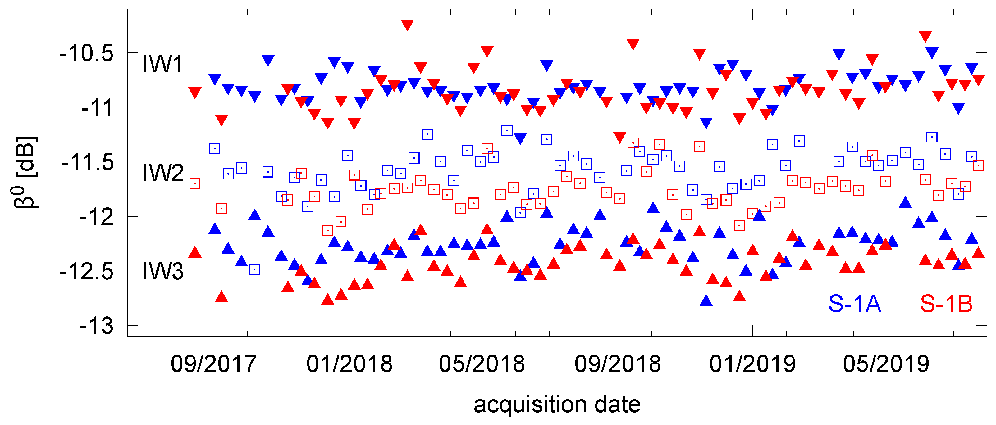
3.2. Medium Radar Backscatter Areas (Amazon Rainforest)

In order to further validate the radiometric comparability between both SAR instruments, the radar brightness ${\beta }^0$ is derived from distributed targets from areas within the Amazon rainforest with medium radar backscatterer and a sufficient SNR above 15 dB for copolarized and above 10 dB for cross-polarized channels. For this purpose, three regions are defined with a pixel size of 1000 by 700 pixels (range, azimuth) representing vignettes of about 23 km${}^2$ in slantrange geometry. These distributed targets are spread over all three IW subswathes (Figure 3) and compose a wide coverage w.r.t. antenna elevation from near to far range. By visual inspection, these vignettes are found to contain mainly homogeneous forest areas without disturbing orographic features like rivers or deforested areas. Note that as radar brightness depends on the local incidence angle, slightly different average values are expected for each observation area.

The derived radar brightness for the different observation areas are evaluated as a function of acquisition time over a two year observation period. Within Figure 4 the HV channel results are depicted for both SAR instruments: S-1A (blue) and S-1B (red). The related mean values and standard deviations for co- and cross-polarized channels are summarized in

Table 2. Mean radar brightness and standard deviations ($\mu$ ± $\sigma$) from three different observation areas within the Amazon rainforest.

Target Center [lat,lon]	pol	S-1A ${\mathit{\beta }}^0$ [dB]	S-1B ${\mathit{\beta }}^0$[dB]	S-1A/S-1B
@ Subswath		($\mathit{\mu }\pm \mathit{\sigma }$)	($\mathit{\mu }\pm \mathit{\sigma }$)	Difference [dB]
7.18${}^{\circ }$ S, 66.61${}^{\circ }$W	HH	−4.75 ± 0.18	−4.92 ± 0.20	0.17
IW1	HV	−10.81 ± 0.15	−10.86 ± 0.21	0.05
7.08${}^{\circ }$ S, 65.76${}^{\circ }$W	HH	−5.54 ± 0.21	−5.87 ± 0.19	0.33
IW2	HV	−11.57 ± 0.21	−11.75 ± 0.17	0.18
6.85${}^{\circ }$ S, 65.02${}^{\circ }$W	HH	−6.29 ± 0.19	−6.73 ± 0.15	0.44
IW3	HV	−12.25 ± 0.18	−12.43 ± 0.32	0.18

. The radar backscatter decreases from near range (IW1) to far range (IW3) due to the corresponding local incidence angle of the observed area. The radar brightness of each zone shows only slight variations and trends over time (Figure 4) which are expressed by standard deviations in the order of 0.2 dB (Table 2). Low differences are found between S-1A and S-1B; the ratios between the averaged radar brightness are low between 0.05 dB and 0.44 dB.

3.3. Transition to Lower Backscatterer (Greenland Region)

In order to further investigate the radiometric intercomparability of both instruments for lower backscatterer, distributed targets with stable SNRs are sought which can be used for long-term evaluations covering a sufficient backscattering range. For this purpose ice areas within the Greenland region are chosen which cover a wide range of related radar brightness. These values are strongly dependent on the incidence angle and reach values between −12 dB and −5 dB for the copolarized channels and between −22 dB and −15 dB for the cross-polarized channels. Five different distributed targets are defined by selecting observation areas of 1000 by 700 pixels (range, azimuth) covering all three IW subswathes with vignettes of about 23 km${}^2$ in slantrange geometry (Figure 5).

The radar brightness ${\beta }^0$ is calculated for each target from related SAR images using co- and cross-polarized channels. The HV polarization results for both S-1A and S-1B are depicted as a function of observation time within Figure 6; the mean values and standard deviations as well as the differences between S-1A and S-1B are summarized in

Table 3. Mean radar brightness and standard deviations ($\mu$ ± $\sigma$) of five selected areas within the Greenland ice region using HV polarization channel.

Observation	Sub	S-1A ${\mathit{\beta }}^0$ [dB]	S-1B ${\mathit{\beta }}^0$ [dB]	S-1A/S-1B
Area Center	Swath	($\mathit{\mu }\pm \mathit{\sigma }$)	($\mathit{\mu }\pm \mathit{\sigma }$)	Difference [dB]
A:  72.62${}^{\circ }$N, 33.70${}^{\circ }$W	IW1	−15.09 ± 0.05	−15.12 ± 0.11	0.03
B:  72.68${}^{\circ }$N, 34.40${}^{\circ }$W	IW1	−16.12 ± 0.06	−16.32 ± 0.09	0.20
C:  72.83${}^{\circ }$N, 34.92${}^{\circ }$W	IW2	−18.29 ± 0.13	−18.90 ± 0.15	0.61
D:  72.88${}^{\circ }$N, 35.68${}^{\circ }$W	IW2	−20.77 ± 0.11	−21.12 ± 0.10	0.35
E:  73.01${}^{\circ }$N, 38.32${}^{\circ }$W	IW3	−21.32 ± 0.05	−21.72 ± 0.10	0.40

.

As documented in Figure 6 and Table 3, the selected ice areas show a very low backscatter variation for the HV polarization channel over time; the highest standard deviation found is 0.13 dB. These values are in particular lower compared to the rainforest or Lake Constance observation area (shown in the next subsection). The differences between S-1A and S-1B measurements are between 0.03 dB and 0.61 dB.

3.4. Very Low Radar Backscatter (Calm Water Region at Lake Constance)

A distributed target with a very low radar backscatter and a low SNR can be found, e.g., within calm waters. For the study, a region of 1000 by 700 pixels (range, azimuth) located at Lake Constance (centered at 47.55${}^{\circ }$N, 9.49${}^{\circ }$E) is selected which is covered by subswath IW1 (Figure 7).

The averaged radar brightness for this area is evaluated and the VH channel results are depicted as a timeline in Figure 8 for S-1A (blue) and S-1B (red). Outliers may exit due to bad weather conditions or strong winds which have an impact on the water surface disturbing the calm water conditions and leading to significant higher backscatter power for these acquisitions. Therefore, results with radar brightness higher than 1 dB compared to the mean value are marked with open symbols and are not considered for the calculations of mean values and standard deviations.

Although the same observation area is evaluated for both SAR instruments, the average radar brightness differs between S-1A (−20.12 dB) and S-1B (−21.27 dB). The significant higher difference of 1.15 dB (compared to ∼0.2 dB found for the Amazon rainforest) for targets with low SNR seems to be related to the different noise levels for S-1A and S-1B for these acquisitions as discussed in the next section. The noise level is annotated in the related SAR product. The noise product quality is significantly improved since SAR processor version 2.90 [32] which has been operationally available since summer 2018. For the selected observation area, an average noise level of −20.87 dB for S-1A and −22.12 dB for S-1B are extracted from the SAR annotation products. The evaluated backscatter and noise values are summarized in

Table 4. Mean radar brightness and standard deviations ($\mu$ ± $\sigma$) of the low backscatter areas within Lake Constance (47.55${}^{\circ }$N, 9.49${}^{\circ }$E).

	S-1A	S1A	S-1B	S1B	S-1A/S-1B [dB]	S-1A/S-1B [dB]
Subswath	${\mathit{\beta }}^0$ [dB]	Noise	${\mathit{\beta }}^0$ [dB]	Noise	Noise not	Noise
	($\mathit{\mu }\pm \mathit{\sigma }$)	[dB]	($\mathit{\mu }\pm \mathit{\sigma }$)	[dB]	Subtracted	Subtracted
IW1-VH	−20.12 ± 0.18	−20.87	−21.27 ± 0.25	−22.12	1.15	0.65

. The radiometric stability over time is expressed by the standard deviations with 0.18 dB for S-1A and 0.25 dB for S-1B. These values are similar to the ones found for the Amazon rainforest.

3.5. Sensitivity of Noise Subtraction for Targets with Low SNR

In order to also derive an accurate radar brightness for targets with low SNR, the noise level has to be considered. Therefore, the noise power is subtracted from observed radar brightness in linear scale, i.e., both values (radar brightness and annotated noise) have to be converted to linear scale before the subtraction step. The noise subtracted backscatter as the result can be converted back to logarithmic scale afterwards. By subtracting the noise in that way, the resulting difference between S-1A and S-1B is reduced from 1.15 dB (without noise subtraction) to 0.65 dB (with noise subtraction) for the given observation area at Lake Constance (see Table 4).

For low SNR the noise subtraction is a necessary step for comparing two systems with different noise levels. For low SNR, the image power is only slightly higher than the noise power and the (linear) difference between both values is very small resulting in very low decibel values after reconverting to logarithmic scale. Hence, for areas with low SNR, the resulting noise subtracted backscatter difference between both SAR systems is very sensitive to the derived radar brightness and the estimated noise level. For the given case, the noise level of S-1A is higher than the noise of S-1B or even the measured radar brightness by S-1B. That indicates that S-1A has a higher system noise compared to S-1B (see Table 4). Consequently, S-1B is more sensitive to low backscatter compared to S-1A. Nevertheless, the same target area is observed under the same acquisition geometry and consequently this should result in a nearly equivalent noise subtracted backscatter value. One of the reasons for the remaining difference of 0.65 dB may be a not accurately enough estimated noise level.

The following case study evaluates the impact of noise accuracy on the resulting noise subtracted backscatter differences for low SNR from SAR observations of Lake Constance. The measured average image backscatter values of −20.12 dB for S1-A and −21.27 dB for S-1B (see Table 4) are used as fixed parameters – the effect from different noise levels is evaluated and depicted within Figure 9. For a SNR of 0 dB, the measured backscatter values are at noise level, marked by the arrow in the top right corner of the plot. In this case the noise subtracted backscatter is 0 at linear scale for both instruments, i.e., both instruments have different noise levels but are perfectly balanced. The black line marks the balanced case over the noise level range. For each point at the black line, the corresponding noise levels can be assigned to S-1A and S-1B. The noise subtracted image backscatter is well balanced between S-1A and S-1B for these noise pairs. The colored lines within Figure 9 indicate remaining imbalances of 0.5 dB, 1.0 dB, 1.5 dB, or 2.0 dB for the corresponding noise levels.

The annotated noise levels extracted from the related SAR products (see Table 4) are marked as a circle within Figure 9. The resulting difference of 0.65 dB between both noise subtracted backscatter values (see Table 4) is also expressed within the figure: the circle is located between green (0.5 dB) and blue line (1.0 dB) but near the green line. The error bars reflect the sensitivity of the ${\beta }^0$ difference between S1A and S1B in terms of noise variation. A hypothetical noise shift of 0.1 dB almost vanishes the ${\beta }^0$ difference in this case if S-1A noise increases or S-1B noise decreases. In this case the black line is almost reached. In the opposite case the discrepancy rises up to about 1.2 dB. The high noise dependency on the S1A/S1B difference is only visible for low SNR. If higher SNRs or lower absolute noise values are considered, the circle will move towards the lower left corner of the figure. In this region the colored lines are more separated from each other, i.e., a noise variation has a much lower impact on the resulting S1A/S1B difference. However, for comparing noise subtracted backscatter for low SNR, the noise estimation has to be very accurate. In the presented case, an error within the noise estimation of 0.1 dB explains a difference of noise subtracted backscatter between S-1A and S-1B of 0.65 dB.

4. Discussion

The discussion section summarizes the radiometric results derived from different target types w.r.t. their long-term radiometric stability and intercomparability between S-1A and S-1B over a wide backscatter range. By focusing on noise measurements and transponder recordings, the reasons for the different results derived from S-1A and S-1B in particular for low backscatter targets are further investigated and discussed.

4.1. Long-Term Radiometric Stability

In order to analyze the radiometric stability of the SAR instrument, the variation of radar backscatter for the different target types is investigated. The comparison of the derived standard deviation for the different target types and polarization channels is depicted by Figure 10 showing S-1A (blue) and S-1B (red) results. For this plot the same time range from Aug 2018 to Aug 2019 is selected for all target types. Furthermore, the backscatter results are grouped by the given acquisition geometry for each target, i.e., each standard deviation shown corresponds to a certain antenna elevation angle.

As visible in Figure 10, the derived standard deviation depends on the target type. As expected, the lowest standard deviations (below 0.15 dB) are found for the reference targets (corner reflectors and transponders) for co- and cross-polarized channel. The standard deviation derived for the ice areas are also very low; in particular for the cross-polarized channel the target stability is comparable to the artificial point targets. The rainforest regions and also the observed lake areas show a slightly higher backscatter variation but below 0.3 dB. Furthermore, the standard deviation in Figure 10, a measure for the observed stability, is nearly identical for both SAR instruments S-1A and S-1B. As the backscatter variation consists of contributions from both the observed targets and the SAR instrument, it is valid to use most stable targets for estimating the instrument stability. Thus, by focusing on stable targets (point targets and ice area) a radiometric stability of 0.1 dB can be verified for both SAR systems.

4.2. Radiometric Comparability between S-1A and S-1B over a Wide Backscatter Range

Summarizing all target types and polarization channels used to cover a wide backscatter range, the radiometric comparability between S-1A and S-1B is investigated by a direct backscatter comparison between both SAR instruments. Figure 11 depicts the radar backscatter difference as a function of SNR for distributed targets used. The lake results (dark blue) have the lowest SNR at about 0.8 dB, the ice area (blue) observed with cross-polarization channel shows low SNR below 10 dB; for the ice area with copolarized channel and the rainforest targets (green), medium SNR between 10 dB and 20 dB are visible.

In addition to distributed targets, results derived from point targets (black plus and cross signs) are also depicted for the differences between S-1A and S-1B within Figure 11. Due to the high RCS of the point targets, the related SNRs are significantly higher compared to the distributed targets. Therefore, the point target results are plotted at the right side of the graph. For point targets a low difference between the RCS derived from S-1A and S-1B is found: between −0.3 dB and +0.1 dB for the VV channel (plus symbols) and between +0.1 dB and +0.5 dB for the VH channel (cross symbols).

The radiometric intercomparability between S-1A and S-1B is expressed by the radar brightness differences for distributed targets and RCS differences for point targets as depicted in Figure 11. In addition to the observed image backscatter differences (full symbols), the noise subtracted backscatter differences (open symbols) are also plotted. For low SNRs (below about 10 dB) the noise impact is no more negligible; therefore, the noise should be subtracted for estimating and comparing radar brightness values. In all analyzed cases the noise subtraction improves the ${\beta }^0$ differences between S-1A and S-1B. Except for the lake case, the differences are between −0.3 dB and +0.5 dB and in a good agreement with the point target results. Note that for very low SNR values noise subtracted backscatter results are very sensitive to the noise and image power derived from the data.

4.3. Noise Data Analysis from Calm Ocean Acquisitions

As stated in the previous section, noise estimation has a high impact on the radiometric accuracy in particular for backscatter with low SNR. In order to analyze this impact, the noise level of S-1A and S-1B is directly compared. Therefore, radar acquisitions are used covering a wide area of very calm waters. These areas can be found in particular within the ocean near islands. For the current study, an observation area located in the Pacific ocean south of the Hawaiian islands is chosen where dual-polarized radar data are available for S-1A and S-1B. In particular for the cross-polarization channel it is expected that most parts of the transmitted energy are reflected by the smooth surface away from the incidence direction so that the instrument receives almost no backscatter energy from the surface and the SAR receiving channel contains mainly the instrument noise.

The radar brightness of the calm ocean region detected by the cross-polar channel is depicted in Figure 12 for two single IW mode acquisitions (S-1A and S-1B) with a six days time delay between S-1A and S-1B. In addition to the measured backscatter, the annotated noise levels are also plotted. In an ideal case, the annotated noise profiles should match the measured radar brightness as the received power in the cross-polar channel is expected to be instrument noise only. Note that instead of a constant noise level, the shape of the inverted two-way elevation antenna pattern is reflected within the figure as expected because these patterns have to be subtracted during SAR data processing accordingly. Such observations were already evaluated in order to derive the noise equivalent sigma zero (NESZ) of the Sentinel-1 SAR instrument [40].

The results within Figure 12 show that the annotated noise from S-1A nearly predicts basically the measured radar brightness ${\beta }^0$. Only for some regions (e.g., between 29${}^{\circ }$ and 30${}^{\circ }$ look angle within IW1) the measured ${\beta }^0$ is even lower than the predicted noise, i.e., the noise level may be slightly overestimated for these sections. For S-1B the measured backscatter is always higher compared to the annotated noise over the entire look angle range. This indicates that the noise level is not reached for S-1B within the selected calm ocean regions.

Furthermore, Figure 12 shows that the lowest detectable radar brightness (which is equivalent to the NEBZ) differs significantly between both SAR instruments by about 1.4 dB on average. S-1B can detect a lower backscatter level than S-1A or in other words, S-1B is more sensitive than S-1A. In addition to a lower noise level, the higher sensitivity may also arise from a higher two-way antenna gain due to a higher transmit power or a higher pattern gain for the transmit or the receive path or both. From the calm ocean measurements alone it is not decidable if the different sensitivity levels are due to different system noise, transmit power levels, or pattern gains of both SAR instruments.

4.4. Comparing the SAR Transmit Antenna Pattern Using Transponder Recordings

To further investigate the different sensitivity levels of both SAR instruments, transponder recordings were investigated. The DLR transponders are able to detect and record the transmitted signals of the SAR instrument during an overpass. These recordings are usually used to verify the antenna pointing and the transmit patterns in azimuth direction [24].

The maximum level of the transmit azimuth pattern measured by each transponder is estimated. For each transponder these gain values are averaged over at least 10 overpasses for a given constellation, i.e., same look angle and same internal transponder settings. These averaged gain values are shown as data points in Figure 13 for S-1A (blue points) and S-1B (red points), whereby the free space losses were already considered. For each setting a low standard deviation (below 0.2 dB) is found.

In order to compare the measurements with the theoretical expected gain shape, the SAR transmit elevation pattern derived from the Sentinel-1 antenna model is plotted as a function of look angle in Figure 13 (lines). The measured gain values match well the shape of the theoretical transmit elevation pattern. For all three transponders and all three geometric configurations used, a higher transmit pattern gain is found for S-1B compared to S-1A of about 0.7 dB on average.

It is concluded that the higher sensitivity of S-1B compared to S-1A arises on the one hand from a higher transmit power of about 0.7 dB. However, to explain the difference of about 1.4 dB between the NEBZ levels of both SAR instruments (see Figure 12) the remaining gain of 0.7 dB has to be related to a higher receive pattern gain of S-1B. The found reciprocity of transmit and receive pattern gain may indicate that the higher sensitivity of the S-1B SAR instrument arises mainly from the antenna radiation elements themselves.

5. Conclusions

The radiometric performance of S-1A and S-1B was evaluated for different target types covering a wide backscatter range from point targets with a high SNR to distributed targets like rainforest, ice area, and calm waters with medium or low SNR values. Using the known RCS of the DLR point targets (corner reflectors and transponders), an absolute radiometric accuracy of 0.346 dB (1$\sigma$) for S-1A and of 0.302 dB (1$\sigma$) for S-1B was derived for the IW mode covering a two-year observation period. The long-term radiometric stability of both instruments was verified to be in the order of 0.1 dB by focusing on the backscatter variations of targets observed with a given acquisition geometry, i.e., with a (nearly) constant SAR antenna elevation angle. Besides point targets, ice areas were also found to be stable targets over time. The backscatter intercomparability was analyzed by a direct comparison between S-1A and S-1B for the same targets observed by the same acquisition geometry. For point targets only small differences remain between S-1A and S-1B of −0.08 dB and 0.21 dB for the VV and VH polarization channel, respectively. Similar values were found for distributed targets with a medium SNR above 10 dB (rainforest and ice areas).

Furthermore, low backscatter targets with a SNR below 10 dB were analyzed by focusing on cross-polarized acquisitions of ice areas and calm waters. For these targets higher backscatter differences between S-1A and S-1B were found; e.g., up to 0.6 dB for the ice area and 1.1 dB for Lake Constance. The recommended noise subtraction step reduces these differences; nevertheless, remaining discrepancies are observed after noise subtraction in the order of 0.6 dB. The reason is that the accuracy of these noise subtracted backscatter signals is strongly dependent on the quality of the estimated noise levels. It was shown that in case of low SNR (e.g., 0.8 dB) a backscatter difference of 0.6 dB may arise from an inaccuracy of the estimated noise level in the order of only 0.1 dB.

However, it was shown that for low SNR targets, S-1B shows systematically lower radar brightness compared to S-1A – in the extreme case, the observed NEBZ acquired for cross-polarized channels over calm waters differs by about 1.4 dB. From this fact it was concluded that S-1B is more sensitive compared to S-1A. From evaluations of transponder recordings, a higher transmit pattern gain of about 0.7 dB was observed for S-1B compared to S-1A. Taking furthermore the reciprocity of the passive radiation antenna elements into account, the receive pattern gain of S-1B must also be higher compared to S-1A by about 0.7 dB, yielding the highest observed backscatter difference of 1.4 dB over calm waters.

References

1. Sandau, R.; Brieß, K.; D’Errico, M. Small satellites for global coverage: Potential and limits. ISPRS J. Photogramm. Remote Sens. 2010, 65, 492–504. [Google Scholar] [CrossRef]
2. Milillo, P.; Riel, B.; Minchew, B.; Yun, S.; Simons, M.; Lundgren, P. On the Synergistic Use of SAR Constellations’ Data Exploitation for Earth Science and Natural Hazard Response. IEEE J. Sel. Top. Appl. Earth Observ. Remote Sens. 2016, 9, 1095–1100. [Google Scholar] [CrossRef]
3. Battagliere, M.L.; Virelli, M.; Lenti, F.; Lauretta, D.; Coletta, A. A Review of the Exploitation of the Operational Mission COSMO-SkyMed: Global Trends (2014-2017). Space Policy 2019, 48, 60–67. [Google Scholar] [CrossRef]
4. Buckreuss, S.; Schättler, B.; Fritz, T.; Mittermayer, J.; Kahle, R.; Maurer, E.; Böer, J.; Bachmann, M.; Mrowka, F.; Schwarz, E.; et al. Ten Years of TerraSAR-X Operations. Remote Sens. 2018, 10, 873. [Google Scholar] [CrossRef] [Green Version]
5. Gantert, S.; Kern, A.; Düring, R.; Janoth, J.; Petersen, L.; Herrmann, J. The future of X-band SAR: TerraSAR-X next generation and WorldSAR constellation. In Proceedings of the 2013 Asia-Pacific Conference on Synthetic Aperture Radar (APSAR), Tsukuba, Japan, 23–27 September 2013; pp. 20–23. [Google Scholar]
6. CSA News, published on 12th June 2019. Available online: https://www.canada.ca/en/space-agency/news/2019/06/canadas-next-generation-radarsat-satellite-constellation-successfully-launches-to-space.html (accessed on 6 March 2020).
7. Wulder, M.A.; Hilker, T.; White, J.C.; Coops, N.C.; Masek, J.G.; Pflugmacher, D.; Crevier, Y. Virtual constellations for global terrestrial monitoring. Remote Sens. Environ. 2015, 170, 62–76. [Google Scholar] [CrossRef] [Green Version]
8. Callegari, M.; Marin, C.; Notarnicola, C. Multi-temporal and multi-source alpine glacier cover classification. In Proceedings of the 2017 9th International Workshop on the Analysis of Multitemporal Remote Sensing Images (MultiTemp), Brugge, Belgium, 27–29 June 2017; pp. 1–3. [Google Scholar] [CrossRef]
9. Krieger, G.; Moreira, A. Multistatic sar satellite formations: potentials and challenges. In Proceedings of the 2005 IEEE International Geoscience and Remote Sensing Symposium, Seoul, Korea, 25–29 July 2005; Volume 4, pp. 2680–2684. [Google Scholar]
10. Farquharson, G.; Woods, W.; Stringham, C.; Sankarambadi, N.; Riggi, L. The Capella Synthetic Aperture Radar Constellation. In Proceedings of the EUSAR 2018 12th European Conference on Synthetic Aperture Radar, Aachen, Germany, 4–7 June 2018. [Google Scholar]
11. Torres, R.; Snoeij, P.; Geudtner, D.; Bibby, D.; Davidson, M.; Attema, E.; Potin, P.; Rommen, B.; Floury, N.; Brown, M.; et al. GMES Sentinel-1 mission. Remote Sens. Environ. 2012, 120, 9–24. [Google Scholar] [CrossRef]
12. Schwerdt, M.; Schmidt, K.; Tous Ramon, N.; Castellanos Alfonzo, G.; Döring, B.; Zink, M.; Prats, P. Independent Verification of the Sentinel-1A System Calibration. IEEE J. Sel. Top. Appl. Earth Observ. Remote Sens. 2016, 9, 994–1007. [Google Scholar] [CrossRef] [Green Version]
13. Schwerdt, M.; Schmidt, K.; Ramon, N.T.; Klenk, P.; Yague-Martinez, N.; Prats-Iraola, P.; Zink, M.; Geudtner, D. Independent System Calibration of Sentinel-1B. Remote Sens. 2017, 9, 511. [Google Scholar] [CrossRef] [Green Version]
14. Schmidt, K.; Tous Ramon, N.; Schwerdt, M. Radiometric Accuracy and Stability of Sentinel-1A Determined using Point Targets. Int. J. Microw. Wirel. Technol. 2018, 10, 538–546. [Google Scholar] [CrossRef] [Green Version]
15. Reimann, J.; Schwerdt, M.; Schmidt, K.; Ramon, N.T.; Döring, B. The DLR Spaceborne SAR Calibration Center. Frequenz 2017, 71, 619–627. [Google Scholar] [CrossRef]
16. Nagler, T.; Rott, H.; Hetzenecker, M.; Wuite, J.; Potin, P. The Sentinel-1 Mission: New Opportunities for Ice Sheet Observations. Remote Sens. 2015, 7, 9371–9389. [Google Scholar] [CrossRef] [Green Version]
17. Garestier, F.; Dubois-Fernandez, P.C.; Papathanassiou, K.P. Pine Forest Height Inversion Using Single-Pass X-Band PolInSAR Data. IEEE Trans. Geosci. Remote Sens. 2008, 46, 59–68. [Google Scholar] [CrossRef]
18. Gao, Q.; Zribi, M.; Escorihuela, M.J.; Baghdadi, N. Synergetic Use of Sentinel-1 and Sentinel-2 Data for Soil Moisture Mapping at 100 m Resolution. Sensors 2017, 17, 1966. [Google Scholar] [CrossRef] [PubMed] [Green Version]
19. Mouche, A.A.; Chapron, B.; Zhang, B.; Husson, R. Combined Co- and Cross-Polarized SAR Measurements Under Extreme Wind Conditions. IEEE Trans. Geosci. Remote Sens. 2017, 55, 6746–6755. [Google Scholar] [CrossRef]
20. Geudtner, D.; Torres, R.; Snoeij, P.; Davidson, M.; Rommen, B. Sentinel-1 system capabilities and applications. In Proceedings of the 2014 IEEE International Geoscience and Remote Sensing Symposium (IGARSS), Quebec City, QC, Canada, 13–18 July 2014; pp. 1457–1460. [Google Scholar]
21. Schwerdt, M.; Brautigam, B.; Bachmann, M.; Döring, B.; Schrank, D.; Gonzalez, J.H. Final TerraSAR-X Calibration Results Based on Novel Efficient Methods. IEEE Trans. Geosci. Remote Sens. 2010, 48, 677–689. [Google Scholar] [CrossRef]
22. Schwerdt, M.; Gonzalez, J.H.; Bachmann, M.; Schrank, D.; Schulz, C.; Döring, B. Monostatic calibration of both TanDEM-X satellites. In Proceedings of the 2010 IEEE International Geoscience and Remote Sensing Symposium, Honolulu, HI, USA, 25–30 July 2010; pp. 2636–2639. [Google Scholar]
23. Rudolf, D.; Raab, S.; Döring, B.J.; Jirousek, M.; Reimann, J.; Schwerdt, M. Absolute radiometric calibration of the novel DLR “Kalibri” transponder. In Proceedings of the 2015 German Microwave Conference, Nuremberg, Germany, 16–18 March 2015; pp. 323–326. [Google Scholar]
24. Alfonzo, G.C.; Schwerdt, M.; Wollstadt, S.; Bachmann, M.; Döring, B.; Geudtner, D. First TerraSAR-X TOPS Mode Antenna Pattern Measurements Using Ground Receivers. Int. J. Antennas Propag. 2013, 2013. [Google Scholar] [CrossRef]
25. Ulaby, F.; Dobson, M. Handbook of Radar Scattering Statistics for Terrain; Artech House: Norwood, MA, USA, 1989. [Google Scholar]
26. Sentinel-1 Product Specification, S1-RS-MDA-52-7441, Issue 3.6. 2019. Available online: https://sentinel.esa.int/documents/247904/349449/Sentinel-1-Product-Specification.pdf (accessed on 6 March 2020).
27. Radiometric Calibration of S-1 Level-1 Products Generated by the S-1 IPF, Ref: ESA-EOPG-CSCOP-TN-0002, Issue 1.0. 2015. Available online: https://sentinel.esa.int/documents/247904/685163/S1-Radiometric-Calibration-V1.0.pdf (accessed on 6 March 2020).
28. Balss, U.; Breit, H.; Fritz, T. Noise-Related Radiometric Correction in the TerraSAR-X Multimode SAR Processor. IEEE Trans. Geosci. Remote Sens. 2010, 48, 741–750. [Google Scholar] [CrossRef]
29. Recchia, A.; Giudici, D.; Piantanida, R.; Franceschi, N.; Monti-Guarnieri, A.; Miranda, N. On the Effective Usage of Sentinel-1 Noise Pulses for Denoising and RFI Identification. In Proceedings of the EUSAR 2018; 12th European Conference on Synthetic Aperture Radar, Aachen, Germany, 4–7 June 2018. [Google Scholar]
30. Karvonen, J. Baltic Sea Ice Concentration Estimation Using SENTINEL-1 SAR and AMSR2 Microwave Radiometer Data. IEEE Trans. Geosci. Remote Sens. 2017, 55, 2871–2883. [Google Scholar] [CrossRef]
31. Park, J.; Korosov, A.A.; Babiker, M.; Sandven, S.; Won, J. Efficient Thermal Noise Removal for Sentinel-1 TOPSAR Cross-Polarization Channel. IEEE Trans. Geosci. Remote Sens. 2018, 56, 1555–1565. [Google Scholar] [CrossRef]
32. Thermal Denoising of Products Generated by the S-1 IPF, Ref: MPC-0392, DI-MPC-TN, Issue 1.1. 2017. Available online: https://sentinel.esa.int/documents/247904/2142675/Thermal-Denoising-of-Products-Generated-by-Sentinel-1-IPF (accessed on 6 March 2020).
33. Rudolf, D.; Döring, B.; Jirousek, M.; Raab, S.; Reimann, J.; Schwerdt, M. Absolute radiometric calibration of C-band transponders with proven plausibility. In Proceedings of the EUSAR 2014 10th European Conference on Synthetic Aperture Radar, Berlin, Germany, 3–5 June 2014. [Google Scholar]
34. Döring, B.; Reimann, J.; Raab, S.; Jirousek, M.; Rudolf, D.; Schwerdt, M. The three-transponder method: A novel method for accurate transponder RCS calibration. Prog. Electromagn. Res. 2014, 61, 297–315. [Google Scholar] [CrossRef] [Green Version]
35. Ulander, L.M.; Hawkins, R.K.; Livingstone, C.E.; Lukowski, T. Absolute radiometric calibration of the CCRS SAR. IEEE Trans. Geosci. Remote Sens. 1991, 29, 922–933. [Google Scholar] [CrossRef]
36. Gray, A.L.; Vachon, P.W.; Livingstone, C.E.; Lukowski, T.I. Synthetic aperture radar calibration using reference reflectors. IEEE Trans. Geosci. Remote Sens. 1990, 28, 374–383. [Google Scholar] [CrossRef]
37. Freeman, A. SAR calibration: An overview. IEEE Trans. Geosci. Remote Sens. 1992, 30, 1107–1121. [Google Scholar] [CrossRef]
38. Rizzoli, P.; Martone, M.; Gonzalez, C.; Wecklich, C.; Tridon, D.B.; Bräutigam, B.; Bachmann, M.; Schulze, D.; Fritz, T.; Huber, M.; et al. Generation and performance assessment of the global TanDEM-X digital elevation model. ISPRS J. Photogramm. Remote Sens. 2017, 132, 119–139. [Google Scholar] [CrossRef] [Green Version]
39. Wessel, P.; Luis, J.F.; Uieda, L.; Scharroo, R.; Wobbe, F.; Smith, W.H.F.; Tian, D. The Generic Mapping Tools Version 6. Geochem. Geophys. Geosyst. 2019. [Google Scholar] [CrossRef] [Green Version]
40. Miranda, N.; Meadows, P.; Piantanida, R.; Recchia, A.; Small, D.; Schubert, A.; Vincent, P.; Geudtner, D.; Navas-Traver, I.; Vega, F.C. The Sentinel-1 constellation mission performance. In Proceedings of the 2017 IEEE International Geoscience and Remote Sensing Symposium (IGARSS), Fort Worth, TX, USA, 23–28 July 2017; pp. 5541–5544. [Google Scholar] [CrossRef]
Figure 1. Deviation between radar cross section (RCS) derived from synthetic aperture radar (SAR) images and the nominal RCS of DLR point targets for each acquisition within a two-year observation period. SAR products are acquired by S-1A (top) and S-1B (bottom) both using interferometric wide-swath mode (IW) mode with VV-polarization (red) and VH polarization (blue). Note that for the trihedral corner reflectors (CR) only RCS from copolarized products can be derived while for transponders (TR) both polarization channels are available.
Remotesensing 12 00854 g001
Figure 2. Mean RCS deviation (symbol) and corresponding standard deviation (error bars) for corner reflectors (CR) and transponders (TR). Each DLR reference target is depicted by a specific symbol and evaluated for VV (red) and VH (blue) polarized products for S-1A (left) and S-1B (right). Note that three different satellite tracks are evaluated so that each target is observed several times at different look angles.
Remotesensing 12 00854 g002
Figure 3. Distributed targets (red rectangles) selected for each subswath of IW-mode SLC-products acquired over Amazon rainforest. The elevation for the background map was derived using the 90 m digital elevation model (DEM) from TanDEM-X [38] (https://tandemx-science.dlr.de). The overview map was created using generic mapping tool (GMT) [39].
Remotesensing 12 00854 g003
Figure 4. Observed radar brightness β 0 as a function of acquisition time for three distributed target areas within the Amazon rainforest for S-1A (blue) and S-1B (red) for the HV channel.
Remotesensing 12 00854 g004
Figure 5. Five distributed targets (red rectangles) selected within IW-mode acquisitions over Greenland. The background elevation map was derived from TanDEM-X 90 m DEM using GMT.
Remotesensing 12 00854 g005
Figure 6. Observed radar brightness β 0 as a function of ten month acquisition time for five defined distributed target areas (symbols) of the Greenland ice region each with different incidence angle (A...E, compare to Figure 5) using S-1A (blue) and S-1B (red) for the HV-polarization channel.
Remotesensing 12 00854 g006
Figure 7. Distributed target (red rectangle) selected within IW1 burst acquired over Lake Constance. The background elevation map was derived from TanDEM-X 90 m DEM using GMT.
Remotesensing 12 00854 g007
Figure 8. Observed radar brightness β 0 for the VH polarization channel as a function of acquisition time covering the selected region within Lake Constance for S-1A (blue squares) and S-1B (red squares). Outliers (open squares) with higher backscatter values may appear from a more rough water surface due to strong winds or bad weather conditions. The annotated noise level (lines) available since July 2018 shows the low SNR for the target area (∼1 dB) and the different noise levels for S-1A and S-1B.
Remotesensing 12 00854 g008
Figure 9. Evaluation of the noise sensitivity for backscatter comparability after noise subtraction for the case shown in Table 4. The noise subtracted backscatters are balanced (0 dB) for noise values at the black line. The circle center ( P n o i s e S 1 A = −20.87 dB, P n o i s e S 1 B = −22.12 dB) marks the annotated noise level for the given case which results in a 0.65 dB difference between S-1A and S-1B (near green line). A noise shift of only 0.1 dB (error bar) could reduce this difference to almost 0 dB or increase the discrepancy up to 1.2 dB.
Remotesensing 12 00854 g009
Figure 10. Standard deviation from derived RCS (point targets) and radar brightness β 0 for different distributed target types for S-1A (blue) and S-1B (red) using copolarized (squares) and cross-polarized (crosses) data.
Remotesensing 12 00854 g010
Figure 11. Radar backscatter differences between S-1A and S-1B as a function of SNR for distributed targets (rainforest: green, ice area: blue, lake: dark blue) derived from copolarized (squares) and cross-polarized channels (diamonds). The point target results for copolarized (plus) and cross-polarized (cross) channels are depicted on the right as a comparison – the corresponding SNR is higher compared to the distributed targets and not related to the x-axis. For low SNR the noise subtracted backscatter results (open symbols) differ significantly from backscatter results without noise subtraction (full symbols).
Remotesensing 12 00854 g011
Figure 12. Measured radar brightness (VH polarization) as a function of elevation angle for S-1A (blue dots) and S-1B (red dots) for calm ocean regions. In addition, the annotated noise levels are depicted by lines for both SAR instruments. The detected radar brightness is a measure for the noise equivalent beta zero (NEBZ) if the SAR receiving power is dominated by the instrument noise, i.e., the SNR is in the order of 0 dB.
Remotesensing 12 00854 g012
Figure 13. Transmit pattern gain of S-1A and S-1B measured by transponder recordings for different geometric configurations related to a certain look angle for S-1A (blue) and S-1B (red) acquisitions. The detected power matches well the shape of the theoretical SAR transmit elevation pattern (lines) derived from the Sentinel-1 antenna model (AM). The transmit power from S-1B is about 0.7 dB higher compared to S-1A.
Remotesensing 12 00854 g013