Article

Simulated Data to Estimate Real Sensor Events—A Poisson-Regression-Based Modelling

1
Department of Industrial Management, Agroindustry and Operations, Universidad de la Costa CUC, Barranquilla 080001, Colombia
2
School of Computing, Computer Science Research Institute, Ulster University, Belfast BT37 0QB, UK
3
Academic Division of Information Science and Technology, Juarez Autonomous University of Tabasco, Tabasco 86690, Mexico
4
Department of Intelligent Systems and Digital Design, Halmstad University, 302 20 Halmstad, Sweden
*
Author to whom correspondence should be addressed.
Remote Sens. 2020, 12(5), 771; https://doi.org/10.3390/rs12050771
Submission received: 21 January 2020 / Revised: 15 February 2020 / Accepted: 17 February 2020 / Published: 28 February 2020

Abstract

:
Automatic detection and recognition of Activities of Daily Living (ADL) are crucial for providing effective care to frail older adults living alone. A step forward in addressing this challenge is the deployment of smart home sensors capturing the intrinsic nature of ADLs performed by these people. As the real-life scenario is characterized by a comprehensive range of ADLs and smart home layouts, deviations are expected in the number of sensor events per activity (SEPA), a variable often used for training activity recognition models. Such models, however, rely on the availability of suitable and representative data collection and is habitually expensive and resource-intensive. Simulation tools are an alternative for tackling these barriers; nonetheless, an ongoing challenge is their ability to generate synthetic data representing the real SEPA. Hence, this paper proposes the use of Poisson regression modelling for transforming simulated data in a better approximation of real SEPA. First, synthetic and real data were compared to verify the equivalence hypothesis. Then, several Poisson regression models were formulated for estimating real SEPA using simulated data. The outcomes revealed that real SEPA can be better approximated ( R pred 2 = 92.72 % ) if synthetic data is post-processed through Poisson regression incorporating dummy variables.

Graphical Abstract

1. Introduction

Remote sensing is enabling us to understand more about our surroundings, particularly around environmental change. Remote sensing through geospatial data, is however, not typically seen as a means for continuous monitoring. It generally relies on sensors attached to aircraft or satellite for geological mapping or capturing observations of the earth. As a result, remote sensing is often associated with collection frequencies measured in months rather than hours or days. There are a vast number of monitoring and inspection applications that would require and benefit from more frequent observation. For these applications, remote sensing and Internet of Things (IoT) could be used to complement and strengthen each other. Remote sensing and IoT bring together external observations possible only from extrinsic sensors such as satellite images and combine/rationalize these findings with data streamed by embedded IoT sensors.
Convergence of these two distinct sensor technologies is being driven by the emergence of platforms, such as robotics, autonomous drones and spectrographic sensors, which can be mounted on these smaller platforms. The mobility and costs of these new platforms make them ideal for constant deployment rather.
Advances in the disciplines of remote sensing and IoT are blurring the distance between the two previously distinct worlds. Both movements are motivated by similar needs, however, have evolved based on the circumstances under which each was conceived. For example, both emerged from the need to collect data efficiently and at scale without requiring humans to create the data. Both have also evolved to create data and analytics that reduce vast amounts of data into actionable insights through inference. This in turn requires large amounts of representative data.
This paper discusses how IoT data can be synthetically generated in a robust and representative manner, in order to develop and test machine intelligence models for data processing and inference. Whilst this method is demonstrated within a smart home use case, the results are also applicable to other application areas including industry 4.0, energy management and transformational health and transportation services. Synthetic data generated by simulation are useful to complement real data in an IoT environment so that human behaviour may be detected and modelled [1,2]. If machine/deep learning algorithms are also applied, it is possible to have solutions for activity recognition, fall detection, behaviour modelling and risk determination [3,4].
In particular, ageing of the world population and the impossibility of having relatives or caregivers to take care of them at all times brings the needing for remote surveillance, Activity Daily Living (ADL) assistance, accompaniment, support for medication, among others. In this sense, researchers have developed proposals that contribute to alleviating the situation, suggestions are varied and include intelligent solutions to assist the elderly and enable them to preserve or improve their quality of life. However, the continued development and improvement of these solutions rely on the availability of large amounts of accurately labelled and representative data in order to train and evaluate developed techniques [5,6]. Limitations to the gathering and availability of ADL data have previously been highlighted as detrimental to research progress, potentially slowing advances in the field [7,8,9]. Moreover, data acquisition is often not feasible due to the complexity of having older adults willing to stay in a laboratory and perform natural daily activities; besides, the time needed is also ample.
Much effort has been made to produce fully annotated and publicly available datasets for benchmarking, for example, References [10,11,12]. These datasets are, however, usually limited in terms of the number of inhabitants, the range of activities considered, the types of sensors deployed and the size and layout of the environment. In many cases, datasets focus on a single occupant recorded in one small apartment. These limitations can be attributed to the prohibitive costs associated with both creating a real smart environment and the time required for data collection and annotation [13,14]. This makes having large scale deployments across multiple environments even more challenging.
With this in mind, many researchers have been looking for alternative methods of data collection, this includes standard protocols for data sharing [15], model-based synthetic data generation and interactive data simulation tools [16]. In particular, simulation tools represent a very promising alternative to real environments as they provide a flexible and cost-effective solution for the collection of realistic data [13].
Consequently, simulated data to complement real data is a common solution. However, the problem is that data from simulation tools, in some cases, is not reflective of that collected within a real environment, so, our solution proposal consists of generating some simulated data for each of the possible events in the activities considered, as well as the different types of sensors involved. Later, we analyze simulated data to identify those that are statistically different to real data, then we transform them applying a mathematical method, in such a way that data generated with simulation can effectively complement real data. So that more significant volumes of data can be achieved for training and calibration of activity classification models.
In the literature, many research works make use of the combination of real data and simulated data for the feeding of ADL classification models. For example, in Reference [17] was implemented a smart-home simulation combining an avatar-based scenario (acquired from real-world data), and probabilistic modelling of sensors. Authors obtained similarities of simulated and real data, so it demonstrated the viability of probabilistic sampling approach.
The proposal exposed in this article is an extension of a previous work [18] in which we applied different regression models to simulated data to use them as a complement to real data. In our previous work, a simulation was carried out in terms of duration and intensity of sensor events; however, we did not consider different types of sensors that associate to each ADL and that are involved in events that form activity sequences. Precisely, the simulation considering the different types of sensors are studied in the paper and applying Poisson regression to improve the results. The main difference to the previous work is that here we hypothesize that data generated by simulation and adjusted by Poisson regression is more similar to real data than unadjusted data.
This paper is described as follows: Section 2 presents a review of simulation tools that have been designed for smart environments; whereas Section 3 depicts the details on Poisson regression modelling. Section 4 describes our experiments whereas results are reported and discussed in Section 5. Finally, Section 6 details the conclusions and future work.

2. Review of Simulation Tools for Smart Environments

A comprehensive review of simulation tools has been reported previously within the literature [13,16]. These tools can be split into model-based and interactive approaches. Model-based approaches generally focus on the use of statistical or machine learning techniques to generate synthesised or surrogate data [19,20]. Techniques involved in this include the use of correlation preservation, and amplitude distribution [21] or more recently the use of adversarial neural networks [22]. This section will provide an overview of interactive approaches and approaches used to validate the generated data.
Generally, interactive approaches rely on a human user controlling an avatar around a 2D or 3D virtual Environment [16]. As the avatar moves throughout the environment, it interacts with various passive and active virtual sensors and/or actuators, for example activating pressure or presence sensors and turning on or off lights.
The intelligent environment simulation (IE Sim), developed by Synnott et al. [23] is a tool to generate simulated datasets for Activities of Daily Living. It allows the researcher to design smart homes by providing a 2D graphical top-view of the floor plan. The researcher can add different types of sensors such as temperature sensors and pressure sensors. Using an avatar, the researcher can carry out ADLs interacting with objects and triggering sensor in the virtual environment. Similarly, Ariani et al. [24] created a smart home simulation tool that collects data from virtual ambient sensors including binary motion detectors and pressure sensors. The researcher produces the smart home floor plan by drawing shapes on a 2D canvas and can then place sensors onto the floor plan. To simulate the activities and interactions in the smart home, the authors used a pathfinding algorithm which simulates the movement of the inhabitants.
The OpenSHS simulator [13], generates realistic Smart Home data through a hybrid approach. Specifically, it combines both interactive and model-based approaches. Data generated through interactive simulation can then be replicated using a specifically designed algorithm. The OpenSHS was demonstrated in generating a dataset for classification as well as the detection as anomalous activity such as leaving the front door open. The opensource simulator, SIMACT [25] allows for the creation of a 3D environment and the selection and positioning of virtual sensors. These virtual sensors are modelled upon common Smart Home sensors such as RFID, PIR sensors, and contact sensors. The simulator generates datasets in two modes (1) is an interactive mode where the avatar is controlled by the user who can interact with various items in the home, (2) is a model-based approach where the inhabitants are controlled by pre-defined scripts where the user defines the completion time of each step and the objects that are interacted with.
As highlighted by Table 1, few of the interactive approaches reported in the literature have compared the accuracy of data generated by the simulator with data generated in a real environment. When doing so, it is important to consider not only which sensors are firing, but also the duration and timing of these sensor events. For instance, making a meal may take a longer time in the morning than in the evening.
Lee et al. [27] developed the PerSim 3D human activity simulator. A contrast between real data gathered within the Gator Tech Smart House and synthetic data produced by Persim 3D concluded mean data similarities of between 0.78 and 0.81. Another work comparing real data and with data produced by the simulator MASSHA25 revealed the similarities between 0.8810 and 0.9352 in terms of frequency, and 0.9827 and 0.9909 in terms of duration on datasets including single user ADLs.
Renoux and Klugl [29] presented a framework to generate sensor data from a simulated smart home. The solution used a flexible agent-based simulation tool and constraint-based planning. The authors highlighted that the data generated could be used to test or train algorithms that are then directly usable in real-world applications. Through an evaluation of the solution, the authors showed that the activity plans generated by the simulator show some plausibility. The comparison of these plans with real datasets, however, revealed some issues. In particular, there was a noted discrepancy between the expectation of what an activity plan for a real day looked like when looking at a complete day and the actual recorded timeline of a real day. The author was unclear whether this difference was due to real activity fragmentation or to errors during activities annotation.
As discussed, interactive methods mainly depending on an avatar interacting within a virtual environment to produce simulated datasets have a restricted capability to consider the inherent variations in activity duration and intensity regarding the daytime that would be exhibited in a real dataset. This is mainly due to the synthetic nature through which interaction takes place. Mendez-Vazquez et al. [30] demonstrated the use of Markov chains describing the order of events, combined with Poisson distribution to calculate a range of realistic activity times and probability distributions to calculate a range of sensor values to generate a simulated activity dataset. This simulated activity set contained a distribution of activities such as reading, sleeping, walking and sitting together with metrics including time and energy expenditure. As a result, simulated datasets may not be reflective of those produced in a real environment.

3. Method

The procedure of Poisson regression (see e.g., Reference [31]) is a generalized linear model where the log conditional expected response given the covariates can be expressed as a linear combination of the covariates and a noise term, that is,
log E ( Y | X ) = β 0 + k = 1 n β k X k + ϵ ,
where Y is the response variable, X 1 , X 2 , , X n are the covariates and ϵ is the noise term. The response is a variable of count data and is assumed to be Poisson distributed. Poisson regression is adopted in this study since it is suitable for modelling the relationship between a group of predictors (in this case: simulated events per activity, simulated activity duration, and simulated events per sensor) and a response variable representing the number of times an event occurs in a finite timestamp (as real SEPA does).
Other candidates to modelling the activity durations could be, for example, ordinary regression with Gaussian response, non-linear regression models, models for data subrogation [32], non-Gaussian models and so forth. However, the Poisson distribution is fundamentally derived from the assumption of counts. More to the point, when there is no reason to assume dependence between events, resulting in either clustering or regularity, the number of events in each fixed interval is Poisson distributed. Here, the covariates are typically count data (number of events per activity and number of events per sensor), but also time (duration of an activity). The linear combination of these counts (possibly also including interaction terms) is therefore hypothesized to be Poisson rather than Gaussian or otherwise distributed. Gaussian and other continuous distributions are preferable when the data is continuous (such as exact weight, length etc.). See Reference [33] for further motivations for choice of model.

3.1. Overdispersion

The (homogeneous intensity) Poisson probability function of a single variable Y is
P ( Y = y ) = f ( y ; λ ) = λ y e λ y !
for y { 0 , 1 , 2 , } and λ R + . A characterizing property of the Poisson distribution is that the single parameter stands for both expectation and variance. If these two moments differ, this is an indication that the Poisson assumption is not sustained. The phenomenon of the variance being larger than the expectation is called overdispersion, typically caused by too few covariate observations or strongly correlated covariates. In case when the dispersion is on par with the expectation the term is equidispersion.
To address the problem of overdispersion one may consider the Poisson distribution as a special case of the Generalized Poisson (GP) distribution, with a probability function
P ( Y = y ) = f ( y ; λ , κ ) = λ ( λ + κ y ) y 1 e λ κ y y !
for y { 0 , 1 , 2 , } , λ R + and max ( λ 4 , 1 ) < κ < 1 . Then the case of Poisson distribution corresponds to GP distribution with κ = 0 (equidispersion), overdispersion corresponds to κ > 0 and underdispersion corresponds to κ < 0 . A random variable X distributed according to the GP distribution has expectation and variance (see Reference [34]) according to
E ( Y ) = λ 1 κ V ( Y ) = λ ( 1 κ ) 3 ,
which motivates defining the dispersion parameter ϕ as the deviance of the GP from the Poisson distribution with ϕ = 1 ( 1 κ ) 2 .
A hypothesis test for checking on indications of overdispersion may be carried out by utilizing the Pearson’s goodness-of-fit statistic
X 2 = i = 1 n ( Y i μ ^ i ) 2 ϕ ^ μ ^ i ,
which is χ 2 -distributed with n 1 degrees of freedom under the null hypothesis H 0 : κ = 0 against the alternative H 1 : κ > 0 . Here, x i j denotes the ith observation of the jth covariate X j , the estimator μ ^ j = j = 1 m β ^ j x i j and the despersion parameter estimator ϕ ^ is achieved by maximum likelihood estimation in parallell to the estimation of the regression coefficients [35].

3.2. Normally Distributed Residuals

One assumption in the modelling with Poisson regression is that the residuals follow a normal distribution. To validate this condition an Anderson-Darling test is conducted to confirm that the residuals are not deviating significantly from the normal distribution. Assuming the expected value of the residuals E ( ε ) = μ ϵ = 0 , the standardized residuals are ϵ ˜ i = ϵ i n i = 1 n ϵ i 2 1 / 2 and the Anderson-Darling test statistic is
A 2 = ( 25 n 3 4 n 2 + 24 n 1 4 n ) i = 1 n ( 2 i 1 ) log [ Φ ( ϵ ˜ i ) ( 1 Φ ( ϵ ˜ n i + 1 ) ) ] ,
where Φ ( · ) denotes the standard normal cdf. This statistic may then be used to reject the null hypothesis that the residuals are normally distributed in favour of the alternative that the residuals are not normally distributed as soon as the value of A 2 exceeds the Anderson-Darling percentile [36].

3.3. Independence

Another assumption is that the covariates are uncorrelated within each sample, that is, that the auto-correlation ρ ( h ) = C ( X i ) , X i + h V ( X i V ( X i + h ) = 0 for all h 0 . This may be estimated by
r ( h ) = 1 n h i = 1 n h ( x i x ¯ ) ( x i + h x ¯ )
for time lags h = 0 , 1 , 2 , , n 1 where x ¯ is the average 1 n i = 1 n x i . To check whether there is evidence for dependence violating the assumptions, one may perform an ordinary t-test of whether or not ρ ( h 0 ) 0 for some specified lag h 0 . Another way is to check the evidence for dependence is to utilize a Ljung-Box test to multiply check whether correlations ρ ( h ) 0 for all lags h such that | h | h 0 for some specified bound h 0 [37]. This may be carried out by calculating the test statistic
Q = n ( n h 0 ) h = 1 h 0 r ( h ) 2 n h
and reject the null H 0 : [ ρ ( 1 ) = 0 , ρ ( 2 ) = 0 , , ρ ( h 0 1 ) = 0 and ρ ( h 0 ) = 0 ] in favour of the alternative H 1 : [ ρ ( 1 ) 0 , ρ ( 2 ) 0 , , ρ ( h 0 1 ) 0 or ρ ( h 0 ) 0 ] at level α of significance as soon as Q exceeds χ α 2 ( h 0 ) (the chi-square α -percentile with h 0 degrees of freedom).

4. Experiment Description

Smart environments were developed to help older people or people who are suffering from some degenerative disorders (i.e., dementia) to maintain their independence in daily life. This is the case of the Halmstad Intelligent Home (HINT) at Halmstad University (Sweden), where a realistic home environment is provided for underpinning innovations and research studies relating to human behaviour analysis [38]. HINT, an apartment of 50 m 2 built, is supplied with a variety of thermal cameras and sensors (PIR, pressure, door contact, contact/touch, and others) capable with supporting (i) emergency detection and on-time response, (ii) detection of deviating behaviour patterns, and (iii) healthcare monitoring [38]. The left and right sides of Figure 1 present some of the spaces within this home lab. Such an environment was designed in IE Sim software which virtually incorporated the current sensor deployment so that model robustness and reliability can be fully granted. To compare real and synthetic SEPA, an experiment involving eleven participants was undertaken. Each participant was initially asked to carry out a set of eight ADLs (Go to bed, Use bathroom, Prepare breakfast, Leave house, Get cold drink, Go to office, Get hot drink, and Prepare dinner) in the virtual environment by using a virtual avatar (see Figure 2).
A general description of the activities to be performed by users can be found below:

Initial instructions

  • Please close each door after passing through.
  • Please turn off each domestic appliance after use.
  • You will be guided through each activity in sequence, please remember to select the “Stop/Start” button after each activity is complete.
  • Time is not an issue in this experiment. Do not worry about needing to take time to re-read an activity description.

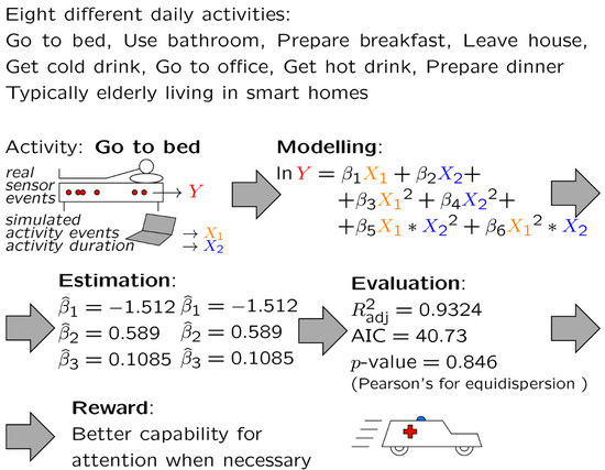
Activity 1: Go to bed

You can stay in bed all the time that you want. Time maximum is 2 min. Then, you have to leave the bedroom, close the door and press the button.

Activity 2: Use bathroom

You can use the toilet if you need, or just wash your hands. Then, leave the bathroom, close the door, and press the button.

Activity 3: Prepare breakfast

You have to prepare something to eat for breakfast. You can choose between milk and cereals or coffee, but you can make or also prepare both. Then, put the bowl on the table, sitting, and press the button.

Activity 4: Leave house

You can choose to leave the home either from the front door or from the garden door. When you are outside, press the button.

Activity 5: Get cold drink

You can choose between tap water or by taking something from the fridge. Then, put the glass with the drink on the kitchen desk and push the button.

Activity 6: Go to Office

You have to go to the office and press the button.

Activity 7: Get hot drink

You can choose between making tea or coffee. Then, put the cup on the kitchen desk and press the button.

Activity 8: Prepare dinner

You have to prepare a soup. Put the bowl on the table and press the button.
Once participants finished the aforementioned activities within the simulator, they were required to undertake the ADLs at HINT. The resulting data from real home and virtual environment were then arranged as two datasets specifying each sensor events aligned with their corresponding participant, sensor ID, code, sensor type, and time stamp. The next chapter will present the comparison between data emanating from HINT and IE Sim in terms of real SEPA. Furthermore, it will illustrate how synthetic data can be transformed (using Poisson regression modelling) for approximating the number of events perceived by each sensor in the real environment.

5. Results and Discussion

5.1. Contrast between Simulated and Real Sensor Events

Paired t-tests ( α = 5% , C L = 95%) were performed to contrast the number of synthetic and real SEPA considering two sensor types: door and pressure. This study also regarded seven ADLs (Go to bed, Use bathroom, Prepare breakfast, Leave house, Get cold drink, Be in the office, and Prepare dinner) and eleven sensors (Bedroom door, Bed pressure, Bathroom door, Bowl cupboard–Prepare breakfast, Refrigerator–Prepare breakfast, Chair pressure–Prepare breakfast, Chair pressure–Leave house, Refrigerator–Get cold drink, Office chair pressure 3, Bowl cupboard–Prepare dinner, Chair pressure–Prepare dinner) for providing further analysis on how the equivalence between real and synthetic datasets may vary depending on the related ADL and sensor type.

5.1.1. Door Sensors: Bedroom Door (ADL: Go to bed)

Figure 3 and Table 2 describe the results obtained from the contrast between synthetic and real SEPA for Bedroom door (ADL: Go to bed). In this case, the two-sided CI for the mean difference between the real and synthetic SEPA does not contain zero (Figure 3), suggesting that, in case of “Bedroom door sensor” (ADL: Go to bed), the SEPA generated by the IE Sim simulator is significantly different from those emanated from the real environment with a confidence level of 95 % . This result is consistent with the small p-value (0.005) derived from the paired t-test which does not provide good evidence for the equivalence statement. Specifically, the real SEPA (mean = 4.125 events) was found to be meaningfully higher than the number of events reported by IE Sim (mean = 1.750 events).
The aforementioned analysis was extended to all door sensors so that further insights can be obtained regarding the equivalence between synthetic data and real observations (refer to Table 3). In particular, we found that in 83.33 % door sensors, the equivalence statement was rejected (p-value < 0.05 ). It can be hence inferred that the SEPA produced by the IE Sim simulator and real-world are considerably dissimilar (CI = 95 % ). It is hypothesized that the difference between the real and simulated sensor activation is due to differences in how individuals interact with objects in the real world versus in the simulation. For example, when entering a room the individual may move through the doorway and then instinctively push the door closed or partially closed. This would trigger an activation of the contact sensor. Conversely in the simulation, the user is abstracted from what is happening in the environment and has to make a concerted effort to interact with each object/sensor. In this case, they may sometimes forget to do so. Meaning the door may open but may not be closed.

5.1.2. Pressure Sensors: Chair Pressure (ADL: Prepare Breakfast)

Figure 4 and Table 4 present the results of the paired t-test supporting the contrast between the SEPA (Chair pressure) from IE Sim and the real environment when preparing breakfast. Considering that the CI for the mean difference between the compared variables does not include zero, there is then not enough support for the equivalence statement (Figure 4). This finding is confirmed by the small p-value (0.004) associated with the null hypothesis, which further suggests (CL = 95 % ), in this case, no statistical similarity between real data and those produced using the simulator. In particular, the real number of SEPA (mean = 1.250 events) was found to be meaningfully lower compared to the SEPA obtained from the IE simulator (mean = 4.875 events).
The outcomes emanating from the comparative analysis are detailed in Table 5. Supported on statistical evidence, it was inferred that in 60 % of the pressure sensors, the equivalence hypothesis was rejected. Hence, it can be deduced that the SEPA derived from IE Sim and real-world are different (CI = 95 % ) in most sensors.

5.2. Predicting Real SEPA Using Simulated Data: The Application of Poisson Regression

Given that the equivalence hypothesis was rejected in most door and pressure sensors (Section 5.1.1), the next step was to define How the synthetic data could be modified to better approximate the real SEPA. Two types of Poisson regression-based models were proposed to deal with this challenge: sensor-based and dummy-variable based. The following sub-sections will illustrate the results obtained from each of these models including validation (overdispersion, normality, and independence of residuals) and assessment of predictive ability R-Sq(adj). It is noteworthy that no regression model was defined for Sensor 7: Bowl cupboard (Prepare dinner) due to lack of sufficient data.

5.2.1. Sensor-Based Poisson Regression Model

Poisson regression models were defined for the above-described sensors by utilizing Minitab 17® statistical package. The resulting equations have been validated (see Section 3.1, Section 3.2 and Section 3.3) for ensuring their applicability in practical scenarios. The use of sensor-based models is proposed given the diversity of ADLs considered in this study. As mentioned above, models with high predictive ability can be used for complementing real datasets and then training algorithms capable of recognizing ADLs accurately.

Sensor 1: Bedroom Door (ADL: Go to Bed)

In this case, the model (9) was concluded to be statistically significant (p-value = 0.000) at an alpha level of 0.05. This means that at least one predictor coefficient is different from 0 as noted in Equation (9). Furthermore, X 1 (simulated events per activity) and interactions including X 2 (simulated activity duration), and X 3 (simulated events per sensor) were found to be significant. Thus, a model considering these terms may be suitable for predicting Y (real events per sensor).
In this case, the predictive ability of the model was concluded to be satisfactory ( R adj 2 = 90.21 % ). Such a model was also found to have the lowest Akaike Information Criterion -AIC (35.57) and is then concluded to strike a superior balance between data fit and its ability to tackle overfitting.
On the other hand, an Anderson-Darling test was undertaken for assessing the normality of residuals (Figure 5). Considering that p-value = 0.338 and A D = 0.366 , it can be assumed that the residuals do not deviate significantly from the normal probability distribution. Also, the independence assumption was validated through an auto-correlation test whose metrics ( M a x | T | = 0.44 ) evidenced no dependence among residuals. Lately, the deviance (p-value = 0.829 ) and Pearson (p-value = 0.846 ) coefficients were used to verify the equidispersion phenomenon. Given that both p-values are higher than the significance level (0.05), this condition is then discarded and the proposed logarithmic equation (Equation (9)) can be suggested for predicting the response variable Y.
ln Y = 0.2778 X 1 0.00678 X 1 X 2 + 0.000033 X 1 X 2 2 + 0.000122 X 2 2 X 3 .

Sensor 2: Bed Pressure (ADL: Go to Bed)

Similar to Sensor 1 Bedroom door (Go to bed), the predictive model (10) was concluded to be statistically significant (p-value= 0) at 0.05. In this case, X 1 (simulated events per activity), X 2 (simulated activity duration), and interactions including X 1 , X 2 , and X 3 (simulated events per sensor) were identified to explain the response variable. Thus, a Poisson-regression-based model incorporating these predictors may be appropriate for obtaining new Y (real events per sensor) observations. Indeed, the predictive ability R-Sq(adj) was calculated to be 93.24 % which ensures reasonable estimations of Y. AIC index (40.73) also validates this conclusion while confirming the good data fit provided by the model.
On a different tack, the Equation (10) was concluded to satisfy the Poisson regression assumptions. First, the normality of residuals was verified through the Anderson-Darling test statistic ( A D = 0.237; p-value = 0.688) and Quantile-Quantile plots (Figure 5). Besides, the auto-correlation was estimated to be ρ ( h ) = 0 ( M a x | T | = 0.61 ) for all h 0 ; thereby supporting the independence of residuals. Ultimately, the Deviance (p-value = 0.721 ) and Pearson (p-value = 0.716 ) statistical tests sustained the equidispersion assumption. Based on these results, the logarithmic equation is concluded to be valid for predicting the real number of sensor (Bed pressure) events when Going to bed.
ln Y = 1.512 X 1 + 0.859 X 2 + 0.1085 X 1 2 0.0272 X 2 2 + 0.001705 X 1 X 2 2 + 0.00355 X 1 2 X 2

Sensor 3: Bathroom Door (Use Bathroom)

The Poisson regression modelling (11) was also found to be suitable (p-value = 0 ) for approximating the real number of events registered by Bathroom door sensor when participants used the bathroom. Indeed, the good data fit was evidenced through the correlation coefficient ( R adj 2 = 95.09 % ) and AIC (30.59).
The quality of the model described in 11 was verified by assessing the assumptions explained in Section 3. First, the homogeneous property of the Poisson equation was confirmed through the Deviance (p-value = 0.987 ) and Pearson (p-value = 0.988 ) tests which were concluded to accept the null hypothesis. The normality distribution of model residuals was evaluated using the Anderson-Darling test and Q Q p l o t s (Figure 5). In this case, the resulting p-value (p-value = 0.756 ) and A D coefficient (0.218) provide enough support for the normality assumption. Ultimately, the covariates were concluded to be uncorrelated within each sample ( M a x | T | = 1.0 ) which confirms the independence property of the model. Being aware of the above-mentioned findings, the Equation (11) is concluded to be valid for predicting the response Y. Of particular interest is the inclusion of X 1 (simulated events per activity) as the only dependent variable capturing Y variations.
ln Y = 0.2869 X 1 + 0.01313 X 1 2

Sensor 4: Refrigerator (Prepare Breakfast)

The use of a Poisson regression model (12) was also appropriate for estimating the real SEPA when participants opening the refrigerator during breakfast preparation (p-value = 0.000 ). Such a finding was checked upon estimating ( R adj 2 = 92.92 % ) and AIC (29.98) which reflect a high performance concerning prediction ability and data fit respectively.
ln Y = 0.001176 X 2 2 0.000013 X 2 3
To justify the use of this model in practical scenarios, Poisson regression assumptions were checked. Initially, the residuals were verified for deviation from normality (Figure 5). In this case, the results (p-value = 0.566 ; A D = 0.271) are in favour of the normality hypothesis. On the other hand, the auto-correlation test was performed to detect potential correlations with Y and residuals from previous models. Given that M a x | T | = 0.82 , dependence among residuals is discarded at a significance level of 0.05. The assessment of the Poisson model also included evaluating the equidispersion property. The Deviance’s (p-value = 0.965 ) and Pearson’s (p-value = 0.965 ) goodness-of-fit statistics concluded against the alternative; therefore, overdispersion phenomenon cannot be sustained. Considering the aforementioned results, the model (Equation (12)) is assumed to be appropriate for predicting the response variable Y. Similar to the previous model, only one variable ( X 2 : Simulated activity duration) was identified as a good predictor of real SEPA in Refrigerator (Prepare breakfast) sensor.

Sensor 5: Chair Pressure (Prepare Breakfast)

In Chair pressure (Prepare breakfast), two interaction terms (including X 1 and X 3 ) were found to be significant at 0.05 and 0.1 respectively: X 1 * X 3 (p-value = 0.049) and X 1 * X 3 2 (p-value = 0.072). Nevertheless, the best predictive model incorporating these variables (13) (Normality: AD = 0.281 p-value = 0.508 (Figure 5); Independence: M a x | T | = 1.45 ; Equidispersion: Deviance [p-value =0.816 and Pearson [p-value = 0.816) was not considered acceptable for estimating the real SEPA in this sensor ( R adj 2 = 56.36 % ). It is then recommended to include other variables explaining the variability of sensor events when sitting on the chair (ADL: Prepare breakfast). Thereby, the predictive ability of the model can be improved for better training activity recognition algorithms focused on this ADL.
ln Y = 0.0563 X 1 X 3 0.00817 X 1 X 3 2

Sensor 6: Chair Pressure (Prepare Dinner)

A p-value = 0.016 confirms that Poisson regression modelling (Equation (14)) is suitable for representing chair pressure sensor events upon preparing dinner. In Equation (14), X 3 (simulated events per sensor) and a quadratic combination between X 1 (SEPA) and X 2 (simulated activity duration) were found to explain part of the response (Y) variability. ( R adj 2 = 73.11 % ) and AIC (11.69) indicate an acceptable ability for predicting the real observations (Y) based on synthetic data ( X 1 , X 2 , and X 3 ).
ln Y = 0.297 X 3 0.000889 X 1 2 X 2
The suitability of the model presented in Equation (14) was validated through the normality, independence, and equidispersion assumptions (see Section 3). On one hand, the Anderson-Darling test revealed that residuals follow a normal distribution (AD = 0.191; p-value = 0.846).On the other hand, the auto-correlation analysis revealed no interdependence among residuals ( M a x | T | = 1.14 ). Ultimately, p-values of Deviance (0.946) and Pearson (0.960) tests evidence no overdispersion within the Poisson distribution ( κ < 0 ). Thus, Equation (14) provides a reasonable approximation of real sensor events when sitting down at a kitchen chair.
Table 6 summarizes the results (prediction performance and validation) of the sensor-based regression models. In this study, most of the models (Equations (9)–(12)) were found to provide excellent predictions of real SEPA while Equations (14) and (13) were concluded to offer acceptable and non-satisfactory transformations of synthetic data respectively.

5.2.2. Poisson Regression Incorporating Dummy Variables

Dummy binary variables were also incorporated into the Poisson regression modelling as an alternative for predicting the real SEPA of any sensor. In this case, these parameters C i denote the presence or absence of a particular sensor i (i = 1, 2, …, 6) which is defined by two specific codes: 1 and 0 correspondingly. The use of these artificial variables then facilitates the application of a standard predictive model that can be adapted to different types of sensors [39]. The dummy variables to be included in the standard Poisson regression model were predefined as follows:
C 1 (Bedroom door - Go to bed): C 1 = 1 if the sensor is Bedroom door - Go to bed, 0 otherwise.
C 2 (Bed pressure - Go to bed): D 2 = 1 if the sensor is Bed pressure - Go to bed, 0 otherwise.
C 3 (Bathroom door - Use bathroom): D 3 = 1 if the sensor is Bathroom door - Use bathroom, 0 otherwise.
C 4 (Refrigerator - Prepare breakfast): C 4 = 1 if the sensor is Refrigerator - Prepare breakfast, 0 otherwise.
C 5 (Chair pressure - Prepare breakfast): C 5 = 1 if the sensor is Chair pressure - Prepare breakfast, 0 otherwise.
C 6 (Chair pressure - Prepare dinner): C 6 = 1 if the sensor is Chair pressure - Prepare dinner, 0 otherwise.
In this case, X 1 (SEPA), X 2 (simulated activity duration), X 3 (simulated events per sensor), C 2 and C 5 were included into the model either in a single or combined form. Table 7 presents the variables with significant influence on real SEPA Y. Equations (15)–(17) (based on three combinations of D 2 and D 5 ) consolidate these terms for predicting the real SEPA of the sensors.
  • D 2 = 0, D 5 = 0
    Y = 0.512 X 1 + 0.4758 X 2 0.00423 X 2 2 + 0.00019 X 1 X 3 2
  • D 2 = 0, D 5 = 1
    Y = 0.512 X 1 + 0.4758 X 2 0.00423 X 2 2 + 0.00019 X 1 X 3 2 0.1086 X 3
  • D 2 = 1, D 5 = 0
    Y = 2.493 + 0.0512 X 1 0.0068 X 2 0.000423 X 2 2 + 0.000019 X 1 X 3 2 .
Table 8 enlists the performance metrics of the above Poisson regression models. Both R 2 (0.9461) and R adj 2 (0.9353) values evidence excellent data fit. In a similar vein, the small difference (0.0108) between these coefficients reveals no overfitting problems. On a different tack, R pred 2 (0.9272) denotes high predictive ability and new observations can be therefore derived for effectively training activity recognition algorithms. This is confirmed by the error standard deviation and PRESS whose values (0.4821 and 10.9856 respectively) are close to 0.
Following this, the normality, equidispersion, and independence properties were assessed for validating the proposed Poisson regression models. Initially, the Anderson-Darling test (see Figure 6) was undertaken for defining whether the residuals follow a normal distribution. The results confirmed the normality hypothesis ( A D = 0.272; p-value = 0.654) with a mean equals to zero. On the other hand, the randomness test revealed no significant auto-correlations among residuals ( M a x | T | = 0.96 ). Indeed, Figure 6 does not evidence the presence of runs nor other non-random patterns. Ultimately, both Pearson (p-value > 0.15) and Deviance (p-value > 0.15) were found to confirm the equidispersion property. The aforementioned outcomes confirm the appropriateness of the dummy-variable-based model for their use in the wild.
Upon analyzing the results derived from Poisson regression models, we propose the application of sensor-based models in Go to bed (Bed pressure), Bathroom door (Use bathroom), and Refrigerator (Prepare breakfast). In contrast, the dummy-variable-based model is suggested for predicting the real SEPA derived from the rest of the sensors. The rationale behind this decision is the superior performance provided by this model ( R pred 2 = 92.72 % ) compared to those resulting from sensor-based models ( 90.21 % , 56.36 % , and 73.11 % ).

6. Conclusions

This paper presented the use of Poisson regression modelling for transforming simulated smart home data to provide an improved approximation of real SEPA. In doing this, synthetic and real data were compared to verify the equivalence hypothesis. This analysis indicated that sensor events per activity produced by the IESim simulator and real-world data do not tend to be statistically equivalent. These results indicate that whilst interactive simulators provide opportunities to facilitate the collection of data in the absence of a real environment, simulated data may not be truly reflective of that collected in the real world.
Results indicated that real SEPA can be better approximated ( R pred 2 = 92.72 % ) if synthetic data is post-processed through Poisson regression incorporating dummy variables. Such model is particularly suggested for predicting the real SEPA derived from three of the sensors cited in this study (Bedroom door - ADL: Go to bed, Chair pressure - ADL: Prepare breakfast, and Chair pressure - ADL: Prepare dinner). On a different tack, Equation (10) ( R pred 2 = 93.24 % ), Equation (11) ( R pred 2 = 95.09 % ), and Equation (12) ( R pred 2 = 92.92 % ) are recommended for training algorithms recognizing three ADLs: Go to bed, Use bathroom, and Prepare breakfast. Further, the real SEPA from sensors Bedroom door, Bed pressure, Bathroom door, Refrigerator, Chair pressure-Prepare breakfast, and Chair pressure-Prepare dinner are well captured by a combination of Poisson modelling with quadratic (see (9)–(11), (14)–(17)) and cubic (see (12) and (13)) covariates.
It is important to note the limitations of this study. In particular, the assessment was carried out using simulated data from one simulator, IESIm. Therefore, it is not possible to tell whether simulated data produced by other simulators would generate the same results. It is also not possible to say whether similar techniques would work with model-based approaches to data simulation. Nonetheless, results from this research highlight the importance of considering the quality of simulated data when modelling solutions for human activity recognition. Future work will investigate the applicability of these findings to data generated by other simulation techniques including both interactive and model-based approaches.
One appealing idea is the ability to use activity data from one person and transform these so that they fit according to the profile of another person. A means to this end could be achievements from the theory of transfer learning [40]. The relationships making this kind of transformation possible has not been covered in this study but remains as an urgent question for future research.

Author Contributions

Conceptualization, M.A.O.-B. and E.J.; methodology, M.A.O.-B. and E.J.; software, M.A.O.-B. and J.S.; validation, M.A.O.-B.; formal analysis, M.A.O.-B. and J.S.; investigation, J.S., M.A.O.-B., P.P., C.N., I.C. and E.J.; resources, C.N., I.C. and M.A.O.-B.; data curation, M.A.O.-B.; writing–original draft preparation, M.A.O.-B., I.C., P.P., C.N. and E.J.; writing–review and editing, M.A.O.-B., I.C., P.P., C.N., E.J. and J.S.; visualization, M.A.O.-B. and E.J.; supervision, C.N., I.C. and M.A.O.-B.; project administration, C.N., M.A.O.-B. and I.C.; funding acquisition, C.N. and I.C. All authors have read and agreed to the published version of the manuscript.

Funding

This research has received funding under the REMIND project Marie Sklodowska-Curie EU Framework for Research and Innovation Horizon 2020, under Grant Agreement No. 734355.

Acknowledgments

The authors would like to thank Giselle Paola Polifroni Avendaño for her valuable support during this research. Also many thanks to Jens Lundström for his helpful comments and previous work in the field.

Conflicts of Interest

The authors declare no conflict of interest.

Abbreviations

The following abbreviations are used in this manuscript:
ADAnderson-Darling
ADLActivities of Daily Living
CIConfidence interval
GPGeneralized Poisson
HINTHalmstad Intelligent Home
IE SimIntelligent Environmental Simulation
IoTInternet of Things
PIRPassive Infrared
QQQuantile-Quantile
RFIDRadio Frequency Identification
SDStatistically different
SEStatistically equivalent
SEPASensor events per activity

References

  1. Ortiz, M.A.; López-Meza, P. Using computer simulation to improve patient flow at an outpatient internal medicine department. In Proceedings of the International Conference on Ubiquitous Computing and Ambient Intelligence, Las Palmas de Gran Canaria, Spain, 29 November–2 December 2016; Springer: Cham, Switzerland, 2016; pp. 294–299. [Google Scholar]
  2. Barrios, M.A.O.; Caballero, J.E.; Sánchez, F.S. A methodology for the creation of integrated service networks in outpatient internal medicine. In Ambient Intelligence for Health; Springer: Cham, Switzerland, 2015; pp. 247–257. [Google Scholar]
  3. Cheng, L.; Nugent, C.D. Human Activity Recognition and Behaviour Analysis, 1st ed.; Chapter Sensor-Based Activity Recognition Review; Springer Nature: Cham, Switzerland, 2019. [Google Scholar]
  4. Ortiz-Barrios, M.A.; Herrera-Fontalvo, Z.; Rúa-Muñoz, J.; Ojeda-Gutiérrez, S.; De Felice, F.; Petrillo, A. An integrated approach to evaluate the risk of adverse events in hospital sector: From theory to practice. Manag. Decis. 2018, 56, 2187–2224. [Google Scholar] [CrossRef] [Green Version]
  5. Rafferty, J.; Nugent, C.D.; Liu, J.; Chen, L. From activity recognition to intention recognition for assisted living within smart homes. IEEE Trans. Hum.-Mach. Syst. 2017, 47, 368–379. [Google Scholar] [CrossRef] [Green Version]
  6. Nugent, C.; Synnott, J.; Gabrielli, C.; Zhang, S.; Espinilla, M.; Calzada, A.; Lundstrom, J.; Cleland, I.; Synnes, K.; Hallberg, J.; et al. Improving the quality of user generated data sets for activity recognition. In Ubiquitous Computing and Ambient Intelligence; Springer: Cham, Switzerland, 2016; pp. 104–110. [Google Scholar]
  7. Helal, S.; Kim, E.; Hossain, S. Scalable approaches to activity recognition research. In Proceedings of the 8th International Conference Pervasive Workshop, Helsinki, Finland, 17–20 May 2010; pp. 450–453. [Google Scholar]
  8. Barrios, M.O.; Jiménez, H.F.; Isaza, S.N. Comparative analysis between ANP and ANP-DEMATEL for six sigma project selection process in a healthcare provider. In International Workshop on Ambient Assisted Living; Springer: Cham, Switzerland, 2014; pp. 413–416. [Google Scholar]
  9. Barrios, M.O.; Jiménez, H.F. Reduction of average lead time in outpatient service of obstetrics through six sigma methodology. In Ambient Intelligence for Health; Springer: Cham, Switzerland, 2015; pp. 293–302. [Google Scholar]
  10. Tapia, E.M.; Intille, S.S.; Larson, K. Activity recognition in the home using simple and ubiquitous sensors. In Proceedings of the International Conference on Pervasive Computing, Vienna, Austria, 21–23 April 2004; Springer: Cham, Switzerland, 2004; pp. 158–175. [Google Scholar]
  11. Cook, D.; Schmitter-Edgecombe, M.; Crandall, A.; Sanders, C.; Thomas, B. Collecting and disseminating smart home sensor data in the CASAS project. In Proceedings of the CHI Workshop on Developing Shared Home Behavior Datasets to Advance HCI and Ubiquitous Computing Research, Boston, MA, USA, 4–9 April 2009; pp. 1–7. [Google Scholar]
  12. Van Kasteren, T.; Noulas, A.; Englebienne, G.; Kröse, B. Accurate activity recognition in a home setting. In Proceedings of the 10th international conference on Ubiquitous computing, Seoul, Korea, 21–24 September 2008; pp. 1–9. [Google Scholar]
  13. Alshammari, N.; Alshammari, T.; Sedky, M.; Champion, J.; Bauer, C. Openshs: Open smart home simulator. Sensors 2017, 17, 1003. [Google Scholar] [CrossRef] [Green Version]
  14. De-La-Hoz-Franco, E.; Ariza-Colpas, P.; Quero, J.M.; Espinilla, M. Sensor-based datasets for human activity recognition–A systematic review of literature. IEEE Access 2018, 6, 59192–59210. [Google Scholar] [CrossRef]
  15. Rafferty, J.; Synnott, J.; Nugent, C.D.; Ennis, A.; Catherwood, P.A.; McChesney, I.; Cleland, I.; McClean, S. A Scalable, Research Oriented, Generic, Sensor Data Platform. IEEE Access 2018, 6, 45473–45484. [Google Scholar] [CrossRef]
  16. Synnott, J.; Nugent, C.; Jeffers, P. Simulation of smart home activity datasets. Sensors 2015, 15, 14162–14179. [Google Scholar] [CrossRef] [PubMed]
  17. Lundström, J.; Synnott, J.; Järpe, E.; Nugent, C.D. Smart home simulation using avatar control and probabilistic sampling. In Proceedings of the 2015 IEEE International Conference On Pervasive Computing And Communication Workshops (Percom Workshops), St. Louis, MO, USA, 23–27 March 2015; IEEE: Piscataway, NJ, USA, 2015; pp. 336–341. [Google Scholar]
  18. Ortiz-Barrios, M.; Lundström, J.; Synnott, J.; Järpe, E.; Sant’Anna, A. Complementing real datasets with simulated data: A regression-based approach. In Multimedia Tools and Applications; Springer: Cham, Switzerland; pp. 1–24.
  19. Schreiber, T.; Schmitz, A. Surrogate time series. Phys. D Nonlinear Phenom. 2000, 142, 346–382. [Google Scholar] [CrossRef] [Green Version]
  20. Maiwald, T.; Mammen, E.; Nandi, S.; Timmer, J. Surrogate data—A qualitative and quantitative analysis. In Mathematical Methods in Signal Processing and Digital Image Analysis; Springer: Cham, Switzerland, 2008; pp. 41–74. [Google Scholar]
  21. Salazar, A.; Safont, G.; Vergara, L. Surrogate techniques for testing fraud detection algorithms in credit card operations. In Proceedings of the 2014 International Carnahan Conference on Security Technology (ICCST), Rome, Italy, 13–16 October 2014; IEEE: Piscataway, NJ, USA, 2014; pp. 1–6. [Google Scholar]
  22. Abroug, F.; Ouanes-Besbes, L.; Elatrous, S.; Brochard, L. The effect of prone positioning in acute respiratory distress syndrome or acute lung injury: A meta-analysis. Areas of uncertainty and recommendations for research. Intensive Care Med. 2008, 34, 1002. [Google Scholar] [CrossRef]
  23. Synnott, J.; Chen, L.; Nugent, C.D.; Moore, G. The creation of simulated activity datasets using a graphical intelligent environment simulation tool. In Proceedings of the 2014 36th Annual International Conference of the IEEE Engineering in Medicine and Biology Society, Chicago, IL, USA, 26–30 August 2014; IEEE: Piscataway, NJ, USA, 2014; pp. 4143–4146. [Google Scholar]
  24. Ariani, A.; Redmond, S.J.; Chang, D.; Lovell, N.H. Simulation of a smart home environment. In Proceedings of the 2013 3rd International Conference on Instrumentation, Communications, Information Technology and Biomedical Engineering (ICICI-BME), Bandung, Indonesia, 7–8 November 2013; IEEE: Piscataway, NJ, USA, 2013; pp. 27–32. [Google Scholar]
  25. Francillette, Y.; Boucher, E.; Bouzouane, A.; Gaboury, S. The Virtual Environment for Rapid Prototyping of the Intelligent Environment. Sensors 2017, 17, 2562. [Google Scholar] [CrossRef] [PubMed] [Green Version]
  26. Park, B.; Min, H.; Bang, G.; Ko, I. The User Activity Reasoning Model in a Virtual Living Space Simulator. Int. J. Softw. Eng. Its Appl. 2015, 9, 53–62. [Google Scholar] [CrossRef]
  27. Lee, J.W.; Cho, S.; Liu, S.; Cho, K.; Helal, S. Persim 3d: Context-driven simulation and modeling of human activities in smart spaces. IEEE Trans. Autom. Sci. Eng. 2015, 12, 1243–1256. [Google Scholar] [CrossRef]
  28. McGlinn, K.; O’Neill, E.; Gibney, A.; O’Sullivan, D.; Lewis, D. SimCon: A Tool to Support Rapid Evaluation of Smart Building Application Design using Context Simulation and Virtual Reality. J. UCS 2010, 16, 1992–2018. [Google Scholar]
  29. Renoux, J.; Klugl, F. Simulating daily activities in a smart home for data generation. In Proceedings of the 2018 Winter Simulation Conference (WSC), Göteborg, Sweden, 9–12 December 2018; IEEE: Piscataway, NJ, USA, 2018; pp. 798–809. [Google Scholar]
  30. Mendez-Vazquez, A.; Helal, A.; Cook, D. Simulating events to generate synthetic data for pervasive spaces. In Workshop on Developing Shared Home Behavior Datasets to Advance HCI and Ubiquitous Computing Research; 2009; Available online: https://pdfs.semanticscholar.org/a7ce/e34ebf272ba18eb60f1a23bd713890890e0c.pdf (accessed on 19 February 2020).
  31. Cameron, A. Regression Analysis of Count Data; Cambridge University Press: Cambridge, UK, 1998. [Google Scholar]
  32. Kunkler, M. Modelling negatives in stochastic reserving models. Insur. Math. Econ. 2006, 38, 540–555. [Google Scholar] [CrossRef]
  33. Andersson, P.K.; Skovgaard, L.T. Regression with Linear Predictors; Springer: Cham, Switzerland, 2010. [Google Scholar] [CrossRef]
  34. Joe, H.; Zhu, R. Generalized Poisson distribution: The property of mixture of Poisson and comparison with negative binomial distribution. Biom. J. 2005, 47, 219–229. [Google Scholar] [CrossRef] [PubMed]
  35. Consul, P.; Famoye, F. Generalized Poisson regression-model. Commun. Stat. Theory Methods 1992, 21, 89–109. [Google Scholar] [CrossRef]
  36. Marsaglia, G. Evaluating the Anderson-Darling Distribution. J. Stat. Softw. 2005, 9, 219–229. [Google Scholar] [CrossRef] [Green Version]
  37. Ljung, G.; Box, G. On a Measure of a Lack of Fit in Time Series Models. Biometrika 1978, 65, 297–303. [Google Scholar] [CrossRef]
  38. Lundström, J.; De Morais, W.O.; Menezes, M.; Gabrielli, C.; Bentes, J.; Sant’Anna, A.; Synnott, J.; Nugent, C. Halmstad intelligent home-capabilities and opportunities. In Proceedings of the International Conference on IoT Technologies for HealthCare, Västerås, Sweden, 18–19 October 2016; Springer: Cham, Switzerland, 2016; pp. 9–15. [Google Scholar]
  39. Nisbet, R.; Elder, J.; Miner, G. Handbook of Statistical Analysis and Data Mining Applications; Academic Press: Cambridge, MA, USA, 2009. [Google Scholar]
  40. Torrey, L.; Shavlik, J. Transfer learning. Handbook of Research on Machine Learning Applications and Trends: Algorithms, Methods, and Techniques; IGI Global: Hershey, PA, USA, 2009. [Google Scholar] [CrossRef] [Green Version]
Figure 1. (Left) The Halmstad Intelligent Home (HINT) kitchen. (Right) The dining and living rooms at Halmstad Intelligent Home.
Remotesensing 12 00771 g001
Figure 2. (Left) User during the first simulation test with IE Sim. (Right) The virtual representation of HINT environment designed within IE Sim.
Remotesensing 12 00771 g002
Figure 3. Contrast between real and simulated sensor events per activity (SEPA)—Bedroom door (Activities of Daily Living (ADL): Go to bed).
Remotesensing 12 00771 g003
Figure 4. Differences between real and simulated SEPA—Chair pressure (ADL: Prepare breakfast).
Remotesensing 12 00771 g004
Figure 5. Normality plots of residuals of real SEPA. The sensors are in the first row from the left: Bedroom door (Go to bed), Bed pressure (Go to bed), in the second row: Bathroom door (Use the bathroom), Refrigerator (Prepare breakfast). in third row: Chair pressure (Prepare breakfast), Chair pressure (Prepare dinner).
Remotesensing 12 00771 g005
Figure 6. QQ-plot and auto-correlation of real SEPA: Poisson regression model with dummy variables.
Remotesensing 12 00771 g006
Table 1. Table summarizing notable works which have produced interactive simulation tools for Smart environments. This highlights the lack of comparison with real world datasets.
AuthorDate2D/3DComparison with Real Data
OpenSHS [13]20173DNo
Park [26]20153DNo
PerSim [27]20153DYes
IE Sim [23]20153DYes
Ariani [24]20132DNo
SimCon [28]20103DNo
Table 2. Comparison test between real and simulated SEPA in Bedroom door (ADL: Go to bed).
VariableMeanStandard dev.S.E. of the Mean
SEPA_Bedroom door_Simulation1.7501.1650.412
SEPA_Bedroom door_Real world4.1251.1260.398
Difference 2.375 1.6850.596
Table 3. Contrast between simulated and real door SEPA.
Sensor–ActivityTwo-Sided CI
for the Mean Difference between
Real and Simulated SEPA (95%)
t-Statisticp-ValueFinding
Bedroom door–Go to bed [ 3.784 , 0.966 ] 3.99 0.005SD
Bathroom door–Use bathroom [ 2.066 , 0.184 ] 2.83 0.026SD
Bowl cupboard–Prepare breakfast [ 0.0 ] 01.0SE
Refrigerator–Prepare breakfast [ 2.682 , 0.318 ] 3.00 0.020SD
Refrigerator–Get cold drink [ 1.721 , 0.864 ] 0.81 0.0448SD
Bowl cupboard–Prepare dinner [ 1.159 , 2.341 ] 7.00 0.000SD
Table 4. Contrast between real and simulated SEPA in Chair pressure (ADL: Prepare breakfast).
VariableMeanStandard dev.Standard Error of the Mean
SEPA_Chair pressure_Synthetic4.8751.8850.666
SEPA_Chair pressure_Real world1.2501.2820.453
Difference 3.625 2.4460.865
Table 5. Comparison between simulated and real pressure sensor events per activity.
Sensor–ActivityTwo-Sided CI
for the Difference between
Real and Simulated SEPA
t-Valuep-ValueConclusion
Bed pressure–Go to bed [ 2.46 , 34.29 ] (90%) 2.19 0.065SD
Chair pressure–Prepare breakfast [ 1.580 , 5.670 ] (95%) 4.19 0.004SD
Chair pressure–Leave house [ 0.62 , 5.37 ] (95%) 1.87 0.103SE
Office chair pressure 3–Be in the office [ 2.45 , 5.31 ] (95%) 0.90 0.403SE
Chair pressure–Prepare dinner [ 2.741 , 5.009 ] (95%) 8.08 0.000SD
Table 6. Of determination coefficient values and model assessment results for the different sensors.
SensorBedroom
door
Bed
pressure
Bedroom
door
RefrigeratorChair
pressure
Chair
pressure
ADLGo to
bed
Go to
bed
Use
bathroom
Prepare
breakfast
Prepare
breakfast
Prepare
dinner
R 2 (adj.)0.90210.93240.95090.92920.56360.7311
AIC35.5740.7330.5929.9819.4411.69
Assessment of Poisson regression model
Auto-correlation
T-statistic
0.440.611.00.821.451.14
Normally distributed residuals
p-value
0.3380.6880.9870.5660.5080.846
Equidispersion
Deviance p-value
0.8290.7210.9870.9650.8160.946
Equidispersion
Pearson p-value
0.8460.7160.9880.9650.8160.960
Table 7. ANOVA results for the dummy-variable based model.
PredictorDFContributionAdj MSF-Valuep-Value
X 1 129.8129.812128.250.000
X 2 13.293.29614.180.001
D 2 16.136.13226.380.000
X 2 2 117.7117.71676.220.000
X 2 D 2 14.404.40518.950.000
X 3 D 5 11.431.4286.150.018
X 3 3 12.892.89212.440.001
Error358.130.232
Total42151
Table 8. Performance indicators of the Poisson regression model with dummy variables.
S R 2 R 2 (adj.) R 2 (pred)PRESS
0.48210.94610.93530.927210.9856

