Quantitative Evaluation of Environmental Loading Induced Displacement Products for Correcting GNSS Time Series in CMONOC

Abstract

Mass redistribution within the Earth system deforms the surface elastically. Loading theory allows us to predict loading induced displacement anywhere on the Earth’s surface using environmental loading models, e.g., Global Land Data Assimilation System. In addition, different publicly available loading products are available. However, there are differences among those products and the differences among the combinations of loading models cannot be ignored when precisions of better than 1 cm are required. Many scholars have applied these loading corrections to Global Navigation Satellite System (GNSS) time series from mainland China without considering or discussing the differences between the available models. Evaluating the effects of different loading products over this region is of paramount importance for accurately removing the loading signal. In this study, we investigate the performance of these different publicly available loading products on the scatter of GNSS time series from the Crustal Movement Observation Network of China. We concentrate on five different continental water storage loading models, six different non-tidal atmospheric loading models, and five different non-tidal oceanic loading models. We also investigate all the different combinations of loading products. The results show that the difference in RMS reduction can reach 20% in the vertical component depending on the loading correction applied. We then discuss the performance of different loading combinations and their effects on the noise characteristics of GNSS height time series and horizontal velocities. The results show that the loading products from NASA may be the best choice for corrections in mainland China. This conclusion could serve as an important reference for loading products users in this region.

1. Introduction

Global Navigation Satellite System (GNSS) is used to monitor both linear and non-linear geodynamic surface displacements. To better understand the geodynamics signals in GNSS, the non-linear variations, which are dominated by environmental loading should first be removed [1,2,3,4,5]. Numerous investigations have addressed the effect of mass loading induced displacements on GNSS coordinate time series. At the global scale, an analysis of baselines determined by Very Long Baseline Interferometry (VLBI), van Dam et al. [6] proved that the weighted root mean square (WRMS) degradation of all baselines were consistent with ~60% of the computed pressure contribution being present in the VLBI length determinations. van Dam et al. also concluded that surface displacements induced by atmospheric pressure changes could account for up to 24% of the total variance in the Global Positioning System (GPS) height estimates [7], and that removing the modeled atmospheric pressure loading from globally distributed GNSS determinations of baseline length for baselines longer than 6000 km reduced the variance on 73 of the 117 baselines investigated. Dong et al. [8] conducted a highly detailed study on the contributors to seasonal terms in position time series from 128 GNSS sites and showed that the seasonal surface mass redistributions account for ~40% of the observed power of the annual vertical variations in site positions. On a basis of global sites, Tregoning et al. [9] documented that the majority of non-tidal deformation can be modeled by applying a daily-averaged correction to daily estimates of coordinates but a greater improvement in height root mean square (RMS) was found if the correction was applied at the observation level. Williams et al. [10] and van Dam et al. [11] concluded that the ocean bottom pressure signal should be considered when accurate geophysical signals from GNSS height coordinates for island and coastal sites are desired.

In terms of regional studies, Deng et al. [12] found that environmental mass distribution accounts for the seasonal signals to a large extent in the vertical displacements of Crustal Movement Observation Network of China (CMONOC) continuous GNSS sites. Yuan et al. [13] investigated the influence of environmental loading corrections predicted by the German Research Centre for Geosciences (GFZ) on the reprocessed coordinate time series of the CMONOC and found that the vertical velocity uncertainties were overestimated by about 1.4 times, on average. In addition, Yuan et al. [14], in another study showed that the GNSS velocity uncertainties were reduced significantly when the common mode components of the time series were spatiotemporally filtered out.

A number of environmental loading predicted displacement products are available from different institutions, i.e., GFZ (http://rz-vm115.gfz-potsdam.de:8080/repository), School and Observatory of Earth Sciences (EOST, http://loading.u-strasbg.fr/) Loading Service from University of Strasbourg and International Mass Loading Service (IMLS, http://massloading.net) from the National Aeronautics and Space Administration (NASA). Different studies have applied different loading models. For example, Ferreira et al. [15] analyzed observations from space-borne geodetic sensors and 3 to 15 years of vertical crustal displacements induced by surface loading models, which were provided by IMLS [16,17], to investigate the seasonal displacements of Earth’s crust. What is more, it has been shown that significant differences exist among different loading products, which most likely result from the different input environmental loading models and the different computational strategies used by these institutions. In an analysis of GNSS time series analysis from the Finnish Antarctic research station, Andrei et al. [18] found that the difference in the vertical component at the ABOA GNSS station between the environmental loading time series provided by GFZ and those from EOST could be up to 3 mm. With environmental mass loading models from EOST, Klos et al. [19] studied 376 International GNSS Service (IGS) International Terrestrial Reference Frame (ITRF2014) stations and found that when the loading models were removed from GNSS data, the uncertainty of velocity decreased. Blewitt and Lavallee [3] concluded that below 2.5 years, the velocity bias becomes unacceptably large when annual signals induced by hydrological and atmospheric loading is not accounted for. The question arises: “How different would the velocity estimate be if a different model had been applied?”.

These results indicate that a thorough evaluation of the effects of these different mass loading products on GNSS time series is required. Jiang et al. [20] conducted a comparative detailed analysis of three different environmental loading methods and their impacts on height time series across 233 globally distributed GNSS stations. They found that the WRMS of the up-coordinate time series was reduced by 74% when the Optimum Model Data (OMD) model was applied, 64% when the Global Geophysical Fluid Center (GGFC) model was applied, and 41% using Loading Model of Quasi-Observation Combination Analysis software (QLM) loading. Li et al. [21] compared weekly GNSS height time series with five continental water storage (CWS) models and found that the higher spatial resolution Modern-Era Retrospective Analysis for Research and Applications (MERRA), CWS product, reduces the scatter of the GNSS height by 2%–6% compared with the Global Land Data Assimilation System (GLDAS). Concentrating on the non-tidal atmospheric pressure loading (NATML) using NASA’s Modern-Era Retrospective Analysis for Research and Applications (MERRA-NATML) and the European Center for Medium-Range Weather Forecasts operational model (ECMWF-NATML), non-tidal ocean loading (NTOL) predicted from the Ocean Model for Circulation and Tides model (OMCT-NTOL), the continental water storage loading (CWSL) predicted from the MERRA model (MERRA-CWSL), and the GFZ’s Land Surface Discharge Model (LSDM-CWSL), Xu [22] evaluated their effects on the scatter of GNSS height time-series from 240 globally distributed sites. They concluded that the MERRA-NATML&OMCT-NTOL&MERRA-CWSL combination reduced the WRMS in 96% (Jet Propulsion Laboratory (JPL) solutions) and 86% (Scripps Orbit and Permanent Array Center (SOPAC) solutions) of the cases, and ECMWF-NATML&OMCT-NTOL&LSDM-CWSL reduced the WRMS in 95% (JPL solutions) and 88% (SOPAC solutions) of the cases.

Although comparisons of some loading products have been made, no systematic comparison of the loading products from GFZ, EOST, and NASA on CMONOC has been conducted to date. The goal of this paper is a thorough evaluation of these different environmental loading models for correcting GNSS coordinate time series. The paper is organized as follows. Section 2 describes the GNSS data sources, publicly available loading products and the methods used to analyze them. Section 3 reports the statistical results from the comparative analysis on the 220 GNSS sites from CMONOC to quantify the performance of three institutions’ loading products and their combinations. Section 4 discusses the influences of different loading products on velocity estimations of GNSS time series. Finally, Section 5 summarizes the main achievements and the work need further study.

2. Data and Methodology

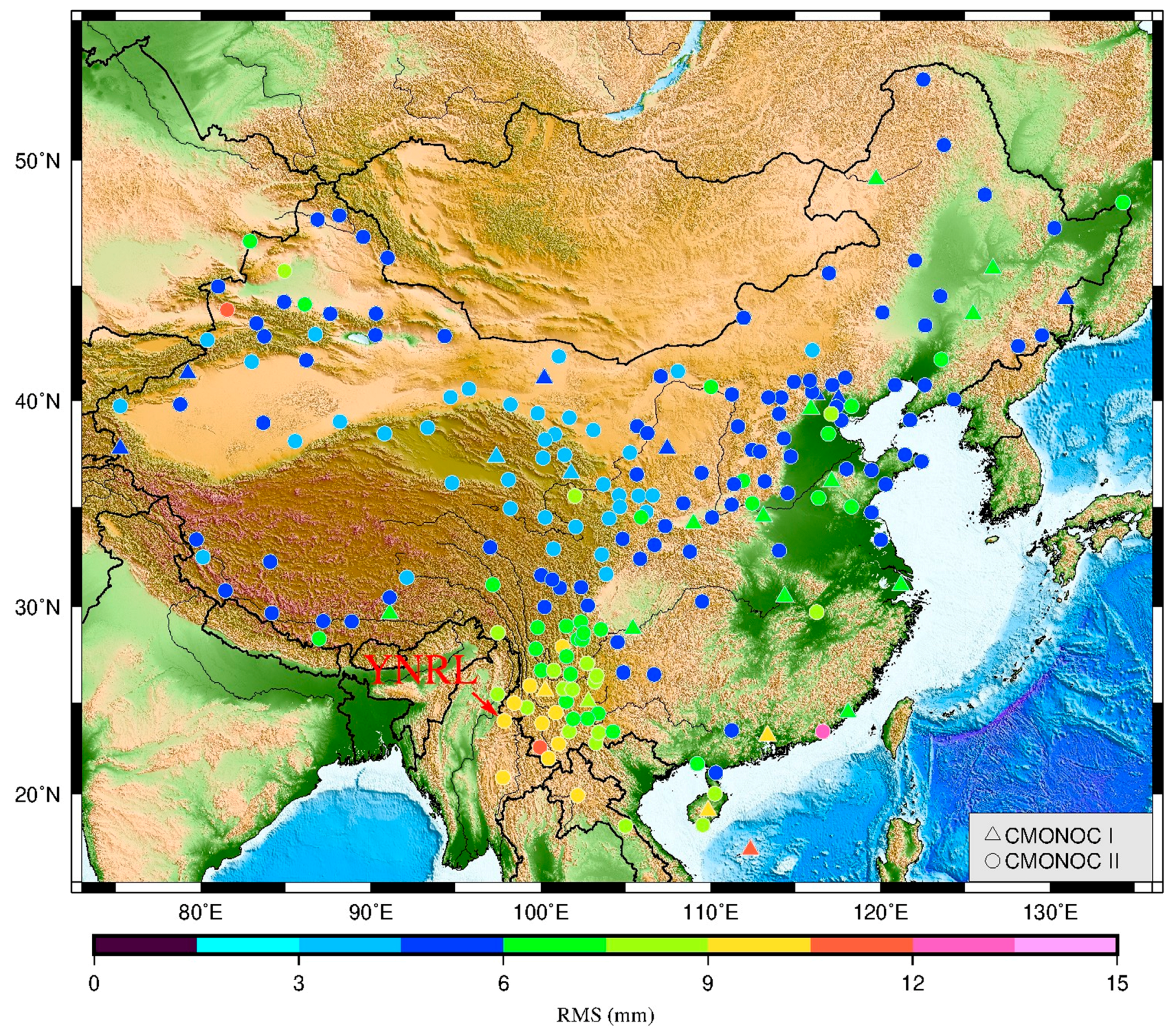
2.1. CMONOC and GNSS Time Series Analysis

The Crustal Movement Observation Network of China is mainly composed of 260 continuous and 2000 irregularly observing stations using GNSS, Very Long Baseline Interferometry (VLBI), Satellite Laser Ranging (SLR), terrestrial gravity, etcetera. Its aim is to monitor crustal movement, the gravity field and its changes, water vapor content in troposphere, and electron density content of the ionosphere over mainland China. CMONOC I began observing in 1999 and CMONOC II in 2010 with the longest time series spanning from 1999 to 2018. Bernese GNSS software [23] was used to homogenously process the GNSS data and a daily loose solution was obtained. The detailed data processing strategies are described in Wu [24]. No observation level non-tidal loading corrections were applied. After adjustment and coordinate transformation the time series were processed further, including outlier elimination, offset and co-seismic jump adjustment, post-seismic relaxation, and trend removal. Afterwards those time series whose time span are longer than 2 years were selected. The 220 stations used in this paper are shown in Figure 1.

To analyze the GNSS time series and characterize optimal noise model after removing outliers and post-seismic relaxation, we use the following equation:

$$y(t_i)=y_0+{vt}_i+{\displaystyle \sum }_{k=1}^q{a}_{k}sin({2\mathsf{\pi }f}_k{t}_i)+b_{k}cos({2\mathsf{\pi }f}_k{t}_i)+{\displaystyle \sum }_{j=1}^{n_g}{g}_j{H(t}_i-T_{g_j})+ϵ{(t}_i)$$

(1)

where $y_0$ is the intercept; $v$ is the linear trend in unit per year, where a year is defined as 365.25 days; $a_k,b_k$ are the amplitude of periodic signals and $f_k$ is the corresponding frequency; $g_j$ and $T_{g_j}$ is the offset and corresponding epoch, respectively; $ϵ$ is the residual (noise) which we pay most attention to; $H$ is the Heaviside step function:

$$\{\begin{array}{c}H(t)=0,t<0\\ H(t)=0.5,t=0\\ H(t)=1,t>0\end{array}$$

(2)

In this study, we used the Hector software [25] to perform the noise analysis for GNSS time series with maximum likelihood estimation (MLE). Although MLE has been known as the most accurate method for the noise analysis [26], a presumed noise model needs to be applied first if we carry out a noise analysis. There are various noise models to choose from in Hector, including power-law noise (PL), white noise (WN), flicker noise (FN), random walk noise (RW), generalized Gauss-Markov noise (GGM), ARMA (1,0) first-order autogressive noise model (AR1), and combinations of these noise models. For example, PLWN means power-law noise plus white noise, which is a common noise combination for the analysis of GNSS coordinate time series. We also used Hector software to eliminate outliers with interquartile range (IQR) criterion.

2.2. Current Existing Environmental Loading Products

Environmental loading estimates due to CWSL, non-tidal atmospheric loading (NTAL), and NTOL for 3D (three dimensional) displacement products are obtained from GFZ, EOST, and NASA. GFZ [27] using the Green’s function approach, as described by Farrell [28], provides hydrological loading products from LSDM forced by ECMWF operational atmospheric data, non-tidal atmospheric loading products from operational ECMWF atmospheric surface pressure and non-tidal oceanic loading (HYDL) products from EMPIOM ocean circulation model forced by ECMWF operational atmospheric data. EOST [29] models the global grids using spherical harmonics formalism and the three dimensional site displacements using refined Green’s functions to compute the elastic deformation, offering various hydrological loading products including ERA interim, GLDAS/Noah, MERRA-land, and Modern-Era Retrospective Analysis for Research and Applications version 2 (MERRA2), non-tidal atmospheric loading products including ECMWF, ERA interim and non-tidal oceanic loading products including Estimating the Circulation and Climate of the Ocean (ECCO1), and ECCO2 (follow-on ECCO, Phase II). NASA [16] provides two loading products for each environmental loading components by using Spherical harmonics and Load Love Numbers (LLN). Not only are the pre-computed series of loading displacements for space geodesy sites accessible, but one can also interpolate time series of 3D displacements for given sites using their global grids. As a result of the differences in temporal resolution of each loading product, the loading time series are averaged into daily epochs after spatially bi-cubic interpolation so as to be consistent with the GNSS time series. It is worth noting that all the products we used are derived in the center of figure frame (CF frame) as our GNSS time series were transformed into ITRF [30,31]. The detailed information of the various loading products and who provides them are shown in

Table 1. Current existing loading products.

Type	Institution	Model used	Spatial/Time	Time span
CWSL	GFZ	LSDM forced by ECWMF [32]	0.5° × 0.5°/24 h	1976–present
	EOST	ERA interim [33]	0.5° × 0.5°/6 h	1979–present
		GLDAS/Noah [34]	0.5° × 0.5°/3 h	2000–2016
	NASA	Global Earth Observing System Forward Processing Instrumental Team (GEOSFPIT) [35]	2′ × 2′/3h	2000–present
		MERRA2 [36]	2′ × 2′/3 h	1980–present
NTAL	GFZ	ECMWF (http://ecmwf.int)	0.5° × 0.5°/3 h	1976–present
	EOST	ECMWF(IB): assuming an inverted barometer ocean response to pressure forcing	0.5° × 0.5°/3 h	2000–present
		ECMWF (assuming a dynamic ocean response to pressure and winds from TUGO-m barotropic model)	0.5° × 0.5°/3 h	2002–2017
		ERA interim	0.5° × 0.5°/6 h	1979–present
	NASA	GEOSFPIT	2′ × 2′/3 h	2000–present
		MERRA2 [37]	2′ × 2′/6 h	1980–2017
NTOL	GFZ	EMPIOM (3 hourly ocean model EMPIOM) [38]	1° × 1°/3 h	1976–present
	EOST	ECCO1 (http://ecco.jpl.nasa.gov)	0.5° × 0.5°/12 h	1993–present
		ECCO2 [39]	0.5° × 0.5°/24 h	1992–2015
	NASA	MPIOM06 (6 hourly ocean model MPIOM)	2′× 2′/3 h	1980–present
		OMCT05 (OMCT: Ocean Model for Circulation and Tides model) [40]	2′×2′/6 h	1980–2017

.

GFZ provides gridded data and shell-scripts to interpolate that data to a certain station location. They also provide a real-time online loading computation service. NASA provides pre-computed series of loading displacements for space geodetic sites, gridded data, and on-demand loading computation service. EOST only provides the displacements for GRGS (GNSS and DORIS) sites and gridded files for interpolation by users who need them.

To have a general impression of loading effects over CMONOC, Figure 2 shows time series of all loading products and corresponding GNSS time series at YNRL (24.0°N, 97.8°E), which is located in the southwest of the Yunnan province in China (The site is highlighted in Figure 1). We selected this station as our example because of its continuous GNSS time series and relatively strong combined mass loading signals. As shown in the top panel in Figure 2, the hydrological loading induced displacements all show a significant annual variation. The meteorological data (http://data.cma.cn/) indicate that annually this region received on average (2010–2016) 1400 mm of precipitation. The middle panels display the NTAL and NTOL loading signals showing much small magnitudes. The bottom panel SUML shows the sum of CWSL, NTAL, and NTOL products, which usually is taken into consideration when applying loading correction. As shown in Figure 2, loading induced displacements are correlated with GNSS height time series except for the NTOL products because of their small amplitudes. Further, most of the displacements derived from the different centers and input data share the same annual variation. The annual amplitude is about 15 mm.

2.3. Evaluation Metrics

In this study, two metrics, i.e., correlation and RMS reduction were used to evaluate the performance of different environmental loading products. Before calculating these metrics, a linear trend was removed from the loading displacements and GNSS time series. The RMS reduction was calculated by the following equation [41,42]:

$${\mathrm{RMS}}_{\mathrm{reduction}}(\%)=\frac{{\mathrm{RMS}}_{\mathrm{original}}{-\mathrm{RMS}}_{\mathrm{corrected}}}{{\mathrm{RMS}}_{\mathrm{original}}}\times 100$$

(3)

in which ${\mathrm{RMS}}_{\mathrm{original}},{\mathrm{RMS}}_{\mathrm{corrected}}$ are the RMS of GNSS time series before and after applying loading correction, respectively. The RMS reduction serves as an indicator of how much signal from loading models can be explained by the loading time series. The higher RMS reduction values, the better performance of the loading models. If the loading model increases the scatter in the GNSS time series, the RMS reduction will be negative.

In addition, dilution of precision (DP) is adopted as an index to quantify the difference in the velocity uncertainty derived after applying the loading correction. DP is the ratio between uncertainties of velocity estimated before and after applying loading correction, and it is defined as [3,19]:

$$\mathrm{DP}=\frac{{\mathsf{\sigma }}_{\mathrm{c}}}{{\mathsf{\sigma }}_{\mathrm{g}}}$$

(4)

where ${\mathsf{\sigma }}_{\mathrm{c}}$ indicates the velocity uncertainty of GNSS time series with loading correction and ${\mathsf{\sigma }}_{\mathrm{g}}$ means that of original time series. If DP is greater than 1, the velocity uncertainty of GNSS time series increases after applying loading correction.

3. Results

3.1. Comparison of CWSL, NTAL, and NTOL Products

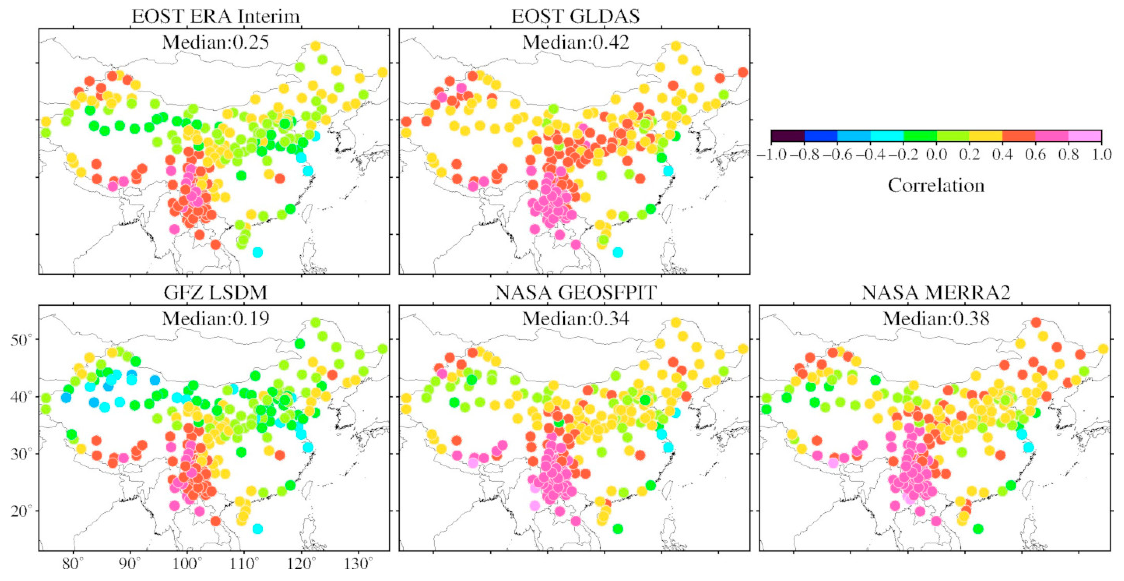
3.1.1. CWSL Products

The correlations and RMS reductions among the different loading model derived displacements and GNSS time series were calculated. For brevity, as the vertical displacement signal is generally stronger than the horizontals, only the results in the vertical component are shown in Figure 3 and Figure 4. The five hydrological loading products show a similar pattern over China in the displacement predicted for the vertical component. Strong correlations and the largest RMS reductions are observed in the southwest of China; the weakest agreement appears in stations in the coastal regions and northwest China where the hydrological signals are weaker. The south of China is influenced by the humid subtropical monsoon climate and the north belongs to monsoon climate of medium latitudes with the border between the south and north in latitude ~34°N (Qingling mountains-Huaihe River) [43]. In addition, the southwest of China is drained by six major river systems, including the Jinsha Jiang, Perl River, Mekong, etc. which greatly increase the supply of water to this region. The RMS of total water storage signal from GLDAS Noah (2002–2017) are given in the Appendix A (Figure A1).

As shown in the Figure 4, the RMS of the GNSS time series is most reduced after applying the EOST-GLDAS product, with a median RMS reduction of 6.56%. Applying the GFZ-LSDM product to the GNSS time series increases the scatter on the observations with a negative median RMS reduction of −1.34%. Please note the results for the stations in Qaidam Basin and north China plain. The RMS reduction of GNSS time series is 5% on average after applying EOST-GLDAS induced displacements, while it is negative for the other four products.

To evaluate the performance of the different loading products with respect to one another,

Table 2. Vertical median RMS reduction difference of CWSL products (%).

	GFZ -LSDM	EOST -ERA Interim	EOST -GLDAS	NASA -GEOSFPIT	NASA -MERRA2
GFZ-LSDM	--	−3.63	−7.81	−7.79	−8.63
EOST-ERA Interim	--	--	−4.18	−4.16	−5.00
EOST-GLDAS	--	--	--	0.03	−0.82
NASA-GEOSFPIT	--	--	--	--	−0.85
NASA-MERRA2	--	--	--	--	--

shows the vertical median RMS reduction difference between each model. As shown in the table, the difference between GFZ-LSDM and NASA-MERRA2 is the largest and that between EOST-GLDAS and NASA-Global Earth Observing System Forward Processing Instrumental Team (GEOSFPIT) is the smallest, with values are −8.63% and 0.03%, respectively. Moreover, as shown in the Table 2, the hydrological loading products that from EOST and NASA are better than those from GFZ, as all the values are negative when GFZ-LSDM is in the comparison. Further, the NASA-MERRA2 model shows the best performance as evidenced by the fact that the values are all negative. It is worth noting, that the EOST-GLDAS, NASA-GEOSFPIT, and NASA-MERR2 show almost no difference as the values of the median RMS reduction difference among these products are less than 1% (0.03%, −0.82%, −0.85%).

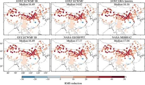
3.1.2. NTAL Products

When we look at the models with respect to the GNSS vertical observations, the RMS reduction not only reflects the phase difference between the two time series, but also the amplitude difference. In this section, only the RMS reductions will be considered in the analysis of NTAL. The correlations between NTAL products and vertical coordinate time series are given in the Appendix A (Figure A2).

Figure 5 shows the RMS reduction of the GNSS vertical scatter as a result of applying the (six) NTAL products. Generally, the performance of the NTAL models increases along with the increase of latitudes of the stations. This is due to the fact that atmospheric pressure signals are more significant in the middle-to-high latitudes than the equator and lower latitudes. More specifically, the average RMS reduction in northern stations (latitude >34°N) is about 30% amplitude of the scatter, whereas that in southern part (latitude <30°N) is about 5% amplitude of the scatter. The root cause is probably the high atmospheric change induced by monsoon in subtropical region. As shown by the median value in the figure, apparently the GNSS time series corrected by GEOSFPIT loading product show marginally better results over the other atmospheric loading products. It is worth mentioning that at station JXHK in Jiujiang and XZCY in Linzhi and several stations in coastal region marked in light blue, the RMS reductions are negative. Bad correlations at the GPS sites close to the coastline are found in other studies which are possibly affected by non-tidal oceanic loading effects [44,45,46] or even spurious long-period signals due to unmodeled short-periodic displacements [47].

Table 3. Vertical median RMS reduction difference of NTAL products (%).

	GFZ-ECWMF	EOST-ECWMF_IB	EOST-ECWMF	EOST-ERA Interim	NASA-GEOSFPIT	NASA-MERRA2
GFZ-ECWMF	--	0	1.67	0.33	−0.68	−0.55
EOST-ECWMF_IB	--	--	1.66	0.33	−0.68	−0.56
EOST-ECWMF	--	--	--	−1.34	−2.35	−2.22
EOST-ERA Interim	--	--	--	--	−1.01	−0.88
NASA-GEOSFPIT	--	--	--	--	--	0.13
NASA-MERRA2	--	--	--	--	--	--

illustrates the performance of different loading products with respect to one another. The observed difference is quite small as the values of the median RMS reduction of the differences are less than 3%, indicating that the differences are not significant when different NTAL products are used to correct the GNSS height time series. However, the relatively large difference (−2.35%) exists between the EOST-European Center for Medium-Range Weather Forecasts (ECWMF) and NASA-GEOSFPIT product possibly because the pressure data sets they used are different. Further, the performance between EOST-ECWMF and NASA-MERRA2 has the secondly big difference in correcting GNSS time series, which is −2.22% according to the table. Note that the NASA-GEOSFPIT has the best performance after applying non-tidal atmospheric loading correction as all the values of that column are negative and the last value of last column is positive as shown in Table 3.

It is worth noting that the station NMAZ (38.8°N, 105.7°E), located in the north of China’s autonomous region—Inner Mongolia, has its RMS reduced most after applying the displacements induced by the NASA-GEOSFPIT product. GEOSFPIT is the best in terms of correcting non-tidal atmospheric loading effect. As shown in Figure 2, the displacements at this station reach their highest point with annual variation of up to 6 mm in annual amplitude as well as the GNSS time series.

3.1.3. NTOL Products

In this section, we present the RMS reductions after applying non-tidal oceanic loading induced displacement corrections. The RMS reductions of GNSS vertical coordinate time series are given in Figure 6. As shown in figure, the RMS reductions have a different performance pattern corrected by the five loading model products, among which NASA-OMCT05 shows the greatest effect as the number of stations had their RMS reduced is the most (dots marked in red) and the median RMS reduction is the biggest.

After applying the ECCO1 product induced displacement corrections, the coordinate time series of stations located in northwest and northeast China have their RMS increased, which are marked in light blue in Figure 6. Meanwhile, this happens in southwest China in the case of ECCO2 products. Whereas, the negative results mostly center on stations around China’s Bohai Bay for GFZ-EMPIOM and NASA-MPIOM06 products. Increased RMS reductions for the five products around China’s Bohai Bay may indicate that the loading induced displacements are poorly modeled here due to the confining coastal geography.

Table 4. Vertical median RMS reduction difference of NTOL products (%).

	GFZ -EMPIOM	EOST -ECCO1	EOST -ECCO2	NASA -MPIOM06	NASA -OMCT05
GFZ-EMPIOM	--	−0.46	−0.51	−0.19	−0.73
EOST-ECCO1	--	--	0.05	−0.66	−1.20
EOST-ECCO2	--	--	--	−0.71	−1.24
NASA-MPIOM06	--	--	--	--	−0.54
NASA-OMCT05	--	--	--	--	--

illustrates the differences in performance of the different loading products with respect to one another. As shown in the table, the GNSS height time series have the biggest RMS reduction difference after applying NTOL correction between EOST-ECCO2 and NASA-OMCT05 product with the value of −1.24%. While the smallest difference is 0.05%, which is the different performance between EOST-ECCO1 and EOST-ECCO2 product. On the whole, the products from NASA have the slight advantage over other products that come from GFZ and EOST as all the values of the last two columns are negative, one of which is NASA-OMCT05 and it is better than the other one. Although the vertical median RMS reduction difference is very small, the RMS reduction difference between GFZ-EMPIOM and NASA-OMCT05 can be up to 10% at stations in Liaodong Peninsula (39°N 119°E/41°N 125°E).

3.2. Optimal Combination of Environmental Loading Models

In this section, we quantitatively evaluate the combination of the three types of loading induced displacements, CWSL, NTAL, and NTOL. Excluding the internal combinations from each institute (one internal combination of GFZ, twelve internal combinations of EOST and eight internal combinations of NASA), we also create all possible combinations of loading products from the different institutions. We analyze 150 different combinations in total. We rank the combinations in terms of the median of RMS reduction. We then selected the best and worst combinations of the internal combinations and the cross-institute combinations. As a result, seven combinations were selected for discussion, which are shown in

Table 5. Statistics of vertical RMS reduction of selected combination (%).

Combination	Alias	Max	Min	Median	Mean	Positive
GFZ-LSDM &GFZ-ECWMF(IB)&GFZ-EMPIOM(IB)	A	38.11	−11.28	23.63	22.8	98.18
EOST-GLDAS &EOST-ECWMF(IB )&EOST-ECCO1	B	44.19	−11.12	26.78	24.93	98.18
NASA-MERRA2 &NASA-GEOSFPIT&NASA-OMCT05	C	42.63	−12.12	26.46	25.19	97.73
NASA-MERRA2 &EOST-ECWMF(IB)&EOST-ECCO2	D	42.82	−13.22	26.91	25.42	98.64
GFZ-LSDM &EOST-ECWMF&EOST-ECCO1	E	38.29	−34.47	22.43	20.66	95.00
EOST-ERA interim &EOST-ECWMF&EOST-ECCO1	F	39.92	−31.02	24.26	22.22	94.55
NASA-GEOSFPIT &NASA-MERRA2&NASA-MPIOM06	G	44.67	−12.94	25.97	24.53	97.73

. To better represent the selected combinations in our following analysis, we simply use uppercase letters A–G to denote the different combinations. For example, A stands for the internal combination of the GFZ loading products. Conservation of mass between the atmosphere, oceans, and continental water are not considered when we combine different types of loading models.

As in the previous sections, only the vertical calculations are presented here. Table 5 shows any model combinations for which more than 94% (207 out of 220) stations have a positive RMS reduction. Combinations A-C represent the institute specific internal combinations. Combinations D-G represent the cross institute combinations. The best combination (D) comes from the combination of NASA-MERRA2, EOST-ECWMF (IB) and EOST-ECCO2 with a median RMS reduction up to 26.91%. While the worst combination (E) is also a cross-institutional combination, i.e. the sum of GFZ-LSDM, EOST-ECWMF and EOST-ECCO1, whose median RMS reduction is 22.43%. With respect to the internal combinations, the median of RMS reduction percentages of the best combination of GFZ, EOST and NASA are 23.63%, 26.78%, and 26.46%, respectively.

Histograms of RMS reductions of the seven combined models are shown in Figure 7. It is clear that all the models demonstrate similar RMS reduction distributions over China. More specifically, the combination C and D shows more stations with RMS reductions bigger than 20% resulting slightly higher median and mean RMS reductions from these two combinations. It is worth noting, that there are several stations that have their RMS increased after applying any combined model loading corrections. This is probably due to the fact that we do not consider conservation of mass between the models.

From the analysis of Section 3.1, we have learned that the best products from each category for correcting the GNSS height time series from CMONOC are EOST-GLDAS (HYDL), NASA-GEOSFPIT (NTAL) and NASA-OMCT05 (NTOL), respectively. However, when these models are combined, the resulting RMS reduction was not the optimal of all the combinations explaining why the supposed best combination is not shown in Table 5. One possible explanation might be that combination of individual best models might result in worse mass conservation problem.

Table 6. Vertical median RMS reduction difference of selected combinations (%).

	A	B	C	D	E	F	G
A	--	−3.15	−2.83	−3.28	1.20	−0.63	−2.34
B	--	--	0.32	−0.13	4.35	2.52	0.81
C	--	--	--	−0.45	4.03	2.20	0.49
D	--	--	--	--	4.48	2.65	0.94
E	--	--	--	--	--	−1.83	−3.54
F						--	−1.71
G							--

shows the median RMS reduction difference with respect to each combination. As shown in the table, the largest difference (4.48%) exists between the D and E combination, which are respectively the best and worst combination of the ‘best’ seven combinations. The smallest difference (−0.13%) exists between the B and D combination, which are respectively the best internal combination of EOST and the best cross-institute combination.

To solve the mass conservation problem when combining the CWSL, NTAL, and NTOL models, GFZ (http://rz-vm115.gfz-potsdam.de:8080/repository/entry/show?entryid=86facac5-2ba3-4ae3-8f3d-4ff972302098) provides the so-called sea-level loading (SLEL) product to make the mass conservative. We added this product to the GFZ’s internal combination and recomputed the combination results, but we find no significant difference by adding the SLEL product.

4. Discussion

4.1. Effects of Different Environmental Loading Products on Noise Characterization

Published research indicates that velocity uncertainty estimates are significantly different among GNSS time series after applying different loading products [48,49]. Therefore, the effects of the different mass loading models on the velocity error estimates should be considered. Figure 8 displays the best noise model by percentage (the noise models considered here include power law (PL), flicker (FN), the combination of flicker noise and white noise (FNWN) of the original GNSS time series. In terms of the selection of best noise model, the Bayesian Information Criterion (BIC) [50] was employed, which were widely used among the geophysical community [51,52,53]. In addition, shown are the noise models of the five combination loading models corresponding to the models listed in Table 2. (Please note that the noise models with less than 10% were summed into the category “Others”). The meaning of capital letters refer to Table 5 in Section 3.2.

As shown in Figure 8, a combination of flicker noise and the white noise is the best noise model in the original GNSS vertical component. This result is consistent with previously published results [26,54,55,56,57,58,59,60,61]. However, power law noise is the second-best noise model. These two noise models represent 71.4% of the noise in the GNSS height time series considered here.

After applying the different loading corrections to the GNSS time series, the dominant noise model varies depending on the loading correction applied. For example, PL noise, which represents the second most dominant model in the original vertical GNSS time series, dominates the noise characteristics when corrected by the loading models. As shown in Figure 8, apart from the GFZ combination, the most dominant model describing the corrected GNSS up coordinate time series is the power law noise. In the cases of combination of GFZ (A) and best combination of NASA (C), the difference between FNWN and PL is marginal, 1.8% versus 3.6%, respectively. Notice that in these two cases the percentage of the combination of FN and WN varies little with the applied loading corrections, whereas the percentage decreased by 10% in other combination solutions. The reasons for this difference need further research in the future.

4.2. Effects of Different Environmental Loading Products on Velocity Estimation

The effects of loading models on GNSS velocity estimates need to be considered because of error propagation [11,62]. To illustrate the difference in velocity before and after applying loading corrections, the differences in horizontal velocity between original GNSS time series and those corrected were calculated. These results are shown in the following figures. Only horizontal velocities are discussed in this section. The horizontal velocity fields presented here are given in ITRF14 and are of the same order of magnitude as the official results (http://www.cgps.ac.cn/cgs/viewArticleNormal.action?id=101).

Figure 9, Figure 10, and Figure 11 show the horizontal velocity fields before and after applying loading correction using the D combination, i.e., NASA-MERRA2, EOST-ECWMF_IB, and EOST-ECCO2. As shown in Figure 10, using the GFZ combination, there is little difference (<0.5 mm/yr) in both magnitude and direction of the velocities. While when the GNSS time series were corrected by other loading models, for example, the D combination, the velocity differences at many stations are significant up to 2 mm/yr on average, where the largest difference is ~3 mm/yr. Additional results of difference in velocity fields before and after applying the loading corrections with other loading combinations are given in Appendix A (Figure A3, Figure A4, Figure A5, Figure A6 and Figure A7).

According to Equation (4), dilution of precision (DP) quantifies the changes of velocity uncertainties. The results of the horizontal velocity with combined loading corrections are illustrated in Figure 12. The smaller the DP, the better the applied loading correction to the GNSS time series. As shown in the figure, the distribution of DP has no apparent tendency over the country. At most stations the dilution of precision is marginally bigger than 1 in the cases of B, D, E, and F, while in the cases of A, C, and G the number of stations with dilution of precision smaller than 1 is slightly more than that bigger than 1. When we refer to the RMS reduction, the C combination with 26.46% median reduction is the highest one among the A, C, G combinations. Therefore, among the seven combinations listed in Table 2, the C combination is recommended for apply loading corrections to GNSS time series over the study region.

5. Conclusions

The goal of this study was to provide a comprehensive comparison of different environmental loading models over the mainland of China using GNSS coordinate time series from CMONOC. We observe significant differences among three different loading models, which have an impact on the noise characteristics of GNSS time series and velocity estimates. The difference in RMS reduction of GNSS time series before and after applying different NTAL products can be up to 15%, and in the case of combination loading correction the difference, up to 20%. This difference cannot be ignored in interpreting high-precision geodetic data.

In addition, the horizontal velocity can be very different when different loading models are applied to GNSS time series. When the GFZ loading combination corrections were used, the difference in horizontal velocity field changed less than 0.5 mm/yr; while in the case of the optimal combination, the difference can be up to 3 mm/yr.

Some loading studies over China have used loading products from GFZ. As shown in the present study, loading products from NASA instead of GFZ may be a better choice for correcting GNSS time series over mainland China although products from GFZ are much easier to be obtained and processed. As far as the RMS reduction is concerned, the B and D combinations (B: EOST-GLDAS&EOST-ECWMF_IB&EOST-ECCO1; D: NASA-MERRA2&EOST-ECWMF_IB&EOST-ECCO2) are recommended for use when correcting the GNSS time series. However, when considering dilution of precision, the C combination (NASA-MERRA2&NASA-GEOSFPIT&NASA-OMCT05) is recommended to correct GNSS time series in mainland China as it could improve the precision of velocity to a better extent.

Nevertheless, the conclusion of this study does not apply to other regions of the world. It is highly recommended that all the available loading models are tested and that the optimal model is chosen for your GNSS time series interpretation.

References

1. Jiang, W.; Xia, C.; Li, Z.; Guo, Q.; Zhang, S. Analysis of Environmental Loading Effects on Regional GPS Coordinate Time Series. Acta Geod. Cartogr. Sin. 2014, 43, 1217–1223. [Google Scholar] [CrossRef] [Green Version]
2. Blewitt, G.; Lavallée, D.; Clarke, P.; Nurutdinov, K. A new global mode of earth deformation: Seasonal cycle detected. Science 2001, 294, 2342–2345. [Google Scholar] [CrossRef] [PubMed] [Green Version]
3. Blewitt, G.; Lavallée, D. Effect of annual signals on geodetic velocity. J. Geophys. Res. Solid Earth. 2002, 107, ETG-9. [Google Scholar] [CrossRef] [Green Version]
4. Jiang, W.; Yuan, P.; Chen, H.; Cai, J.; Li, Z.; Chao, N.; Sneeuw, N. Annual variations of monsoon and drought detected by GPS: A case study in Yunnan, China. Sci. Rep. 2017, 7, 1–10. [Google Scholar] [CrossRef]
5. Pan, Y.; Shen, W.B.; Shum, C.K.; Chen, R. Spatially varying surface seasonal oscillations and 3-D crustal deformation of the Tibetan Plateau derived from GPS and GRACE data. Earth Planet. Sci. Lett. 2018, 502, 12–22. [Google Scholar] [CrossRef]
6. van Dam, T.M.; Herring, T.A. Detection of atmospheric pressure loading using very long baseline interferometry measurements. J. Geophys. Res. Solid Earth. 1994, 99, 4505–4517. [Google Scholar] [CrossRef]
7. van Dam, T.M.; Blewitt, G.; Heflin, M.B. Atmospheric pressure loading effects on Global Positioning System coordinate determinations. J. Geophys. Res. Solid Earth 1994, 99, 23939–23950. [Google Scholar] [CrossRef]
8. Dong, D.; Fang, P.; Bock, Y.; Cheng, M.K.; Miyazaki, S. Anatomy of apparent seasonal variations from GPS-derived site position time series. J. Geophys. Res. Solid Earth. 2002, 107, ETG-9. [Google Scholar] [CrossRef] [Green Version]
9. Tregoning, P. Atmospheric pressure loading corrections applied to GPS data at the observation level. Geophys. Res. Lett. 2005, 32, 1–4. [Google Scholar] [CrossRef] [Green Version]
10. Williams, S.D.P.; Penna, N.T. Non-tidal ocean loading effects on geodetic GPS heights. Geophys. Res. Lett. 2011, 38, 3–7. [Google Scholar] [CrossRef] [Green Version]
11. van Dam, T.; Collilieux, X.; Wuite, J.; Altamimi, Z.; Ray, J. Nontidal ocean loading: Amplitudes and potential effects in GPS height time series. J. Geod. 2012, 86, 1043–1057. [Google Scholar] [CrossRef] [Green Version]
12. Deng, L.; Jiang, W.; Li, Z.; Chen, H.; Wang, K.; Ma, Y. Assessment of second- and third-order ionospheric effects on regional networks: case study in China with longer CMONOC GPS coordinate time series. J. Geod. 2017, 91, 207–227. [Google Scholar] [CrossRef]
13. Yuan, P.; Li, Z.; Jiang, W.; Ma, Y.; Chen, W.; Sneeuw, N. Influences of environmental loading corrections on the nonlinear variations and velocity uncertainties for the reprocessed global positioning system height time series of the crustal movement observation network of China. Remote Sens. 2018, 10, 958. [Google Scholar] [CrossRef] [Green Version]
14. Yuan, P.; Jiang, W.; Wang, K.; Sneeuw, N. Effects of spatiotemporal filtering on the periodic signals and noise in the GPS position time series of the Crustal Movement Observation Network of China. Remote Sens. 2018, 10, 1472. [Google Scholar] [CrossRef] [Green Version]
15. Ferreira, V.G.; Montecino, H.D.; Ndehedehe, C.E.; del Rio, R.A.; Cuevas, A.; de Freitas, S.R.C. Determining seasonal displacements of Earth’s crust in South America using observations from space-borne geodetic sensors and surface-loading models. Earth Planets Sp. 2019, 71, 84. [Google Scholar] [CrossRef] [Green Version]
16. Petrov, L. The international mass loading service. Int. Assoc. Geod. Symp. 2017, 146, 79–83. [Google Scholar]
17. Petrov, L.; Boy, J.-P. Study of the atmospheric pressure loading signal in very long baseline interferometry observations. J. Geophys. Res. Solid Earth. 2004, 109, 1–14. [Google Scholar] [CrossRef] [Green Version]
18. Andrei, C.O.; Lahtinen, S.; Nordman, M.; Näränen, J.; Koivula, H.; Poutanen, M.; Hyyppä, J. GPS time series analysis from Aboa the Finnish Antarctic research station. Remote Sens. 2018, 10, 1937. [Google Scholar] [CrossRef] [Green Version]
19. Klos, A.; Gruszczynska, M.; Bos, M.S.; Boy, J.P.; Bogusz, J. Estimates of Vertical Velocity Errors for IGS ITRF2014 Stations by Applying the Improved Singular Spectrum Analysis Method and Environmental Loading Models. Pure Appl. Geophys. 2018, 175, 1823–1840. [Google Scholar] [CrossRef]
20. Jiang, W.; Li, Z.; van Dam, T.; Ding, W. Comparative analysis of different environmental loading methods and their impacts on the GPS height time series. J. Geod. 2013, 87, 687–703. [Google Scholar] [CrossRef]
21. Li, Z.; van Dam, T.; Collilieux, X.; Altamimi, Z.; Rebischung, P.; Nahmani, S. Quality Evaluation of the Weekly Vertical Loading Effects Induced from Continental Water Storage Models. IAG 150 Years. Int. Assoc. Geod. Symp. 2015, 143, 45–54. [Google Scholar]
22. Xu, C. Evaluating mass loading products by comparison to GPS array daily solutions. Geophys. J. Int. 2017, 208, 24–35. [Google Scholar] [CrossRef]
23. Dach, R.; Lutz, S.; Walser, P.; Fridez, P. Bernese GNSS Software Version 5.2. User manual; University of Bern: Bern, Switzerland, 2015. [Google Scholar]
24. Wu, W. High-precision GPS data processing and contemporary crustal deformation in China mainland. Ph.D. thesiS, Tongji University, Shanghai, China, 2018. [Google Scholar]
25. Bos, M.S.; Fernandes, R.M.S.; Williams, S.D.P.; Bastos, L. Fast error analysis of continuous GNSS observations with missing data. J. Geod. 2013, 87, 351–360. [Google Scholar] [CrossRef] [Green Version]
26. Zhang, J.; Bock, Y.; Johnson, H.; Fang, P.; Williams, S.; Genrich, J.; Wdowinski, S.; and Behr, J. Southern California Permanent GPS Geodetic Array: Error analysis of daily position estimates and site velocities. J. Geophys. Res. Solid Earth. 1997, 102, 18035–18055. [Google Scholar] [CrossRef]
27. Dill, R.; Dobslaw, H. Numerical simulations of global-scale high-resolution hydrological crustal deformations. J. Geophys. Res. Solid Earth. 2013, 118, 5008–5017. [Google Scholar] [CrossRef]
28. Farrell, W.E. Deformation of the Earth by surface loads. Rev. Geophys. 1972, 10, 761–797. [Google Scholar] [CrossRef]
29. Gegout, P.; Boy, J.P.; Hinderer, J.; Ferhat, G. Modeling and Observation of Loading Contribution to Time-Variable GPS Sites Positions. Int. Assoc. Geod. Symp. 2010, 135, 651–659. [Google Scholar]
30. Dong, D.; Yunck, T.; Heflin, M. Origin of the International Terrestrial Reference Frame. J. Geophys. Res. Solid Earth 2003, 108, 1–10. [Google Scholar] [CrossRef]
31. Blewitt, G. Self-consistency in reference frames, geocenter definition, and surface loading of the solid Earth. J. Geophys. Res. Solid Earth 2003, 108(B2). Available online: https://doi.org/10.1029/2002JB002082 (accessed on 9 February 2020). [CrossRef] [Green Version]
32. Dill, R. Hydrological model LSDM for operational Earth rotation and gravity eld variations. Sci. Tech. Rep. 08/09 2008, 369. Available online: https://doi.org/10.2312/GFZ.b103-08095 (accessed on 9 February 2020). [CrossRef]
33. Berrisford, P.; Dee, D.; Poli, P.; Brugge, R.; Fielding, K.; Fuentes, M.; Kallberg, P.; Kobayashi, S.; Uppala, S.; Simmons, A. The ERA-Interim archive Version 2.0. Available online: http://www.ecmwf.int/publications/ (accessed on 9 February 2020).
34. Rodell, M.; Houser, P.R.; Jambor, U.E.A.; Gottschalck, J.; Mitchell, K.; Meng, C.J.; Arsenault, K.; Cosgrove, B.; Radakovich, J.; Bosilovich, M.; et al. The Global Land Data Assimilation System. Bull. Amer. Meteor. Soc. 2004, 85, 381–394. [Google Scholar] [CrossRef] [Green Version]
35. Molod, A.; Takacs, L.; Suarez, M.; Bacmeister, J.; Song, I.-S.; Eichmann, A. The GEOS-5 Atmospheric General Circulation Model: Mean Climate and Development from MERRA to Fortuna, NASA/TM—2012. Available online: http://gmao.gsfc.nasa.gov/pubs/docs/tm28.pdf (accessed on 9 February 2020).
36. Reichle, R.H.; Draper, C.S.; Liu, Q.; Girotto, M.; Mahanama, S.P.P.; Koster, R.D.; De Lannoy, G.J.M. Assessment of MERRA-2 land surface hydrology estimates. J. Clim. 2017, 30, 2937–2960. [Google Scholar] [CrossRef] [Green Version]
37. Gelaro, R.; McCarty, W.; Suárez, M.J.; Todling, R.; Molod, A.; Takacs, L.; Randles, C.A.; Darmenov, A.; Bosilovich, M.G.; Reichle, R.; et al. The modern-era retrospective analysis for research and applications, version 2 (MERRA-2). J. Clim. 2017, 30, 5419–5454. [Google Scholar] [CrossRef] [PubMed]
38. Jungclaus, J.H.; Fischer, N.; Haak, H.; Lohmann, K.; Marotzke, J.; Matei, D.; Mikolajewicz, U.; Notz, D.; Von Storch, J.S. Characteristics of the ocean simulations in the Max Planck Institute Ocean Model (MPIOM) the ocean component of the MPI-Earth system model. J. Adv. Model. Earth Syst. 2013, 5, 422–446. [Google Scholar] [CrossRef]
39. Menemenlis, D.; Campin, J.-M.; Heimbach, P.; Hill, C.N.; Lee, T.; Nguyen, A.T.; Schodlok, M.P.; Zhang, H. ECCO2: High resolution global ocean and sea ice data synthesis. Mercat. Ocean Q. Newsl. 2008, 31, 13–21. [Google Scholar]
40. Dobslaw, H.; Thomas, M. Simulation and observation of global ocean mass anomalies. J. Geophys. Res. Ocean. 2007, 112, 1–11. [Google Scholar] [CrossRef]
41. van Dam, T.; Wahr, J.; Lavallée, D. A comparison of annual vertical crustal displacements from GPS and Gravity Recovery and Climate Experiment (GRACE) over Europe. J. Geophys Res. Solid Earth 2007, 112, 1–11. [Google Scholar] [CrossRef] [Green Version]
42. Chen, Q. Analyzing and Modeling Environmental Loading Induced Displacements with GPS and GRACE. Ph.D. Thesis, Stuttgart University, Stuttgart, Germany, 2015. [Google Scholar]
43. Zhu, K. Subtropical China. Scinece Bull. 1958, 17, 524–528. [Google Scholar] [CrossRef] [Green Version]
44. King, M.; Moore, P.; Clarke, P.; Lavallée, D. Choice of optimal averaging radii for temporal GRACE gravity solutions, a comparison with GPS and satellite altimetry. Geophys. J. Int. 2006, 166, 1–11. [Google Scholar] [CrossRef] [Green Version]
45. Nordman, M.; Mäkinen, J.; Virtanen, H.; Johansson, J.M.; Bilker-Koivula, M.; Virtanen, J. Crustal loading in vertical GPS time series in Fennoscandia. J. Geodyn. 2009, 48, 144–150. [Google Scholar] [CrossRef] [Green Version]
46. Tesmer, V.; Steigenberger, P.; van Dam, T.; Mayer-Gürr, T. Vertical deformations from homogeneously processed GRACE and global GPS long-term series. J. Geod. 2011, 85, 291–310. [Google Scholar] [CrossRef]
47. Penna, N.T.; King, M.A.; Stewart, M.P. GPS height time series: Short-period origins of spurious long-period signals. J. Geophys. Res. Solid Earth. Available online: https://agupubs.onlinelibrary.wiley.com/doi/10.1029/2005JB004047 (accessed on 9 February 2020). [CrossRef] [Green Version]
48. Li, Z.; Yue, J.; Li, W.; Lu, D.; Li, X. A comparison of hydrological deformation using GPS and global hydrological model for the Eurasian plate. Adv. Sp. Res. 2017, 60, 587–596. [Google Scholar] [CrossRef]
49. Wu, S.; Nie, G.; Liu, J.; Xue, C.; Wang, J.; Li, H.; Peng, F. Analysis of deterministic and stochastic models of GPS stations in the crustal movement observation network of China. Adv. Sp. Res. 2019, 64, 335–351. [Google Scholar] [CrossRef]
50. Bierens, H. Information Criteria and Model Selection; Pennsylvania State University: State College, PA, USA, 2006; Available online: http://faculty.wcas.northwestern.edu/~lchrist/course/assignment2/INFORMATIONCRIT.pdf (accessed on 9 February 2020).
51. Xu, C.; Ding, K.; Cai, J.; Grafarend, E.W. Methods of determining weight scaling factors for geodetic-geophysical joint inversion. J. Geodyn. 2009, 47, 39–46. [Google Scholar] [CrossRef]
52. Fukahata, Y.; Nishitani, A.; Matsu’ura, M. Geodetic data inversion using ABIC to estimate slip history during one earthquake cycle with viscoelastic slip-response functions. Geophys. J. Int. 2004, 156, 140–153. [Google Scholar] [CrossRef] [Green Version]
53. Yabuki, T.; Matsu’ura, M. Geodetic data inversion using a Bayesian information criterion for spatial distribution of fault slip. Geophys. J. Int. 1992, 109, 363–375. [Google Scholar] [CrossRef]
54. Williams, S.D.P. The effect of coloured noise on the uncertainties of rates estimated from geodetic time series. J. Geod. 2003, 76, 483–494. [Google Scholar] [CrossRef]
55. Williams, S.D.P. Error analysis of continuous GPS position time series. J. Geophys. Res. Solid Earth. 2004, 109, 1–19. [Google Scholar] [CrossRef] [Green Version]
56. Qiao, X.; Wang, Q.; Wu, Y.; Du, R. Time Series Characteristic of GPS Fiducial Stations in China. Geomatics Inf. Sci. Wuhan Univ. 2003, 28, 413–416. [Google Scholar] [CrossRef]
57. Huang, L. Noise properties in time series of coordinate component at GPS fiducial stations. J. Geod. Geodyn. 2006, 26, 31–38. [Google Scholar] [CrossRef]
58. Zhu, W.; Fu, Y.; Li, Y. Global Height Vibration and Its Seasonal Variation Induced by GPS Height. Sci. ChinaSeries D 2003, 33, 470–481. [Google Scholar] [CrossRef]
59. Mao, A.; Harrison, C.G.A.; Dixon, T.H. Noise in GPS coordinate time series. J. Geophys. Res. Solid Earth. 1999, 104, 2797–2816. [Google Scholar] [CrossRef] [Green Version]
60. Huang, L.; Fu, Y. Analysis on the noises from continuously monitoring GPS sites. ACTA Seismol. Sin. 2007, 20, 206–211. [Google Scholar] [CrossRef]
61. He, X.; Bos, M.S.; Montillet, J.P.; Fernandes, R.M.S. Investigation of the noise properties at low frequencies in long GNSS time series. J. Geod. 2019, 93, 1271–1282. [Google Scholar] [CrossRef]
62. van Dam, T.; Plag, H.-P.; Francis, O.; Gegout, P. GGFC Special Bureau for Loading: Current Status and Plans. Proc. IERS Work. Comb. Res. Glob. Geophys. Fluids, IERS Tech. 2003, 30, 180–198. [Google Scholar]
Figure 1. The distribution of selected 220 sites. Triangles indicate the Crustal Movement Observation Network of China (CMONOC) I sites and dots represent the CMONOC II sites. The color denotes the root mean square (RMS) of Global Navigation Satellite System (GNSS) time series after trend removal. The station labeled YNRL is an example station whose time series are shown in Figure 2.
Remotesensing 12 00594 g001
Figure 2. The loading induced displacements and GNSS height time series at YNRL (highlighted in Figure 1). From top to bottom, the first panel shows five HYDL products and corresponding GNSS vertical time series. The second panel shows six non-tidal atmospheric loading (NTAL) products and GNSS time series. The third panel shows the five different non-tidal ocean loading (NTOL) products and GNSS time series. The bottom panel shows seven selected combinations of continental water storage loading (CWSL)&NTAL&NTOL and GNSS time series. For the interpretation of the different combination codes, please refer to Table 5. Note, the linear trends in the loading displacements and GNSS time series have been removed.
Remotesensing 12 00594 g002
Figure 3. The correlations between CWSL products and GNSS height time series. The “Median” in figure indicates the median correlation between CWSL product and GNSS height time series.
Remotesensing 12 00594 g003
Figure 4. The RMS reductions of CWSL products. The “Median” in figure indicates the median RMS reduction in percent after CWSL product applying to GNSS height time series.
Remotesensing 12 00594 g004
Figure 5. The RMS reductions of NTAL products. The “Median” in figure indicates the median RMS reduction in percent after NTAL product applying to GNSS height time series.
Remotesensing 12 00594 g005
Figure 6. The RMS reductions of NTOL products. This figure shows the RMS reductions of GNSS time series after applying different non-tidal oceanic loading induced displacement corrections. The RMS reductions have a different pattern over China, especially for Estimating the Circulation and Climate of the Ocean (ECCO)1 and ECCO2 products, both of which are from EOST.
Remotesensing 12 00594 g006
Figure 7. Histograms of the distribution of the RMS reduction of the seven combined models listed in Table 5. Note that most GNSS height time series have their RMS reduced after applying combination correction.
Remotesensing 12 00594 g007
Figure 8. The best noise model distribution of the vertical time-series component. From the left to the right, from the top to the bottom, they are the time series of the original GNSS displacement, corrected by the combined product of the German Research Centre for Geosciences (GFZ), corrected by the combined product of School and Observatory of Earth Sciences (EOST)-Global Land Data Assimilation System (GLDAS), EOST-European Center for Medium-Range Weather Forecasts (ECWMF)_IB and EOST-ECCO1, corrected by the combined product of NASA-Modern-Era Retrospective Analysis for Research and Applications (MERRA)2, NASA-Global Earth Observing System Forward Processing Instrumental Team (GEOSFPIT) and NASA-Ocean Model for Circulation and Tides (OMCT05), corrected by the combined product of NASA-MERRA2, EOST-ECWMF_IB and EOST-ECCO2, corrected by the combined product of GFZ-Land Surface Discharge Model (LSDM), EOST-ECWMF and EOST-ECCO1.
Remotesensing 12 00594 g008
Figure 9. The horizontal velocity fields before applying loading correction.
Remotesensing 12 00594 g009
Figure 10. The differences of the horizontal velocity fields before and after applying the loading correction. This figure shows that the horizontal velocity fields after applying the A loading combination, i.e., the GFZ, combination minus the horizontal velocity fields of original GNSS time series.
Remotesensing 12 00594 g010
Figure 11. The horizontal velocity fields difference before and after applying loading correction. This figure shows that the horizontal velocity fields after applying combination D loading correction minus the horizontal velocity fields of original GNSS time series.
Remotesensing 12 00594 g011
Figure 12. Dilution of precision (DP) with loading correction from combined product. The colors indicate the difference value of DP. Black dots denote that the DP is larger than 3. The left maps show the distribution of DP of all stations and the right histograms show the statistics of the DP.
Remotesensing 12 00594 g012