1. Introduction
Nitrogen is the most required mineral nutrient of a crop due to its importance in several plant cell components; its concentration in plant tissue is the highest of all mineral nutrients. Leaf nitrogen concentration (LNC) provides valuable information about the physiological status of plants which is directly linked to photosynthetic potential and primary production [
1,
2,
3]. Precise timing and the rate of nitrogen fertilizer application play a major role in plant nutrition. Nitrogen deficiency significantly reduces the photosynthetic yield of crops while excessive application of nitrogen fertilizer causes stress to the crop and environmental pollution. Therefore, the prediction of nitrogen requirements is necessary for efficient utilization of nitrogen fertilizers [
1]. Soil tests or tissue tests are possible ways to predict the nitrogen in plants, but these are expensive, laborious, and time-consuming. Applications of handheld chlorophyll meters, for example, soil-plant analyses development (SPAD), near-infrared spectroscopy, and hyperspectral imaging are mostly desirable as rapid, nondestructive, and noninvasive methods for predicting nitrogen in the leaves [
4,
5,
6]. Leaf chlorophyll content is a key indicator of plant physiological status. It is correlated with leaf nitrogen concentration, although the correlation depends on soil condition, plant species, and the stage of growth [
7,
8,
9,
10,
11,
12]. The nitrogen status in the leaves can also be determined by analyzing the distribution of the color components of an image of a single leaf or group of plants.
In one study, leaf nitrogen status was determined by hyperspectral indices which were based on various algorithms [
4]. In other studies, hyperspectral remote sensing images and spectral indices were used to assess the leaf nitrogen status and reflectance spectra of a wheat and reed canopy, as shown by the variation in wavelengths [
13,
14,
15]. Hyperspectral data, fluorescence, and near-infrared spectroscopy, detected via digital cameras and satellite-mounted hyperspectral sensors, have been developed and studied for the detection of the nutritional status in crop fields. In addition, plant nitrogen status can also be correlated with laser-induced chlorophyll fluorescence.
Noninvasive methods involving leaf or canopy reflectance properties have been studied and applied mostly to determine crop N status. Canopy-level sensors are capable of measuring crop N status in larger areas by analyzing different reflectance spectra. The normalized differential vegetation index (NDVI) calculated using near-infrared (NIR) canopy reflectance has been studied to determine crop N requirements [
13,
14,
15]. Plant-based N measurements and modeling approaches have been reported in various studies. The chlorophyll index and leaf nitrogen of canola have been evaluated under a wide range of soil moisture using SPAD [
16]. The area- and mass-based leaf nitrogen of wheat have been estimated using continuous wavelet analysis [
17]. The leaf nitrogen and chlorophyll of soybean plants have been measured using SPAD [
18]. The leaf nitrogen of corn has been assessed from digital images using the dark green color index (DGCI) [
19]. Although there are many advantages of these noninvasive methods, they have some limitations as to their environmental sensitivity and confounding factors (i.e., soil condition, light intensity, canopy shape, and color). Hyperspectral imaging creates images using hundreds of thousands of narrow bands. Although complete field imaging and estimation are done very rapidly using hyperspectral imaging, in most cases, the primary disadvantages are cost and complexity. Fast computers, sensitive detectors, and large data storage capacities are needed to analyze hyperspectral data. However, SPAD has limitations in the measurement of leaf nitrogen concentrations because the measurement is indirect and not linear, and the device is not cost effective. SPAD-based leaf nitrogen estimation is affected by environmental factors and the characteristics of individual crop species [
20].
Several researchers have reported methodologies based on electrical impedance measurements to determine plant physiological status, such as nitrogen nutrition stress in tomato leaves [
21], N status estimation in lettuce [
22], citrus fruit acidity (pH measurement) [
23], tea leaf growth [
24], and other biological analyses [
25]. The impedance measurement is done using electrical impedance spectroscopy (EIS), which is less sensitive to environmental variables than other available noninvasive methods. The nutrition status of trifolium subterraneum and tomato plants was also determined by electrical measurements using EIS [
26,
27]. EIS is a fast, nondestructive, easily implemented, and inexpensive method which could be an attractive alternative to optical spectroscopy for applications in plant science [
28,
29,
30]. Impedance is very sensitive to the variation of frequencies set by the EIS tool, which is both convenient and easy to implement, but the computation is complex and model dependent. EIS works in a large range of frequencies operated by an electrical source and is easier to control than other noninvasive methods. EIS is proposed in this work to collect in situ data locally and directly on the leaf, which, then, is used for the prediction and validation of N status.
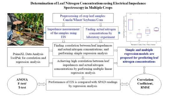
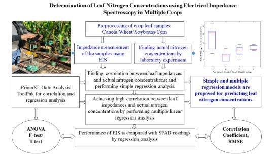
Therefore, the objectives of this study are the following: (i) To find the correlations between leaf nitrogen concentrations and leaf impedances of canola, wheat, soybeans, and corn, using simple and multiple regression analysis; (ii) to predict or determine the leaf nitrogen concentrations of the four different plant species using EIS with the help of multiple regression analysis; and (iii) to compare the performance of EIS with the SPAD measurement for the determination of leaf nitrogen concentrations.
2. Materials and Methods
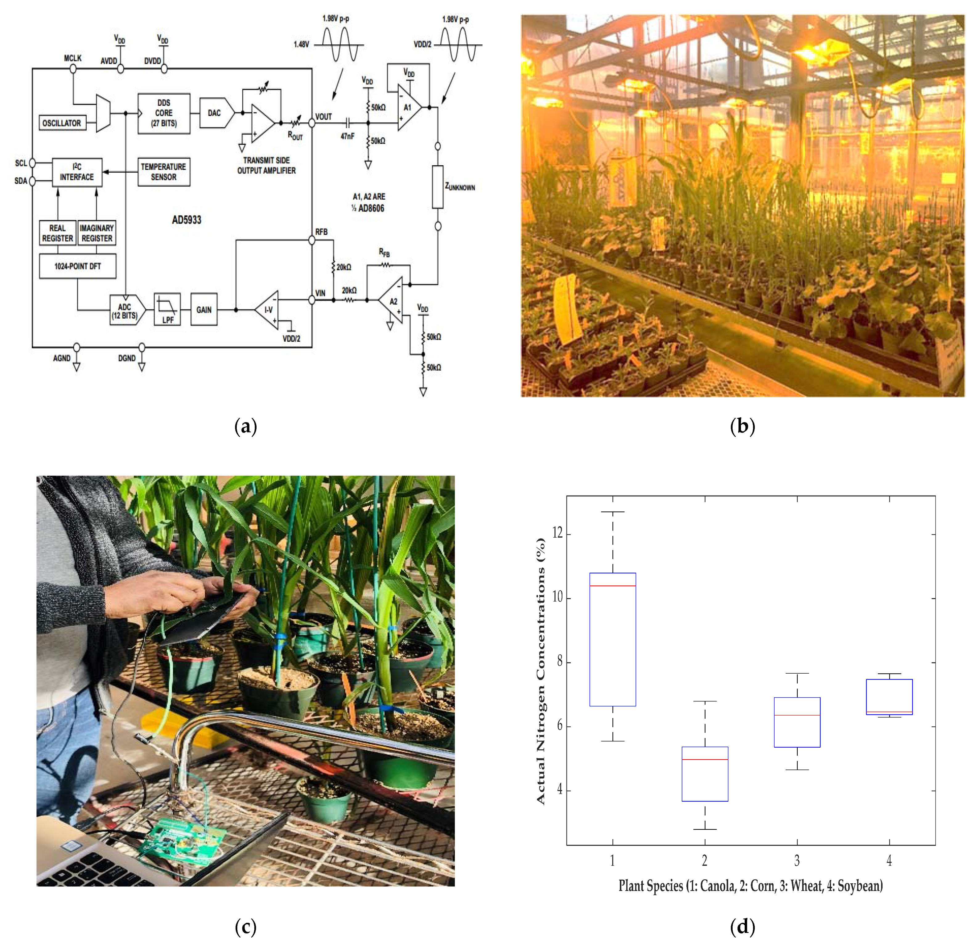
The EVAL-AD5933EBZ evaluation board (Analog Devices Inc.) is a high-precision impedance converter system that combines an on-board frequency generator with a 12-bit, 1 mega sample per second (MSPS) analog-to-digital converter (ADC), and an internal temperature sensor. The schematic diagram of the board is shown in
Figure 1a [
28]. Both the excitation signal and response signal are sampled by the ADC. The frequency range of the board is from 5 to 100 kHz without external components. Frequencies lower than 5 kHz are achievable using an external divider. The device has a master clock of 16.77 MHz. Although the device is model dependent, it offers high accuracy and versatility for a well-fitted model, which makes it suitable for electrochemical analysis, corrosion monitoring, automotive sensors, proximity sensing, and bio-impedance measurements.
The experiments were carried out at the greenhouse of the Agriculture and Agri-Food Canada (AAFC), Research and Development Centre, Saskatoon, Saskatchewan, Canada, as shown in
Figure 1b. The experimental setup of the EIS data acquisition system, as shown in
Figure 1c, was connected to a graphical user interface of the supporting software. For impedance spectroscopy measurements, a 2V
p-p generator voltage was used. The AC signal injected into the sample was generated by a built-in function generator of the evaluation board. The frequency generator allows an external complex impedance to be excited with a known frequency. This portable impedance converter network analyzer was used in EIS for measuring the impedances of the four different plant leaves (e.g., canola, wheat, soybeans, and corn) by varying the frequency in a range of 5 to 15 kHz. A pair of electrodes for an electrocardiogram (ECG) were connected to the evaluation board and used to measure the impedance of the leaf samples noninvasively. A separation of 3 cm between the two electrodes was maintained for all the measurements. Although the EIS method is time-consuming for large crops, the test duration is short because of on-board implementation which enables measurements at particular frequencies.
The leaf impedance measurement was done on a selected number of observations or samples (n) of the four different plant species. The plants were fertilized with different nitrogen levels of 0, 6, 12, and 20 g/liter with a constant water regime. A total of 111 samples were selected as follows: canola 26, wheat 36, soybeans 21, and corn 28. The experiments were carried out with the available number of samples of each plant species at the AAFC greenhouse 5 to 6 weeks after sowing. The measurements were performed in the vegetative growth stage of the crops. The impedance (Z) of a leaf sample was measured at 100 Hz intervals within the 5 to 15 kHz frequency range. A total of 101 features (k) were selected at different frequency points: f1 (5.1 kHz), f2 (5.2 kHz), f3 (5.3 kHz), …, f101 (15 kHz). The impedance at each frequency point is considered a feature. Therefore, the whole dataset of a particular plant species consisted of 101 features for the given samples.
The impedance is related to the gain factor as follows:
The magnitude of the impedance can be calculated as
where
R is the resistance and
X is the reactance, and the gain factor is determined by the calibration using a known resistance of 7.5 kΩ [
31].
After the impedances were measured, the samples with nitrogen concentrations were dried in a 60 °C incubator for 2 days. Then, the dry samples were weighted and made into powder. The actual percentages of nitrogen concentration (i.e., (nitrogen mg/mass) × 100) were measured from the powdered samples with the help of laboratory experiments using a LECO TruMac nitrogen analyzer, where nitrogen mg = ((area × calibration) − blank) × drift × sensitivity factor. The obtained results for the different plant species are represented by the boxplots, as shown in
Figure 1d. It was determined that the nitrogen concentrations are different in the different plant species. The size and area of the leaf samples vary with the different plant species, as well as their physiological properties. In the example, as shown in
Figure 1d, canola has high nitrogen concentrations as compared with the other plant species.
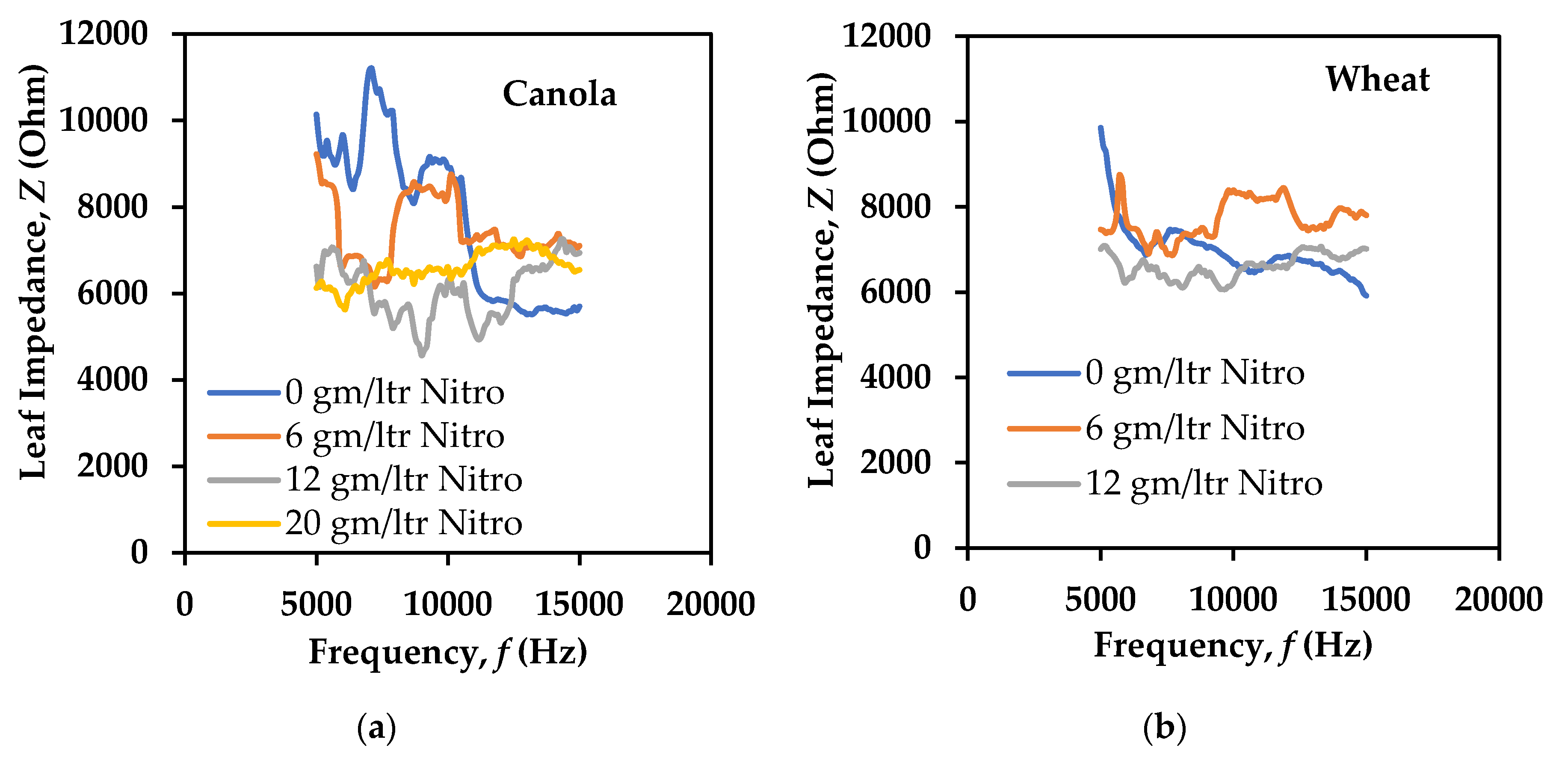
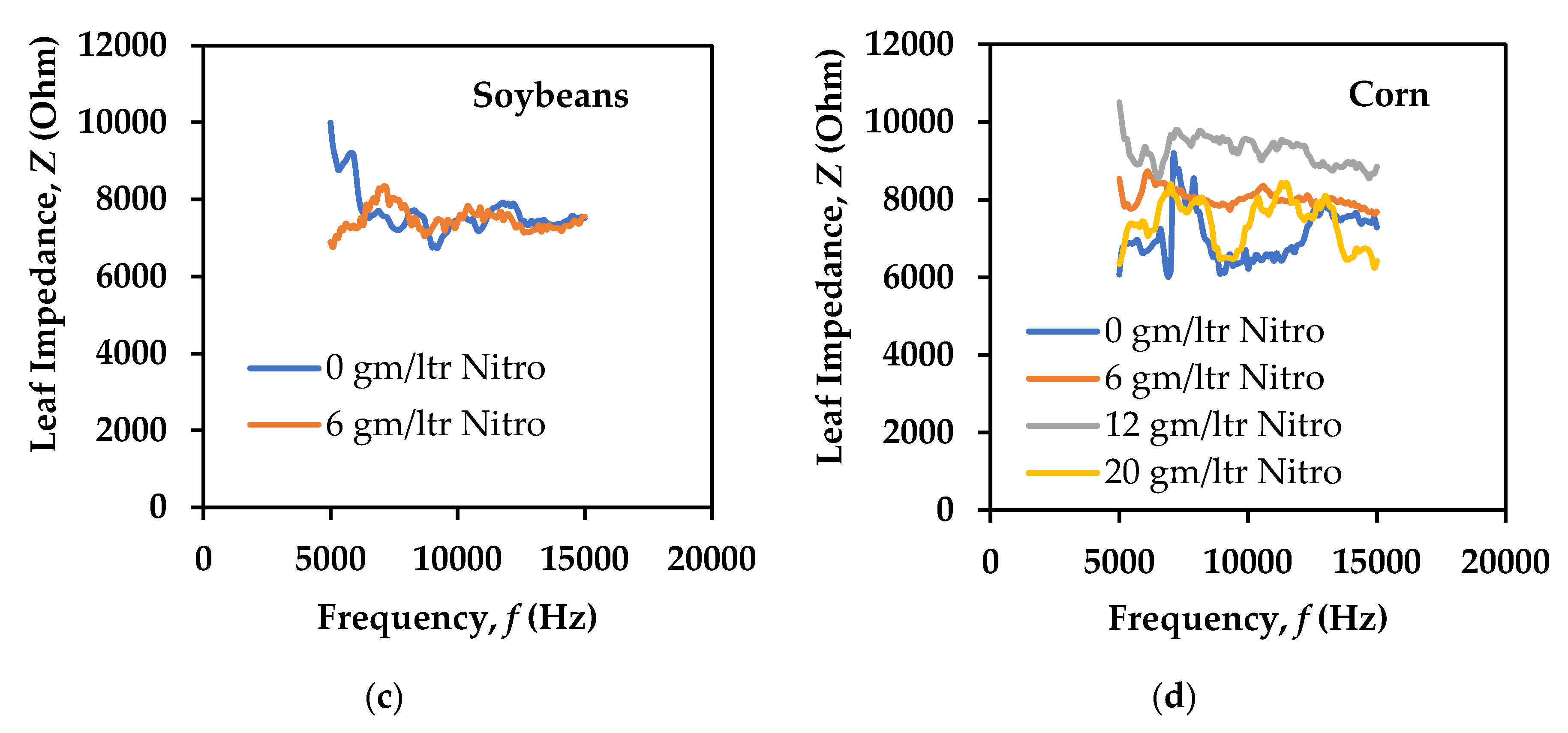
The examination of two or three leaf samples from individual plants of each species shows the average impedance profiles of the samples at varying frequencies for different nitrogen fertilization levels (see
Figure 2). It was determined that the leaf impedance of the plants decreases with an increase of frequency. Leaf impedance also decreases with an increase of nitrogen levels in the plants. The average impedance profile varies from 6 to 10 kohm with the variation of nitrogen fertilization levels from 0 to 20 gm/liter for a frequency range of 5 to 15 kHz. A high impedance profile is obtained for canola and corn as compared with soybeans and wheat. The measured impedances were examined to obtain correlations with the leaf nitrogen concentrations.
In this work, simple and multiple linear regressions using the least square method were applied to determine any correlations between plant leaf nitrogen concentrations and leaf impedances. The results were obtained by XLMiner and PrimaXL Analysis ToolPaks and validated by analysis of variance (ANOVA) tests. In multiple regression, the number of features was considered along with the observations in a given frequency range. In order to obtain optimized regression models, either the feature selection or dimensionality reduction (DR) method can be applied to reduce the number of features in a dataset. The feature selection method using backward elimination was selected and applied in this work. For different observations of the plant species, the nitrogen concentrations are predicted accordingly. The correlation coefficient (R) between leaf impedance and nitrogen concentration was determined. The corresponding coefficient of determination (R2), adjusted R2, and root mean square error (RMSE) were also determined along with the ANOVA F-test and T-test, using multiple linear regression. In this work, the training and tests were performed with the same dataset, using statistical analysis. After taking the whole dataset, the features within the highest p-value (i.e., greater than 0.05) were removed. The prediction was confirmed for all the trained datasets by the obtained p-values less than or equal to 0.05 in both the F-test and T-test. After a few iterations, the multiple regression models were obtained for the selected features of different crops.
3. Results
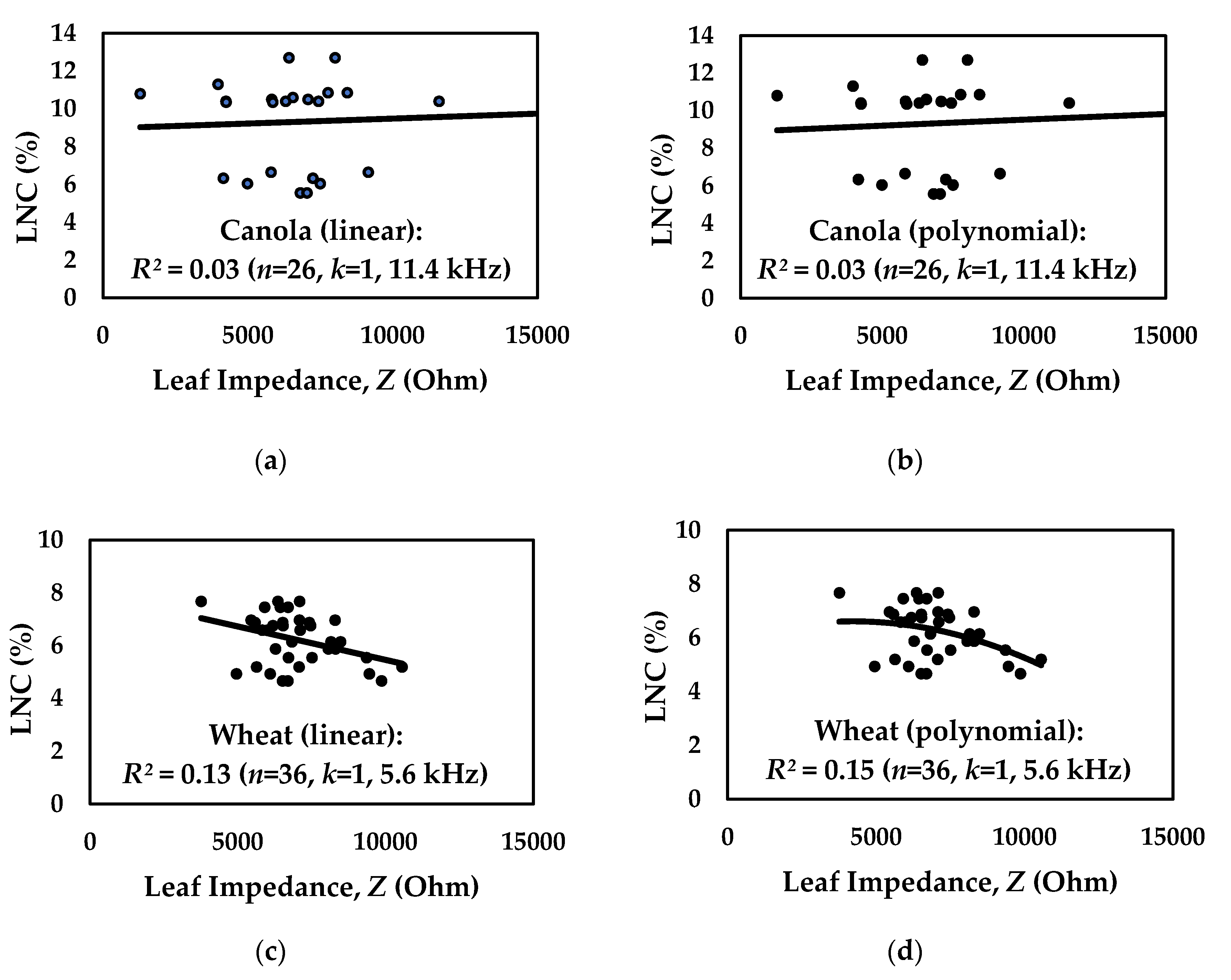
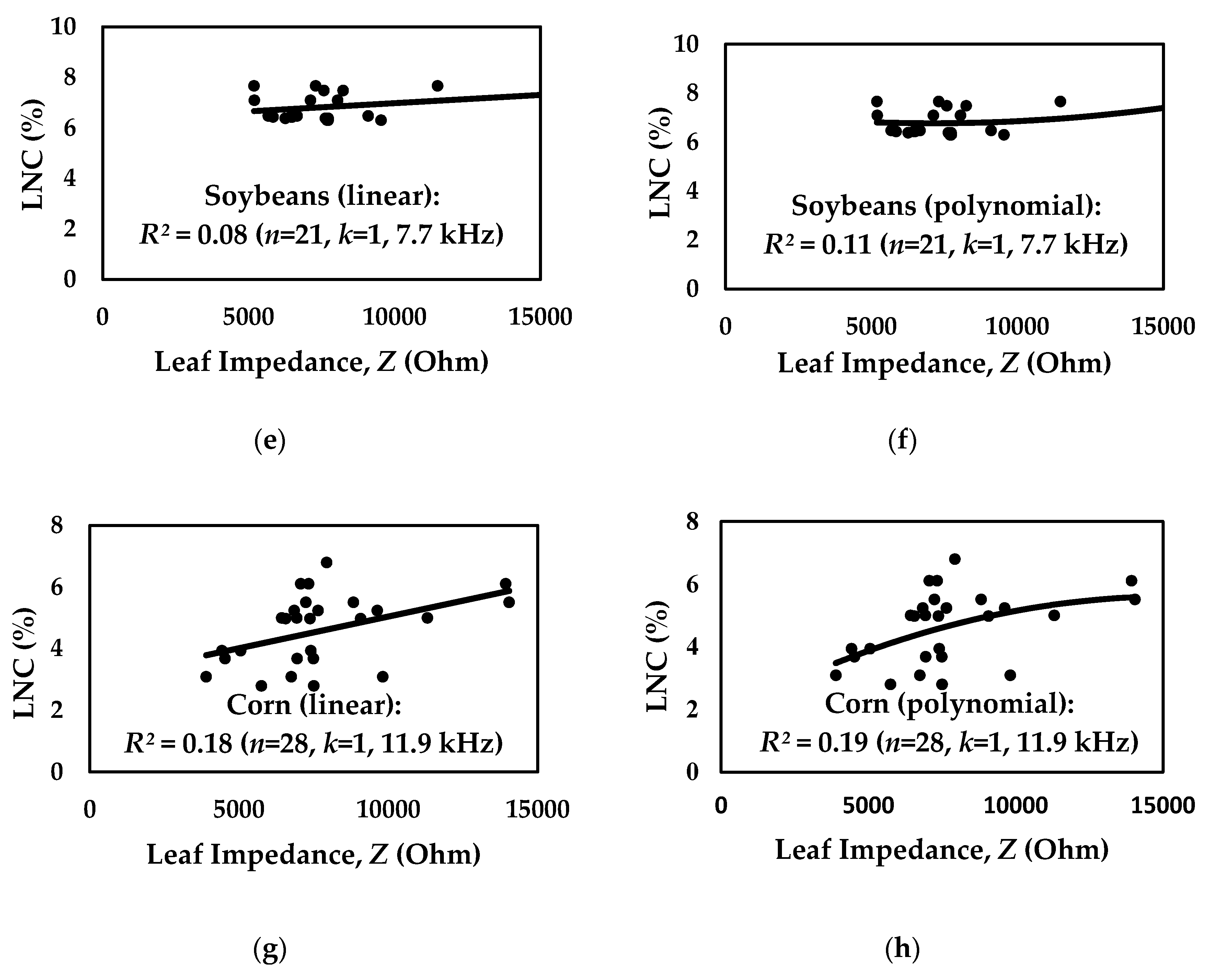
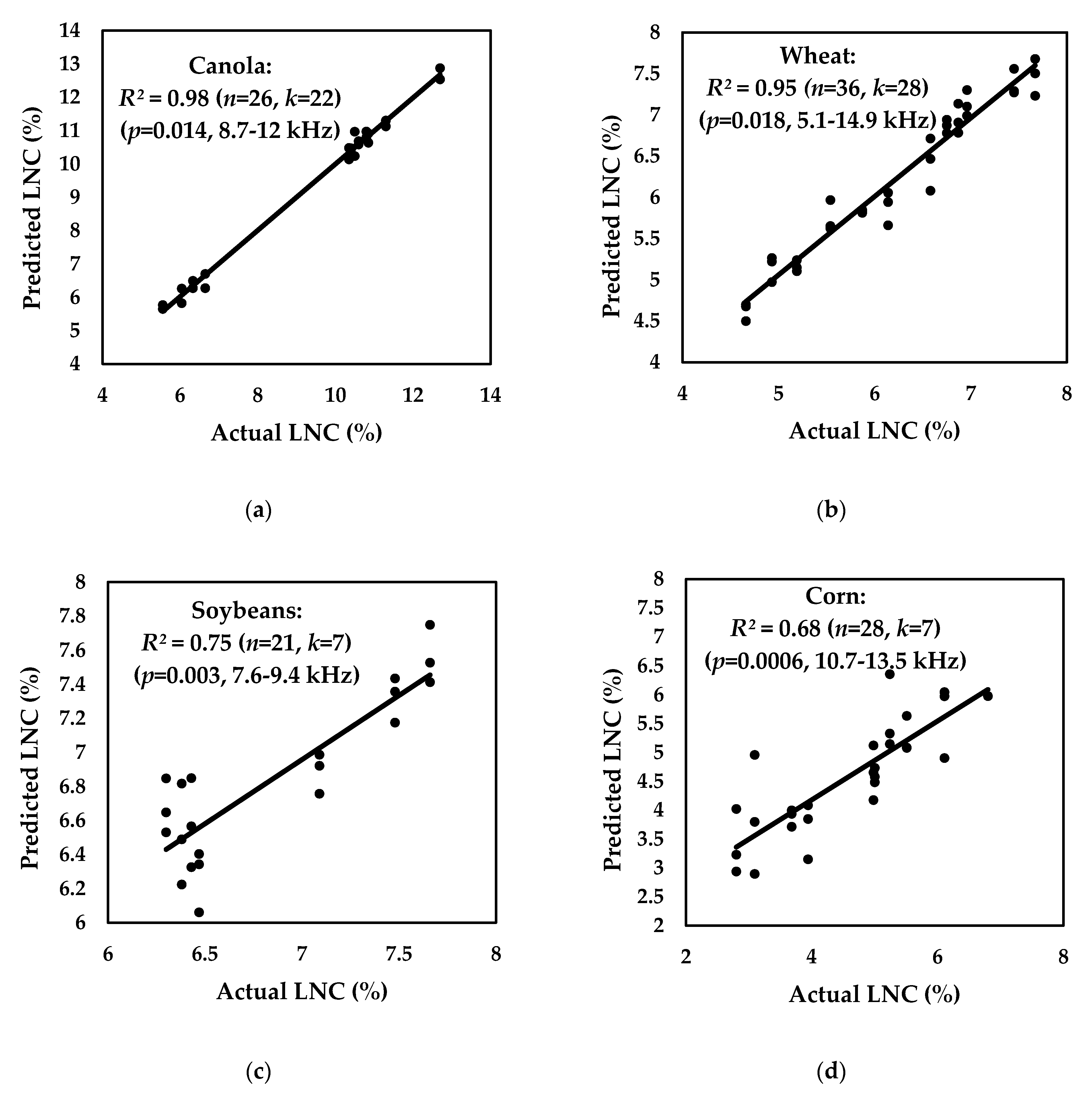
First, with the use of simple regression analysis, the maximum correlations between leaf impedance (
Z) and LNC for a single feature were found for canola, wheat, soybeans, and corn, as shown in
Figure 3. A positive correlation for canola was obtained at 11.4 kHz, a negative correlation for wheat at 5.6 kHz, a positive correlation for soybeans at 7.7 kHz, and a positive correlation for corn at 11.9 kHz. The results are shown in
Table 1.
Linear and polynomial (order 2) curve fitting methods and simple regression models were used for the different plant species at the highest correlation point. A better correlation was found for polynomial curve fitting as compared with linear in different frequencies of simple regression of the plant species. A maximum correlation coefficient (R) of 0.44 was obtained for corn, 0.39 for wheat, 0.34 for soybeans, and 0.19 for canola. On the one hand, based on a single feature, a moderate correlation was found for corn and wheat, on the other hand, the correlation was weak for soybeans and canola. Overall, the correlation results for different plant species are not satisfactory with simple regression analysis.
Next, multiple regression analysis was used to obtain better correlation results. Principal component analysis (PCA) is a popular dimensionality reduction (DR) approach of multiple regression and mostly applicable in hyperspectral image analysis, but it works extremely well for variables that are strongly correlated [
32]. PCA is very useful in data analysis using machine learning. Since the correlations are poor between the variables, according to the above results of simple regression analysis, PCA would not perform well to reduce the features in a dataset. Hence, the feature selection approach using the backward elimination method was tried in order to obtain a good correlation with multiple regression. Initially, the number of features was selected from all the features, based on the number of observations (
n) and number of features (
k =
n − 2), from the best correlation results obtained and validated by XLMiner Analysis ToolPak. For the given observations, the number of features was selected accordingly, using the standard backward elimination method to obtain the best correlation and regression results. The importance of the features was checked sequentially with the help of ANOVA F/T tests for obtaining the best multiple regression model. An optimization was done, and the best multiple regression results for the different plant species with nitrogen concentrations are summarized in the following section.
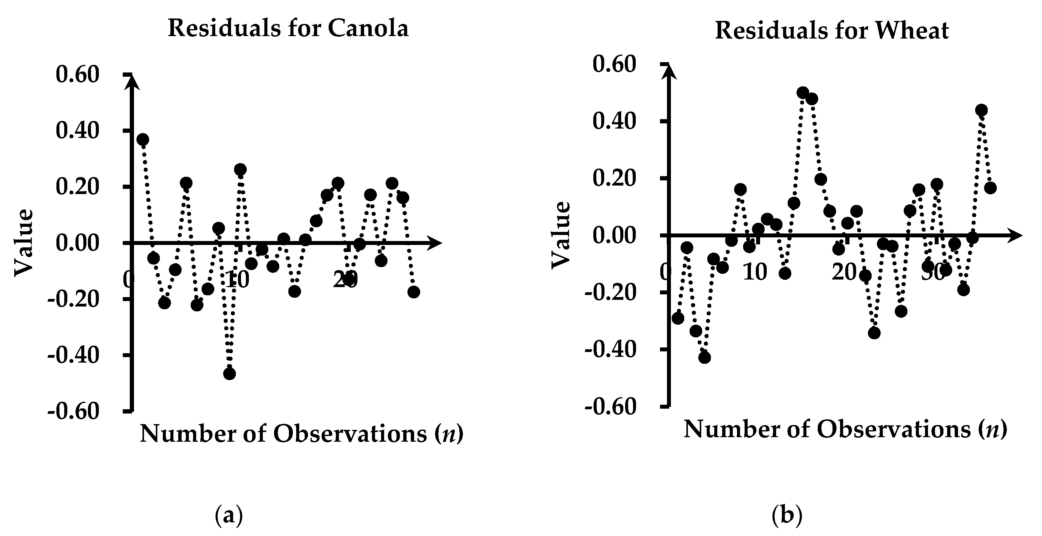
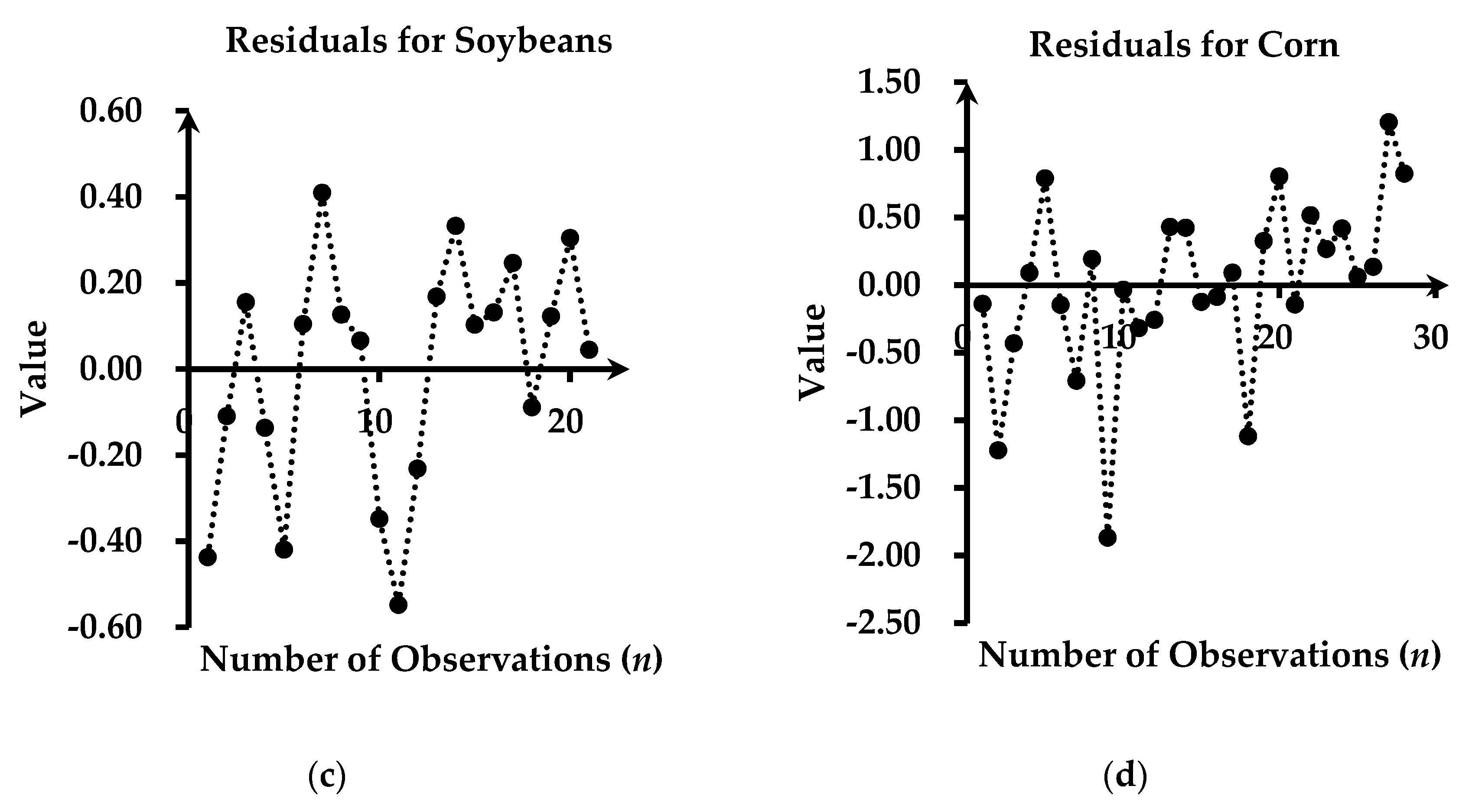
With multiple regression analysis, employing the least square method, the residuals were obtained for multiple observations with selected features using Residual value = actual value − predicted value. A random pattern of residuals supports a linear model. The sum of the residuals is always zero, whether the dataset is linear or nonlinear. The residuals for different observations and the corresponding best regression line between actual versus predicted nitrogen concentrations for the four different plant species are presented in
Figure 4 and
Figure 5, respectively.
The coefficient of determination is calculated using the following:
The adjusted
R2 is calculated as
and the root mean square error (RMSE) is calculated as follows:
Here,
where
y is the actual LNC obtained by the experiment of laboratory measurement,
is the mean value of the actual LNC, and
is the predicted LNC obtained by multiple regression analysis using the least square method [
33,
34,
35,
36].
The predicted leaf nitrogen concentrations were validated by comparison with the actual leaf nitrogen concentrations. The overall multiple linear regression analysis results for different plant species are shown in
Table 2. Overall, high correlation results were obtained using multiple regression analysis. The number of features was further reduced to avoid overfitting, and the regression results for different plant species are also included in
Table 2. It was found that the correlation coefficient, the coefficient of determination, and adjusted
R2 decreased with the decrease of the features, and that the corresponding RMSE increased. The feature selection was done by positive ANOVA tests using
p-value less than or equal to 0.05.
A maximum correlation coefficient of 0.99 is obtained for canola, using multiple features ranging from 8.7 to 12 kHz. The maximum coefficient of determination for canola is 0.98, the adjusted
R2 is 0.94, RMSE is 0.54%, and the ANOVA tests are positive; here,
SSR = 133.58,
SSE = 0.87,
SST = 134.46, and
p-value = 0.014 (F-test). From 101 features, only 22 were selected to obtain the best correlation and regression results using ANOVA tests. Overfitting was reduced by the backward elimination of features with
p-values greater than the threshold. The chances of overfitting could also be reduced by minimizing the features to 10 or nine, which would also reduce the corresponding correlation coefficient to 0.85 or 0.78, respectively. On the basis of the maximum correlation, the proposed model for the predicted nitrogen concentrations in canola for multiple features is extracted as:
where the 11th feature of 10.9 kHz, 13th feature of 11.1 kHz, 14th feature of 11.2 kHz, and the 20th feature of 11.8 kHz with
p-values of 0.014, 0.02, 0.02, and 0.027, respectively, in the T-test contributed less to the model than the other features.
A maximum correlation coefficient of 0.97 is obtained for wheat, using multiple features ranging from 5.1 to 14.9 kHz. The maximum coefficient of determination for wheat is 0.95, the adjusted
R2 is 0.75, RMSE is 0.47%, and the ANOVA tests are positive; here,
SSR = 30.67,
SSE = 1.56,
SST = 32.23, and
p-value = 0.018 (F-test). From 101 features, only 28 were selected to obtain the best correlation and regression results using ANOVA tests. Overfitting was reduced by the backward elimination of features with
p-values greater than the threshold. The chances of overfitting could also be reduced by minimizing the features to 17 or 11, which would also reduce the corresponding correlation coefficient to 0.86 or 0.75, respectively. On the basis of maximum correlation, the proposed model for the predicted nitrogen concentrations in wheat for multiple features is extracted as:
where the 2nd feature of 5.2 kHz, 7th feature of 5.8 kHz, 9th feature of 6.1 kHz, 14th feature of 7.2 kHz, 15th feature of 7.4 kHz, 17th feature of 7.6 kHz, 21st feature of 8 kHz, 24th feature of 8.3 kHz, and the 26th feature of 8.9 kHz with
p-values of 0.021, 0.011, 0.024, 0.01, 0.015, 0.041, 0.028, 0.013, and 0.016, respectively, in the T-test contributed less to the model than the other features.
A maximum correlation coefficient of 0.86 is obtained for soybeans, using multiple features ranging from 7.6 to 9.4 kHz. The maximum coefficient of determination for soybeans is 0.75, the adjusted
R2 is 0.62, RMSE is 0.33%, and the ANOVA tests are positive; here,
SSR = 4.41,
SSE = 1.44,
SST = 5.85, and
p-value = 0.003 (F-test). From 101 features, only seven were selected to obtain the best correlation and regression results using ANOVA tests. Overfitting was reduced by the backward elimination of features with
p-values greater than the threshold. The chances of overfitting could also be reduced by minimizing the features to five or four, which would also reduce the corresponding correlation coefficient to 0.75 or 0.70, respectively. On the basis of the maximum correlation, the proposed model for the predicted nitrogen concentrations in soybeans for multiple features is extracted as:
where the 3rd feature of 8.6 kHz with a
p-value of 0.033 in the T-test contributed less to the model than the other features.
A maximum correlation coefficient of 0.82 is obtained for corn, using multiple features ranging from 10.7 to 13.5 kHz. The maximum coefficient of determination for corn is 0.68, the adjusted
R2 is 0.57, RMSE is 0.76%, and the ANOVA tests are positive; here,
SSR = 25.04,
SSE = 11.63,
SST = 36.68, and
p-value = 0.0006 (F-test). From 101 features, only seven were selected to obtain the best correlation and regression results using ANOVA tests. Overfitting was reduced by the backward elimination of features with
p-values greater than the threshold. The chances of overfitting could also be reduced by minimizing the features to four or three, which would also reduce the corresponding correlation coefficient to 0.73 or 0.64, respectively. On the basis of the maximum correlation, the proposed model for the predicted nitrogen concentrations in corn for multiple features is extracted as:
where the 1st feature of 10.7 kHz and the 6th feature of 13.1 kHz with
p-values of 0.037 and 0.027, respectively, in the T-test contributed less to the model than the other features.
The proposed models using EIS are accurate and global for the individual plant species only. For each crop, different features were selected in the model based on the positive ANOVA tests because of different physiological properties. For canola and wheat, the individual features contribute less to the correlation, and thus a higher number of features are required as compared with soybeans and corn. The computation is complex in EIS and it is model dependent. For different plant species, datasets are different, and different models are required for the estimation. Appropriate fitting of the models shows the accuracy of the measurement using an EIS board.
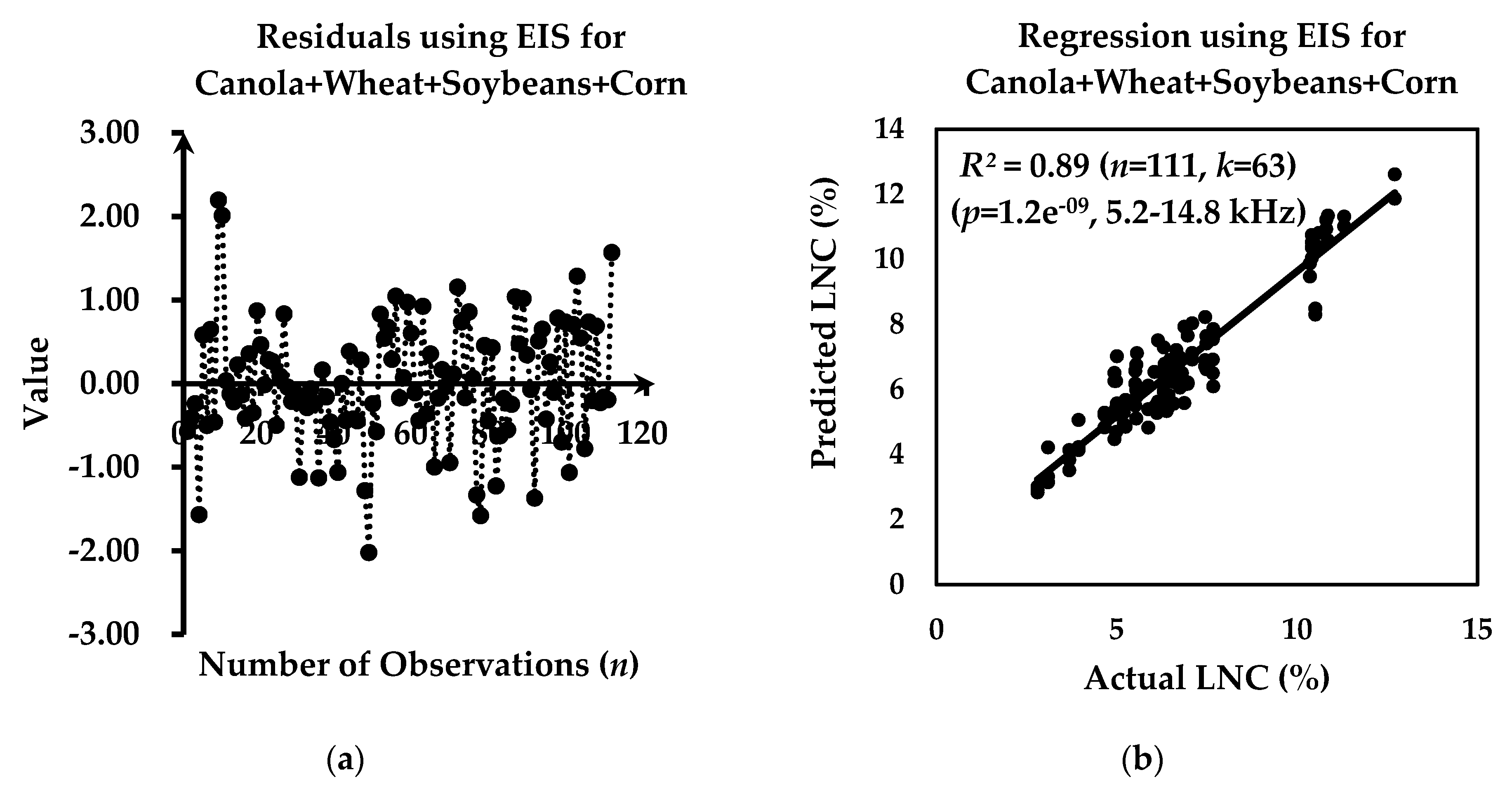
Next, all the observations of different plant species were combined, and the multiple regression analysis was done using PrimaXL Analysis ToolPak. For multiple regression, a linear regression line was found between actual leaf nitrogen concentration and the predicted leaf nitrogen concentration for canola + wheat + soybeans + corn, using EIS, as shown in
Figure 6. The coefficient of determination is 0.89 and the overall correlation coefficient is 0.94.
The SPAD leaf chlorophyll meter is a handheld, self-calibrating, and convenient device for a rapid and nondestructive assessment of leaf chlorophyll content in different crops. The leaf chlorophyll content is correlated to the leaf nitrogen concentration depending on the variety of plant species, locations, and growth stages [
9,
10,
37]. For this, the measurement of leaf nitrogen concentration is possible using SPAD, and the relationship is curvilinear. SPAD measures the transmittance of red (650 nm) and infrared (940 nm) radiation through the leaf using two silicon photodiode detectors and has gained in popularity for its ease of use, although it is not as accurate as the destructive method. It utilizes the light attenuation difference between these two wavelengths to determine leaf greenness. Green color intensity of a crop leaf is directly related to the leaf nitrogen concentration and depending on the position of measurement on a leaf surface and area of the leaf, SPAD can have utility in predicting leaf nitrogen concentration [
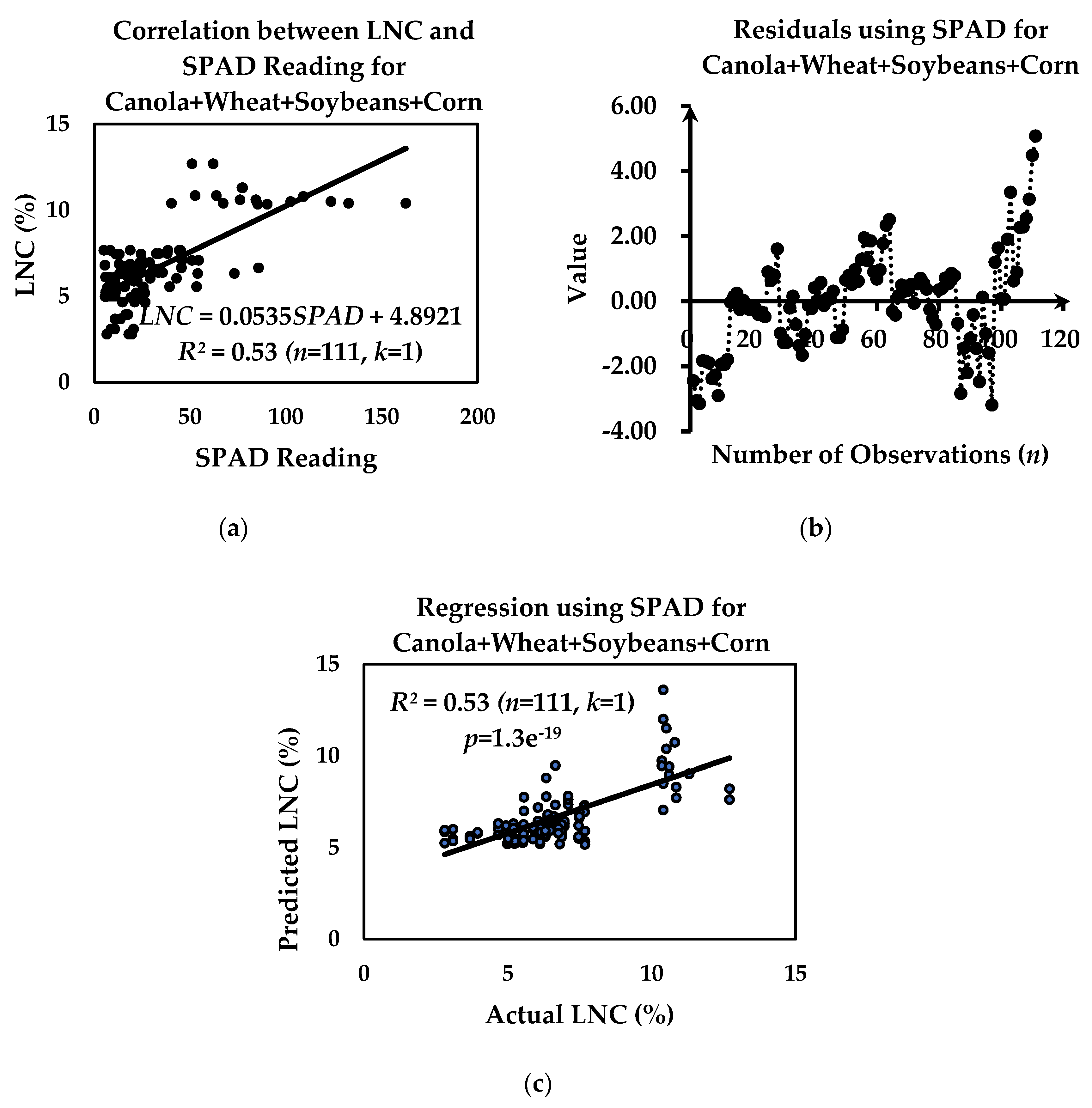
37]. For the combined observations, the performance of EIS as compared with SPAD readings is presented in
Figure 7, and the summarized results are shown in
Table 3.
Using EIS, an overall maximum correlation coefficient of 0.94 and a coefficient of determination of 0.89 are obtained for the combined 111 observations of the plant species with nitrogen concentrations, where 63 features from 5.2 to 14.8 kHz were selected, and the RMSE is 1.12%. Overfitting is reduced by the backward elimination of features with p-values greater than the threshold. The chances of overfitting could also be reduced by minimizing the features from 63 to 33, which would also reduce the maximum correlation coefficient to 0.81. However, for the same number of observations using SPAD, a maximum correlation coefficient of 0.72 is obtained, where the coefficient of determination is 0.53 and the RMSE is 1.52%. Thus, EIS performs well as a good alternative to optical spectroscopy and to other nondestructive methods, such as SPAD, for the determination of leaf nitrogen concentrations.
4. Summary and Discussion
In EIS measurement, it was determined that impedance varies with the variation of frequency for the four different crop leaves. The leaf impedance decreases with an increase of frequency and also with an increase of the nitrogen fertilization level. The actual nitrogen concentrations in the leaves were measured by a nitrogen analyzer, the samples were trained, and the nitrogen concentrations for all of them were predicted by regression analysis.
The correlation between actual nitrogen concentrations and the measured impedances of the leaves was found with simple regression analysis, but the obtained correlation with a single feature was not satisfactory. Therefore, multiple linear regression was also utilized to obtain better correlation results with the help of PrimaXL Toolpak. The selection of the number of features was challenging, but, along with the observations, played an important role in regression analysis. Removal of features using backward elimination had to be done very carefully, otherwise, the wrong selection may have affected the correlation and regression results. The overall correlation coefficient (R), coefficient of determination (R2) and its adjusted value, and RMSE were calculated for the four different crops using Equations (3) to (8). After various experiments, it was found that the correlation coefficient and the coefficient of determination increased with an increase in the number of features for a given number of observations, and the corresponding RMSE decreased. The optimized selected features create a suitable model for good predictions.
The residuals were obtained from the difference between actual and predicted nitrogen concentrations. The lower residuals helped to achieve a good regression model for different observations. Multiple linear regression results, presented in
Table 2, show that the highest correlation coefficient of 0.99 is obtained for canola, while 0.97 is obtained for wheat, 0.86 for soybeans, and 0.82 for corn. The corresponding RMSE values are 0.54%, 0.47%, 0.33%, and 0.76%, respectively. After training, the predicted results were tested and validated with the resulting positive ANOVA F-test and T-test, using
p-values less than or equal to 0.05. The obtained results are satisfactory in comparison with previously published works [
16,
17,
18,
19]. The proposed models show that a large number of features are required for canola and wheat because the individual feature correlation is not very strong, a few features in the models contributed less to the correlation. The proposed models for soybeans and corn required a lower number of features because of strong individual feature correlation. However, a few features still contributed less to the correlation.
The performance of EIS was also compared with the SPAD measurement. A maximum correlation coefficient of 0.94 is obtained with a minimum RMSE of 1.12%, using EIS measurements for 111 observations, whereas, for the same observations and using SPAD, a maximum correlation coefficient of 0.72 is obtained, and the RMSE is 1.52%. Overall, satisfactory results are presented in this work in comparison with previously published works on optical spectroscopy [
4], [
7], and on electrical impedance spectroscopy [
21,
22]. A strong correlation was found between nitrogen concentrations and impedances of the crop leaves measured by EIS with multiple features, and the nitrogen concentrations of the leaves were also determined accurately with the best multiple regression results.


