Article

Modelling Global Ionosphere Based on Multi-Frequency, Multi-Constellation GNSS Observations and IRI Model

1
GNSS Research Center, Wuhan University, 129 Luoyu Road, Wuhan 430079, China
2
Nottingham Geospatial Institute, The University of Nottingham, Nottingham NG7 2TU, UK
3
School of Geodesy and Geomatics, Wuhan University, 129 Luoyu Road, Wuhan 430079, China
4
Key Laboratory of Geospace Environment and Geodesy, Ministry of Education, Wuhan University, 129 Luoyu Road, Wuhan 430079, China
*
Author to whom correspondence should be addressed.
Remote Sens. 2020, 12(3), 439; https://doi.org/10.3390/rs12030439
Submission received: 2 January 2020 / Revised: 29 January 2020 / Accepted: 30 January 2020 / Published: 31 January 2020

Abstract

:
With the emergence of BeiDou and Galileo as well as the modernization of GPS and GLONASS, more available satellites and signals enhance the capability of Global Navigation Satellite Systems (GNSS) to monitor the ionosphere. However, currently the International GNSS Service (IGS) Ionosphere Associate Analysis Centers (IAACs) just use GPS and GLONASS dual-frequency observations in ionosphere estimation. To better determine the global ionosphere, we used multi-frequency, multi-constellation GNSS observations and a priori International Reference Ionosphere (IRI) to model the ionosphere. The newly estimated ionosphere was represented by a spherical harmonic expansion function with degree and order of 15 in a solar-geomagnetic frame. By collecting more than 300 stations with a global distribution, we processed and analysed two years of data. The estimated ionospheric results were compared with those of IAACs, and the averaged Root Mean Squares (RMS) of Total Electron Content (TEC) differences for different solutions did not exceed 3 TEC Unit (TECU). Through validation by satellite altimetry, it was suggested that the newly established ionosphere had a higher precision than the IGS products. Moreover, compared with IGS ionospheric products, the newly established ionosphere showed a more accurate response to the ionosphere disturbances during the geomagnetic storms.

Graphical Abstract

1. Introduction

The ionosphere constitutes the upper part of the atmosphere, extending from approximately 60 to 1500 km above the Earth’s surface, enriched with free electrons and ions. It is a particularly important region with regard to radio signal propagation and radio communications in general. The ionosphere is dispersive, which means that the time delay attributed to the ionosphere depends on the frequency of the signal. This dispersive property also makes the multi-frequency Global Navigation Satellite Systems (GNSS) efficiently sense the ionospheric activities and ionisation [1,2,3]. In the meantime, with the modernization of GPS and GLONASS as well as the rapid deployments of BeiDou System (BDS) and Galileo, more and more satellites are available to transmit multi-frequency signals, which brings both opportunities and challenges for ionosphere monitoring and modelling.
The International GNSS Service (IGS) Ionosphere Working Group was initialized in 1998 to exploit the global ionosphere estimation based on the IGS network of stations, and routinely provides IGS Global Ionosphere Maps (GIMs) based on a weighted combination of ionosphere maps regularly produced by IGS Ionosphere Associate Analysis Centers (IAACs) [4], such as the Center for Orbit Determination in Europe (CODE), European Space Agency (ESA), Jet Propulsion Laboratory (JPL) and Polytechnic University of Catalonia (UPC). IAACs employ different data sets and methods to model the GIMs. CODE and ESA collect data from about 280 globally distributed GPS and GLONASS sites. The GIMs are determined in a solar-geomagnetic reference frame using spherical harmonic (SH) expansion in combination with a daily Differential Code Bias (DCB) estimation [5,6,7,8]. JPL and UPC just use GPS data to estimate the GIMs. The Total Electron Content (TEC) is modelled in a solar-geomagnetic reference frame using bi-cubic splines on a spherical grid in JPL. Whilst for UPC, the GIMs are modelled independently for each station with a tomographic model: cells in local time, latitude and height [9].
Currently, BDS and Galileo are playing a more and more important role in ionosphere determination. BDS had 21 Medium Earth Orbit (MEO), 9 Inclined Geo-Synchronous Orbit (IGSO) and 5 Geostationary Earth Orbit (GEO) satellites in normal operation by January 2020, while Galileo had 22 usable satellites. With the increase of in-orbit BDS and Galileo satellites, a better satellite distribution will be achieved and hence the ionosphere pierce points will be remarkably increased. The additional measurements from BDS and Galileo will be helpful to model the ionosphere more precisely [10,11,12]. The advantage of combined ionosphere determination with dual-frequency measurements from GPS, GLONASS, BDS and Galileo has also been assessed through a 60-day performance analysis by Ren et al. [13].
The increased frequencies and satellites undoubtedly benefit the global ionosphere determination. However, previous contributions mainly use GPS and GLONASS observations to model the global ionosphere. Even for the ionosphere estimation based on quad-constellation GNSS, only the traditional dual-frequency measurements are used. Therefore, the potential capacity of multi-frequency and multi-constellation GNSS in ionosphere modelling needs to be fully explored. Although sensing the global ionosphere by GNSS has many advantages, its performance depends on the distribution of the data source. Especially for the region with limited data, the ionosphere model is relatively weak. Then, the advanced International Reference Ionosphere (IRI) model [14,15,16] is introduced as an a priori ionosphere to make the ionospheric model stronger.
To attain a meaningful conclusion, we processed the long-term data of 2017 and 2018. With a priori IRI model, the ionospheric improvements brought by multi-frequency and multi-constellation GNSS were compared with the solutions from other IAACs and independently validated by satellite altimetry [4,17]. The ionospheric accuracy and performance during two geomagnetic storms in the two years were especially comprehensively analysed. Section 2 describes the mathematical model of the global ionosphere estimation; the stations used in the manuscript are shown in Section 3, and followed by the results and analysis; the conclusions are given in the final section.

2. Mathematical Model

Extracting absolute TEC information from multi-frequency GNSS observations is a prerequisite for ionosphere estimation and is firstly introduced, followed by the derivation of the initial ionospheric information from the IRI model. Then, the method of global ionosphere representation is described. Finally, we generated GIMs and Root Mean Square (RMS) maps in Ionosphere Exchange (IONEX) format [18].

2.1. Ionospheric Observation Equation

The unambiguous GNSS code measurements are widely used in ionosphere estimation. To significantly reduce the noise of code measurements, the so-called “phase-smoothed code” algorithm is used based on a continuous time series of code and phase measurements [5]. Assuming a common “cycle-slip-free” period of n epochs, the smoothed code measurements from receiver a to satellite i at epoch t are written as:
{ P ˜ a , 1 i ( t ) = P ¯ a , 1 i + Δ L a , 1 i ( t ) + 2 f m 2 f 1 2 f m 2 ( Δ L a , 1 i ( t ) Δ L a , m i ( t ) ) P ˜ a , m i ( t ) = P ¯ a , m i + Δ L a , m i ( t ) + 2 f 1 2 f 1 2 f m 2 ( Δ L a , 1 i ( t ) Δ L a , m i ( t ) )
where
{ Δ L a , 1 i ( t ) = L a , 1 i ( t ) L ¯ a , 1 i Δ L a , m i ( t ) = L a , m i ( t ) L ¯ a , m i
m denotes another frequency index except for the reference frequency index 1, f is the carrier frequency (Hz), P ( t ) and L ( t ) are the raw code and phase measurements (m) at epoch t , P ¯ and L ¯ denotes the averaged code and phase measurements (m) over the n epochs.
The undifferenced observation equations of smoothed code measurements at epoch t can be reformulated as follows:
{ P ˜ a , 1 i ( t ) = ρ a i + c ( d t i d t a ) + T a i + 40.3 E a i f 1 2 + δ h 1 i δ b a , 1 + ε P ˜ a , m i ( t ) = ρ a i + c ( d t i d t a ) + T a i + 40.3 E a i f m 2 + δ h m i δ b a , m + ε
where ρ means the geometric distance between the antennas of receiver and satellite (m); c is the speed of light in vacuum (m/s); d t i and d t a represents the satellite and receiver clock bias (s); T depicts tropospheric delay (m); E is the Slant TEC (STEC) in the signal propagation path in unit of TEC Unit ( 1   TECU   =   10 16 el / m 2 ); δ h and δ b are the hardware biases of satellite and receiver (m). A priori noise of the unsmoothed raw code measurement is set as 0.6 m, ε is the observation noise of the smoothed code measurement (m), which is reduced by about a factor of n with respect to the a priori noise.
The ionospheric observation can be obtained through differencing the smoothed measurements at different frequencies [5]:
P ˜ a , m 1 i ( t ) = P ˜ a , m i ( t ) P ˜ a , 1 i ( t ) = 40.3 ( 1 f m 2 1 f 1 2 ) E a i + δ h m 1 i δ b a , m 1 + ε i o n
where ε i o n = 2 × ε , δ h m 1 i and δ b a , m 1 denote the satellite and receiver DCB between frequencies m and 1.

2.2. Initial Ionospheric Information from the International Reference Ionosphere (IRI)

The IRI (http://irimodel.org/) is an international project sponsored by the Committee on Space Research (COSPAR) and the International Union of Radio Science (URSI), the latest version is IRI-2016 [15,16]. As an advanced empirical ionospheric model, the IRI-2016 can integrate the TEC from the ground to a selected height for a given location, time and date. A priori ionospheric information helps us to strengthen the stability and reliability of the solution, especially for the regions with less available GNSS data. Based on IRI-2016, the hourly GIM was pre-generated with a spatial resolution of 5 × 2.5 in longitude and latitude. The a priori ionospheric value for each grid is seen as a pseudo-observation and inserted into the normal equation. The pseudo-observation at a grid is formatted as:
E I R I ( B , L ) = V T E C I R I ( B , L ) + ε ( E I R I )
in which B , L denote the latitude and longitude of the grid, V T E C I R I is the corresponding Vertical TEC (VTEC) derived from IRI-2016, ε ( E I R I ) represents the a priori precision of the VTEC. The precision of VTEC derived from the IRI model is around 2~5 TECU in medium and high latitudes and 5~10 TECU in low latitudes, which was deeply analyzed and well validated by various authors [19,20,21]. To avoid the absolute VTEC estimation, a relatively loose constraint of 10 TECU was employed for the region of latitudes lower than 25° and 5 TECU for the region of latitudes higher than 25°.

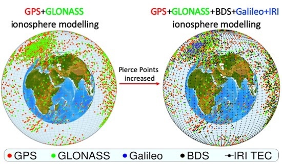
2.3. Global Ionospheric Representation

The single-layer model at an altitude of 450 km and SH expansion function are well suited to represent the global VTEC [21,22]. The VTEC was parameterised as:
E v ( β , s ) = n = 0 n max m = 0 n N n m P n m ( sin β ) ( C ˜ n m cos ( m s ) + S ˜ n m sin ( m s ) )
where E v is the VTEC (TECU); β and s denote the sun-fixed geomagnetic latitude and longitude of the ionospheric pierce point (IPP); n max is the maximum degree of the SH expansion; N n m is the normalization function [23]; P n m is the classical, unnormalized Legendre function; C ˜ n m and S ˜ n m are the unknown SH coefficients.
For absolute TEC estimation using ground-based GNSS data, the TEC along the vertical direction is of main interest. To convert the STEC to VTEC, the Modified Single-Layer Model (MSLM) mapping function was employed:
F ( z ) = 1 cos z   with   sin z = R R + H sin ( α z )
where z and z are the zenith distances (i.e., the angle measured from zenith) of the satellite at the receiver and IPP, respectively. The best MSLM mapping function was achieved at the altitude H = 506.7 km and the scale factor α = 0.9782 [24], when using the mean earth radius R = 6371 km and assuming a maximum zenith distance of 80 degrees.
Substituting (6) and (7) to (4), the multi-constellation GNSS ionospheric observations for global ionosphere determination was described as:
{ P a , m 1 G , i = 40.3 ( 1 f G , m 2 1 f G , 1 2 ) F ( z a i ) E v ( β a i , s a i ) + δ h m 1 G , i δ b a , m 1 G + ε i o n G P a , n 1 R , j = 40.3 ( 1 f R , n 2 1 f R , 1 2 ) F ( z a j ) E v ( β a j , s a j ) + δ h n 1 R , j δ b a , n 1 R + ε i o n R P a , p 1 C , k = 40.3 ( 1 f C , p 2 1 f C , 1 2 ) F ( z a k ) E v ( β a k , s a k ) + δ h p 1 C , k δ b a , p 1 C + ε i o n C P a , q 1 E , l = 40.3 ( 1 f E , q 2 1 f E , 1 2 ) F ( z a l ) E v ( β a l , s a l ) + δ h q 1 E , l δ b a , q 1 E + ε i o n E
with the initial ionospheric constraints from IRI-2016 for each grid of the hourly GIM:
E I R I ( B , L ) = E v ( β , s ) + ε ( E I R I )
where B is from the latitude 87.5 to 87.5 with an interval of 2.5 ; L is from the longitude 180 to 180 with an interval of 5 ; i , j , k , l represents GPS (G), GLONASS (R), BDS (C) and Galileo (E) satellites, respectively. m , n , p , q are frequency indexes except for the reference frequency index 1, such as m = L 2 , L 5 for GPS, n = G 2 for GLONASS, p = B 2 , B 3 for BDS and q = E 5 a , E 5 b , E 5 , E 6 for Galileo. Considering the GLONSS inter-frequency bias [25] and BDS satellite-induced code bias [26], we adopted a scale factor of 1.5 for the noise of GLONASS and BDS ionospheric observations, which means ε i o n R = ε i o n C = 1.5 ε i o n and ε i o n G = ε i o n E = ε i o n . In addition, the DCB parameters of the satellite and receiver for each observation in (8) are strongly correlated, causing singularity of the normal equation. Additional constraints need to be applied to separate the DCB of the receiver and satellites. According to the processing strategy of the IAACs, we assumed that the sum of satellite DCB parameters in one day for each constellation was equal to zero:
i = 1 N G δ h m 1 G , i = 0 , j = 1 N R δ h n 1 R , j = 0 , k = 1 N C δ h p 1 C , k = 0 , l = 1 N E δ h q 1 E , l = 0
The multi-constellation GNSS ionospheric observations are lumped to a normal equation epoch by epoch. The global ionospheric parameters are modelled as piece-wise linear function with an interval of 1 h and solved by the least square adjustment. Based on the estimated SH parameters and variance-covariance matrix, the hourly GIM and RMS maps with a resolution of 5 × 2.5 in longitude and latitude were generated through (6) and stored in IONEX format.

3. Data Sources

The Multi-GNSS Experiment (MGEX) was initialized in 2013, aiming to track, collate and analyse all available GNSS signals [27,28]. By January 2020, the MGEX network had grown to more than 300 stations and a continued expansion is expected in the future. Especially in the past two years, with the rapid deployment of BDS and Galileo, the MGEX stations have significantly increased. To achieve a meaningful conclusion, we collected data from 348 IGS and MGEX stations in 2017 and 2018, as illustrated in Figure 1. All the stations were able to track GPS signals, whilst 295, 208 and 141 stations could normally receive GLONSS, Galileo and BDS signals, respectively. Although we used 348 stations in total to model the global ionosphere, the number of stations we applied for each day was around 300, which was close to the number of stations used by the IAACs.
The Positioning and Navigation Data Analysis (PANDA) platform at Wuhan University in China [29] was extended to model the global ionosphere based on multi-frequency and multi-constellation GNSS, and the data of two years were processed with this software. Moreover, to deeply analyse, comprehensively assess and independently validate our global ionosphere products, the determined GIM was compared with the VTEC from satellite altimetry mission Jason-2/3. The final data products of satellite altimetry, issued by the French Space Agency—“Centre National d’Etudes Spatiales” (CNES), were collected from the database of the Archiving, Validation and Interpretation of Satellite Oceanographic (AVISO).
To have a clear sense of the increase of IPP brought by multi-constellation GNSS, as an example, Figure 2 plots the IPP at an epoch on the day of year (DOY) 001 in 2018. The IPP are noticeably increased since the BDS and Galileo satellites are introduced. Actually, the increase in observations is far more than the increase of IPP, because BDS and Galileo can transmit triple or more frequency signals. Each IPP of BDS or Galileo satellite in Figure 2 denotes at least two available ionospheric observations. Therefore, the observations for ionosphere modelling are obviously increased through introducing multi-frequency signals and multi-constellation Galileo and BDS satellites. Unfortunately, the IPP are not evenly distributed in space. The IPP are dense over the regions where there are many GNSS stations, and are scattered for the regions with limited GNSS stations. The VTEC values derived by IRI-2016 can somewhat make up for this deficiency and provide some effective pseudo-observations especially for the regions with less or no available GNSS observations.

4. Results and Analysis

For convenience, we defined the GIM derived by PANDA, IGS, CODE, ESA and UPC as PANG, IGSG, CODG, ESAG and UPCG, respectively. The summary of processing strategies for different types of GIMs are listed in Table 1. The determined PANG and RMS maps are first showed in this section, followed by the comparison analysis with IGSG, CODG, ESAG and UPCG products. Then, satellite altimetry was used to assess the precision of the GIM over the two years. Finally, the performance of the estimated ionosphere during two geomagnetic storms are examined and analysed.

4.1. Comparison with IAACs’ Solutions

As an example, Figure 3 shows PANG, IGSG, CODG and their RMS snapshots at 20:00 UT for DOY 001, 2018. The VTEC results from different solutions had a similar distribution. The ionosphere conditions are in low and high ionisations at night and day time, respectively. The VTEC results ranged from 0 to 30 TECU and exhibited an apparent equator anomaly. The “peak-to-peak” equator anomaly was well aligned with the geomagnetic equator. Slight TEC differences among different solutions can be seen around the equator region. As for the RMS maps, we can see an apparently higher RMS for CODG over the regions with less GNSS data, and its RMS even exceeded 3 TECU. PANG introduced more available satellites, signals and a priori ionosphere model, and its RMS values were lower and achieved a better global consistency. IGSG is a combined solution from different IAACs, and its RMS map shows an irregular distribution. In brief, the solar-geomagnetic reference frame is well adopted to represent the global ionosphere, and the RMS is remarkably reduced after introducing additional BDS, Galileo signals and IRI.
PANG, IGSG, CODG, ESAG, JPLG and UPCG have 25 1-hourly, 13 2-hourly, 25 1-hourly, 13 2-hourly, 13 2-hourly and 13 2-houtly GIM snapshots for each day. One snapshot has 73 × 71 = 5183 grids. To quantify the VTEC differences among different solutions, we compared the VTEC between the IAAC and PANG. The daily RMS of the VTEC differences for each IAAC’s snapshot with respect to PANG are plotted in Figure 4, and the corresponding statistical values of the daily RMS are listed in Table 2. CODG had the lowest RMS values. This is because PANG and CODG adopted the same mathematical model and temporal resolution (1 h). The mean values of daily RMS for IGSG and CODG were no more than 1.5 TECU, and the daily RMS for different solutions varied from 0.6 to 6.6 TECU in 2017 and 2018. The ionosphere in UPCG is independently modelled for each station with a 3D voxel model, not the SH expansion function. The different ionosphere representation models are possibly responsible for the larger RMS values between UPCG and PANG.
In addition, the solar and geomagnetic activity mainly modulates and controls the ionospheric evolution. The solar radio flux at 10.7 cm (2800 MHz), often called the F10.7 index, is an excellent indicator of solar activity. The Ap-index provides a daily average level for geomagnetic activity. The RMS for different solutions fluctuates with the trend of F10.7/AP index, which can be clearly seen from January to April and from September to November in 2017. The maximum RMS between UPCG and PANG was 6.6 TECU, which occurred on DOY 311 of 2017, in which day the maximum Ap-index could reach up to 94, reflecting a relative high level of geomagnetic activity. During 2018, the F10.7 index was always lower than 85, and the sun was in a low activity condition, inducing a relatively stable ionosphere environment. The VTEC among different solutions showed a good consistency with different solar and geomagnetic conditions, and the mean values of the RMS were all lower than 3 TECU.

4.2. Satellite Altimetry Validation

The IAACs’ GIMs are generated from GNSS technology. The comparison analysis in the previous section just reflects an internal consistency or relative precision within the same technology, which cannot validate the absolute accuracy of the GIM. Satellite altimetry measures the vertical distance between a satellite and the ocean surface [30]. The range is derived from the traveling time of the radar impulse transmitted by the on-board radar altimeter and reflected from the ocean surface. The two widely separated frequencies on Jason3 allow TEC to be detected directly and precisely from nadir altimetry sampling data along the satellite track [31]. The satellite altimetry technology is one of the best ways to validate the ionospheric accuracy.
Considering IGSG is a weighted combination from different IAACs’ solutions and has a relatively higher precision, we compared the VTEC from PANG and IGSG with that of Jason3. As an example, Figure 5 plots the VTEC of Jason3, PANG and IGSG from 11:00 to 14:00 in DOY 180, 360 of 2017 and 2018. The sampling rate of Jason3’s data is 1 Hz, the PANG or IGSG VTEC at each track point of Jason3 was interpolated between two consecutively rotated GIM. The gaps existing in Figure 5 mean Jason3 was crossing the land or the satellite altimeter data were flagged as bad. The PANG and IGSG VTEC follow the VTEC variation of Jaons3. The VTEC could reach 30 TECU for DOY 360 in 2017, and did not exceed 20 TECU for DOY 180 in 2018 because of a low annual solar activity condition. Compared with IGSG, the VTEC of PANG appeared to have a better consistency with that of Jason3. This could be seen through the calculated VTEC Standard Deviation (STD) of IGSG and PANG. PANG showed a lower STD, which had improved by 0.2~0.6 TECU compared with the STD of IGSG.
The daily system offset between satellite altimetry and GNSS mainly includes both the instrumental bias and the plasmaspheric component (i.e., VTEC above the height of the altimetry mission) [32]. Figure 6 clearly exhibits the daily offset and STD of VTEC for PANG-Jason3 (PANG minus Jason3) and IGSG-Jason3 (IGSG minus Jason3). The mean values of the VTEC offset and STD for PANG-Jaons3 and IGSG-Jason3 are listed in Table 3. Through Figure 6 and Table 3, it can be seen that the daily offsets were rather stable over 2017 and 2018, and ranged from 1 to 3 TECU. The daily offsets of PANG were slightly lower than those of IGSG. The mean VTEC offset for PANG-Jason3 was 1.1 TECU in 2017 and 1.2 TECU in 2018; For IGSG-Jason3, the mean VTEC offsets were 2.4 and 2.1 TECU in 2017 and 2018, respectively. The mean offset just reflect the system errors between the technologies of GNSS and satellite altimetry. Moreover, the mean STD of VTEC for PANG-Jason3 and IGSG-Jason3 were 2.45 and 2.65 TECU, respectively. In 2017, the mean STD were 2.5 and 2.8 TECU for PANG-Jason3 and IGSG-Jaon3, while in 2018 they were 2.4 and 2.5 TECU. All of these prove that PANG has a better consistency with Jason3 and the accuracy of PANG is more or less improved compared with IGSG.
After eliminating the daily offsets between GNSS and satellite altimetry technologies, the VTEC density distribution of PANG and IGSG with respect to Jason3 in 2017 and 2018 are plotted in Figure 7. The point located in the cyan line denotes that the VTEC between GIM and Jason3 are equal. All the VTEC in 2017 and 2018 fall in the region of 0~50 TECU, with most of the points located in the region of 0~20 TECU. The density around the cyan line for PANG vs. Jason3 was higher than that of IGSG vs. Jason3, which meant that the VTEC of PANG VTEC was closer to those of Jason3.
To clearly see the VTEC discrepancies with respect to Jason3, Figure 8 plots the histogram of VTEC differences for PANG-Jason3 and IGSG-Jason3. All the discrepancies for PANG and IGSG were lower than 8 TECU. 79% of the VTEC differences were within ±3 TECU for IGSG-Jason3, which increased to 82.5% for PANG-Jason3. With regarding to RMS, the VTEC RMS for IGSG-Jason3 was 2.7 TECU, which declined to 2.5 TECU for PANG-Jason3. In summary, validated by Jason3, PANG has a higher accuracy compared with IGSG.

4.3. Monitor Ionospheric Disturbance

Through the aforementioned analysis, we can see a slight overall improvement for PANG compared with IGSG. The improvement was relatively obvious during a period of ionospheric disturbance, which could be trigged by the geomagnetic storms or enhanced solar activities. The solar condition was quiet in 2017 and 2018, and we tried to find the ionospheric disturbance caused by geomagnetic storms. To analyse ionospheric features during storm-time, the storm onset time needed to be clearly defined. The Dst (Disturbance Storm Time) index is an index of magnetic activity derived from a network of near-equatorial geomagnetic observatories that measures the intensity of the globally symmetrical equatorial electrojet. The geomagnetic storm in our manuscript is defined as the period that the Dst index startes decreasing until lower than −100 nT. Based on this definition, two geomagnetic storms were detected on 8 September 2017 and 26 August 2018, respectively. The responses of the ionosphere to the two geomagnetic storms were examined.

4.3.1. Ionospheric Responses for the Geomagnetic Storm that Happened on 8 September 2017

The geomagnetic storm on 8 September 2017 was the 18th strongest geomagnetic storms since January 1994 (https://www.spaceweatherlive.com/en/auroral-activity/top-50-geomagnetic-storms). The Dst index started to decrease from −1 nt at UT 22:00 on 7 September to −124 nT at UT 2:00 on 8 September. We selected the region of latitude from −30° to 30° and longitude from 120° to 180°. This region was chosen because its ionosphere was in a high level of ionisation during the onset time of the storm, and 15 points with a distance interval of 15° in latitude and 30° in longitude were selected. The VTEC variation of the 15 points from 6 September 2017 to 10 September 2017 are illustrated in Figure 9. The predicted VTEC values are calculated by the median values from the previous 15 days, and the gray shadow denotes the predicted VTEC ± 2*sigma. We are able to clearly notice the variations of VTEC in the normal days (6 September~7 September and 9 September ~10 September) had a similar trend, and the predicted VTEC values had a better consistency with the estimated VTEC. Caused by the geomagnetic storm on 8 September, the estimated VTEC values showed a sudden increase compared with the predicted VTEC, especially for the points at B30°L150°, B-15°L150° and B-15°L180°. The ionosphere in low latitude is more active than that in medium and high latitudes, the maximum VTEC for the points at latitude 0° and 15° in a normal day usually exceeded 40 TECU. When the geomagnetic storm happened, the highest VTEC for the points at longitude 150° could even reach up to 60 TECU. The VTEC differences between IGSG and PANG were close to zero or usually no more than 2 TECU for the normal days. During storm-time, IGSG and PANG still achieved a better consistency for the points at latitudes ± 15° and ± 30°, and the VTEC differences were within 5 TECU. However, for the three points at the equator (i.e., B0°L120°, B0°L150° and B0°L180°), the VTEC differences were relatively larger, marked as black arrows in Figure 9, and the maximum VTEC differences even reached up to 10 TECU. This suggests PANG normally agrees well with IGSG, however, the VTEC discrepancies between them at the equator even exceed 10 TECU during a geomagnetic storm.
The VTEC values derived from satellite altimetry were used to prove which solution was more reliable during the geomagnetic storm. The ionosphere was relatively active in low latitude, and the VTEC discrepancies between PANG and IGSG near the equator (from latitude −30° to 30°) showed larger values than those in other regions. Therefore, we mainly analysed the VTEC around the equator from PANG, IGSG and Jason-3 on 08 September, where the VTEC differences of PANG minus Jason3 and IGSG minus Jason3 are illustrated in Figure 10. The number of GNSS stations used by PANG and IGSG to model the global ionosphere were 339 and 333, respectively. The distribution of the stations selected by PANG and IGSG were similar and without significant differences. The GNSS stations are sparsely distributed across the ocean area. This means that the available GNSS observations for modelling the ionosphere over the oceans are limited, as a consequence, the accuracy of the estimated VTEC above the ocean is relatively lower compared with that on the land area. In addition, the IGSG modelled the global ionosphere without an a priori model, just using GNSS observations. Therefore, it showed large VTEC differences for IGSG-Jason3 over the ocean area. While PANG introduced not only an a priori IRI-2016 model but also more available BDS and Galileo satellites, as a result, the VTEC differences of PANG-Jason3 were smaller than those of IGSG-Jason3. For PANG-Jason3, 83.42% of the TEC differences were within ± 5 TECU, while the percent for IGSG-Jason3 was just 52.38%, and 10% of the VTEC differences for IGSG-Jason3 exceeded 10 TECU.
The VTEC comparisons of PANG-Jason2 and IGSG-Jason2 on 8 September 2017 are plotted in Figure 11. In the comparison with Jason2, because there are no GNSS observations in the Eastern Pacific Ocean, both of IGSG and PANG showed larger VTEC differences compared with Jason2. In the Western Pacific Ocean, Indian Ocean and Atlantic Ocean, PANG and IGSG have scattered GNSS stations, but PANG introduces BDS and Galileo signals in the global ionosphere estimation, which adds more IPP and somewhat improves the precision of the estimated ionosphere. Additionally, with the help of IRI-2016, the percent of VTEC differences within ± 5 TECU for PANG-Jason2 achieved 85.65% during the geomagnetic storm. The percent for IGSG-Jason2 was just 68.94%. Therefore, we can see that the PANG had a better performance during the geomagnetic storm.

4.3.2. Ionospheric Responses for the Geomagnetic Storm Happened on 26 August 2018

The ionospheric response for the geomagnetic storm that occurred on 26 August 2018 is shown in Figure 12. The level of the geomagnetic storm was not severe enough to be ranked in the top 50 geomagnetic storms since 1994. The Dst index started decreasing from 5 nT at UT 19:00 on 25 August to the lowest −156 nT at UT 10:00 on 26 August, then back to −78 nT at UT 15:00 and remained stable afterwards. We selected 15 points in the region of low latitude and the ionosphere over the 15 points were relatively active during the sudden decrease of the Dst index. The solar activity was at a quiet level in 2018 and the geomagnetic storm was not as severe as that in 8 September 2017. Therefore, the VTEC values were normally lower than 30 TECU, even during the onset time of the geomagnetic storm, and the VTEC values at the equator were no more than 40 TECU. Because the ionosphere is quiet during this period, the VTEC differences between IGSG and PANG were very small, usually not larger than 2 TECU. The estimated VTEC values were consistent with the predicted VTEC until the onset of the geomagnetic storm at the day boundary between 25 August and 26 August. Then, during the geomagnetic storm, the estimated VTEC values were obviously larger than the predicted VTEC, and the VTEC differences between IGSG and PANG were also becoming larger. The large VTEC differences are marked by black arrows in Figure 12, and the maximum VTEC difference exceeded 5 TECU. After the storm, the consistency between the estimated and predicted VTEC values were recovered. Through comparing Figure 12 with Figure 9, it can be found that the VTEC differences between IGSG and PANG varied with the magnitude of the ionospheric disturbance. The greater the disturbance, the larger the difference.
Similarly, the VTEC differences of PANG-Jason3 and IGSG-Jason3 during this storm time (from UT 18:00 on 25 August to UT 18:00 on 26 August) are illustrated in Figure 13. We can observe that the VTEC discrepancies for PANG-Jason3 were smaller compared with those of IGSG-Jason3. 87.92% of the VTEC differences for PANG-Jason3 were within ± 5 TECU, and the percent for IGSG-Jason3 was 69.12%. Through comparing Figure 13 with Figure 10, it was noted that the percent of the VTEC differences within ± 5 TECU for PANG-Jason3 during the two storms were almost the same. Whilst the percent increased by 16.74% for IGSG-Jason3 during the geomagnetic storm in 2018. This implies that the accuracy of IGSG is lower during a geomagnetic storm, and declined even further during a severe ionospheric disturbance, while in a high or a low level of ionospheric disturbance, PANG showed a stable performance with a higher accuracy.
The VTEC comparisons of PANG-Jason2 and IGSG-Jason2 during this storm-time are shown in Figure 14. PANG agreed better with Jason2 compared with IGSG. The large VTEC differences of IGSG-Jason2 mainly existed in the Western Pacific Ocean, where there were limited GNSS stations. Benefiting from the IRI-2016 model, PANG-Jason2 did not show obvious larger VTEC differences for the places with less available GNSS data. For the region with sparsely distributed GNSS stations, such as the Western Pacific Ocean, because PANG introduced more Galileo and BDS signals, the accuracy of PANG was slightly higher than that of IGSG. Compared with Figure 11, the improvement brought by PANG in Figure 14 was not as obvious as that in Figure 11. This was because the ionospheric disturbance was relative lower for the storm on 26 August 2018 compared with that on 8 September 2017, and the more intense the ionospheric disturbance was, the more obvious advantages PANG had.

5. Summary and Conclusions

We applied all the available GNSS satellites and frequencies to model the global ionosphere. Meanwhile, the IRI-2016 model was introduced to enhance the strength of the ionosphere model derived by GNSS, especially for the region with sparsely distributed GNSS stations. We processed two years of data to analyse the performance of the estimated ionosphere. Through comparing the PANG with IAACs’ ionosphere products, we concluded that the newly developed PANG had a higher precision. The mean RMS in 2017 and 2018 were always no more than 3 TECU no matter when compared with IGSG, CODG, ESAG or UPCG. Then, satellite altimetry was used to objectively evaluate the precision of the ionosphere. The results showed that the RMS of PANG was just 2.5 TECU compared with satellite altimetry data in 2017 and 2018. Additionally, it was better than the RMS of IGSG, which was 2.7 TECU.
The advantage of PANG was more obvious during the ionospheric disturbance. We selected two geomagnetic storms that occurred in 2017 and 2018 to examine the performance of PANG during storm-time. Both the geomagnetic storm caused ionosphere disturbance, showing a sudden VTEC increase. During the disturbance period, the VTEC differences were 5 ~ 10 TECU in the equatorial region, and the VTEC differences were larger with the increase in magnitude of the ionospheric disturbance. Through validation by the altimeter satellite Jason2/3, it was proven, compared with IGSG, PANG had a higher consistency with the VTEC from Jason2/3, and PANG showed a good performance over the region with limited GNSS stations, where the precision of IGSG obviously decreased. Therefore, through adding more available GNSS observations and introducing the advanced IRI model, the capability of GNSS in ionosphere modeling is enhanced. This can help us to better understand the ionospheric conditions and model the ionosphere in real-time with a higher accuracy in the future.

Author Contributions

Conceptualization, X.A. and X.M.; data curation, R.X. and Q.C.; formal analysis, X.M. and R.X.; funding acquisition, H.C. and W.J.; methodology, X.A.; project administration, W.J.; resources, Q.C.; software, X.A., H.C. and W.J.; supervision, X.M. and W.J.; writing—original draft, X.A.; writing—review and editing, X.M. and H.C. All authors have read and agreed to the published version of the manuscript.

Funding

This study was supported by The Major Technology Innovation Project of Hubei Province of China (2018AAA066), The National Science Fund for Distinguished Young Scholars (No. 41525014), The Natural Science Innovation Group Foundation of China (No. 41721003), The National Nature Science Foundation of China (No. 41704030), Changjiang Scholars program and Opening Foundation of Hunan Engineering and Research Center of Natural Resource Investigation and Monitoring (2020-4).

Acknowledgments

Thanks to IGS, MGEX, CODE, ESA, JPL and UPC for providing GNSS data and precise ionosphere products. CNES is also acknowledged for the satellite altimetry data. Special thanks to IRI Working Group, the IRI-2016 software package can be free downloaded from their official website http://irimodel.org. We thank all anonymous reviewers for their valuable, constructive and prompt comments.

Conflicts of Interest

The authors declare no conflicts of interest.

References

  1. Lanyi, G.E.; Roth, T. A comparison of mapped and measured total ionospheric electron content using global positioning system and beacon satellite observations. Radio Sci. 1988, 23, 483–492. [Google Scholar] [CrossRef]
  2. Mannucci, A.; Wilson, B.; Edwards, C. A new method for monitoring the earth’s ionospheric total electron content using the GPS global network. In Proceedings of the ION GPS-93, the 6th International Technical Meeting of the Satellite Division of the Institute of Navigation, Salt Lake City, UT, USA, 22–24 September 1993; pp. 1323–1332. [Google Scholar]
  3. Hernández-Pajares, M.; Juan, J.M.; Sanz, J. High resolution TEC monitoring method using permanent ground GPS receivers. Geophys. Res. Lett. 1997, 24, 1643–1646. [Google Scholar] [CrossRef] [Green Version]
  4. Hernandez-Pajares, M.; Juan, J.M.; Sanz, J.; Orus, R.; Garcia-Rigo, A.; Feltens, J.; Komjathy, A.; Schaer, S.; Krankowski, A. The IGS VTEC maps: A reliable source of ionospheric information since 1998. J. Geod. 2009, 83, 263–275. [Google Scholar] [CrossRef]
  5. Schaer, S. Mapping and Predicting the Earth’s Ionosphere Using the Global Positioning System. Ph.D. Thesis, University of Berne, Berne, Switzerland, 25 March 1999. [Google Scholar]
  6. Feltens, J. Development of a new three-dimensional mathematical ionosphere model at European Space Agency/European Space Operations Centre. Space Weather 2007, 5, S12002. [Google Scholar] [CrossRef] [Green Version]
  7. Feltens, J.; Angling, M.; Jackson-Booth, N.; Jakowski, N.; Hoque, M.; Hernández-Pajares, M.; Zandbergen, R. Comparative testing of four ionospheric models driven with GPS measurements. Radio Sci. 2011, 46, 1–11. [Google Scholar] [CrossRef] [Green Version]
  8. Hein, W.Z.; Goto, Y.; Kasahara, Y. Estimation method of ionospheric TEC distribution using single-frequency measurements of GPS signals. Int. J. Adv. Comput. Sci. Appl. 2016, 7, 1–6. [Google Scholar]
  9. Hernandez-Pajares, M.; Juan, J.M.; Sanz, J. Global observation of ionospheric electronic response to solar events using ground and LEO GPS data. J. Geophys. Res. 1998, 103, 20789–20796. [Google Scholar] [CrossRef] [Green Version]
  10. Hernández-Pajares, M.; Zomoza, J.M.J.; Subirana, J.S.; Colombo, O.L. Feasibility of wide-area subdecimeter navigation with GALILEO and modernized GPS. IEEE Trans. Geosci. Remote Sens. 2003, 41, 2128–2131. [Google Scholar] [CrossRef]
  11. Tang, W.; Jin, L.; Xu, K. Performance analysis of ionosphere monitoring with BeiDou CORS observational data. J. Navig. 2014, 67, 511–522. [Google Scholar] [CrossRef] [Green Version]
  12. Zhang, R.; Song, W.; Yao, Y.; Shi, C.; Lou, Y.; Yi, W. Modeling regional ionospheric delay with ground-based BeiDou and GPS observations in China. GPS Solut. 2015, 19, 649–658. [Google Scholar] [CrossRef]
  13. Ren, X.; Zhang, X.; Xie, W.; Zhang, K.; Yuan, Y.; Li, X. Global ionospheric modelling using multi-GNSS: BeiDou, Galileo, GLONASS and GPS. Sci. Rep. 2016, 6, 33499. [Google Scholar] [CrossRef] [PubMed] [Green Version]
  14. Rawer, K.; Bilitza, D.; Ramakrishnan, S. Goals and status of the International Reference Ionosphere. Rev. Geophys. 1978, 16, 177–181. [Google Scholar] [CrossRef]
  15. Bilitza, D.; Altadill, D.; Truhlik, V.; Shubin, V.; Galkin, I.; Reinisch, B.; Huang, X. International Reference Ionosphere 2016: From ionospheric climate to real-time weather predictions. Space Weather 2017, 15, 418–429. [Google Scholar] [CrossRef]
  16. Bilitza, D. IRI the International Standard for the Ionosphere. Adv. Radio Sci. 2018, 16, 1–11. [Google Scholar] [CrossRef] [Green Version]
  17. Jee, G.; Lee, H.B.; Kim, Y.H.; Chung, J.K.; Cho, J. Assessment of GPS global ionosphere maps (GIM) by comparison between CODE GIM and TOPEX/Jason TEC data: Ionospheric perspective. J. Geophys. Res. Space Phys. 2010, 115, A10. [Google Scholar] [CrossRef] [Green Version]
  18. Schaer, S.; Gurtner, W.; Feltens, F. IONEX: The IONosphere map exchange format version 1. In Proceedings of the 1998 IGS analysis centers workshop, Darmstadt, Germany, 9–11 February 1998. [Google Scholar]
  19. Galav, P.; Dashora, N.; Sharma, S.; Pandey, R. Characterization of low latitude GPS-TEC during very low solar activity phase. J. Atmos. Sol.-Terr. Phys. 2010, 72, 1309–1317. [Google Scholar] [CrossRef]
  20. Mosert, M.; Gende, M.; Brunini, C.; Ezquer, R.; Altadill, D. Comparisons of IRI TEC predictions with GPS and digisonde measurements at Ebro. Adv. Space Res. 2007, 39, 841–847. [Google Scholar] [CrossRef]
  21. Tariku, Y.A. Patterns of GPS-TEC variation over low-latitude regions (African sector) during the deep solar minimum (2008 to 2009) and solar maximum (2012 to 2013) phases. Earth, Planets and Space 2015, 67, 35. [Google Scholar] [CrossRef] [Green Version]
  22. Schaer, S.; Beutler, G.; Mervart, L.; Rothacher, M.; Wild, U. Global and regional ionosphere models using the GPS double difference phase observable. In Proceedings of the IGS workshop on special topics and new directions, Potsdam, Germany, 15–17 May 1995; pp. 77–92. [Google Scholar]
  23. IERS Technical Note 21, IERS Conventions (1996). Available online: https://www.iers.org/IERS/EN/Publications/TechnicalNotes/tn21.html (accessed on 15 November 2019).
  24. Rao, K.D.; Dutt, V.S.I. An Assessment of Mapping Functions for VTEC Estimation using Measurements of Low Latitude Dual Frequency GPS Receiver. Int. J. Appl. Eng. Res. 2017, 12, 422–427. [Google Scholar]
  25. Wanninger, L. Carrier-phase inter-frequency biases of GLONASS receivers. J. Geod. 2012, 86, 139–148. [Google Scholar] [CrossRef] [Green Version]
  26. Wanninger, L.; Beer, S. BeiDou satellite-induced code pseudorange variations: Diagnosis and therapy. GPS Solut. 2015, 19, 639–648. [Google Scholar] [CrossRef] [Green Version]
  27. Montenbruck, O.; Steigenberger, P.; Khachikyan, R.; Weber, G.; Langley, R.B.; Mervart, L.; Hugentobler, U. IGS-MGEX: Preparing the Ground for Multi-Constellation GNSS Science. InsideGNSS 2014, 9, 42–49. [Google Scholar]
  28. Montenbruck, O.; Steigenberger, P.; Prange, L.; Deng, Z.; Zhao, Q.; Perosanz, F.; Romero, I.; Noll, C.; Stürze, A.; Weber, G.; et al. The Multi-GNSS Experiment (MGEX) of the International GNSS Service (IGS)–Achievements, Prospects and Challenges. Adv. Space Res. 2017, 59, 1671–1697. [Google Scholar] [CrossRef]
  29. Liu, J.; Ge, M. PANDA software and its preliminary result of positioning and orbit determination. Wuhan Univ. J. Nat. Sci. 2003, 8, 603–609. [Google Scholar]
  30. Seeber, G. Satellite Geodesy, Foundations, Methods and Application. Available online: https://books.google.com.hk/books/about/Satellite_Geodesy.html?id=qZTS6OI9NGoC&printsec=frontcover&source=kp_read_button&redir_esc=y#v=onepage&q&f=false (accessed on 15 November 2019).
  31. Imel, D.A. Evaluation of the TOPEX/POSEIDON dual-frequency ionosphere correction. J. Geophys. Res. 1994, 99, 24895–24906. [Google Scholar] [CrossRef]
  32. Alizadeh, M.M.; Schuh, H.; Todorova, S.; Schmidt, M. Global ionosphere maps of VTEC from GNSS, satellite altimetry, and Formosat-3/COSMIC data. J. Geod. 2011, 85, 975–987. [Google Scholar] [CrossRef]
Figure 1. Stations selected to model the global ionosphere. The black line denotes the daily ground tracks of Jason3 satellites.
Remotesensing 12 00439 g001
Figure 2. Comparison of ionospheric pierce point (IPP) between traditional GPS+GLONASS and current GPS + GLONASS + BDS + Galileo in an epoch of DOY 001 2018. The left globe indicates the IPP over densely distributed GNSS stations and the right one is about the IPP above sparsely distributed GNSS stations.
Remotesensing 12 00439 g002
Figure 3. PANG, IGSG, CODG and their RMS snapshots at 20:00 UT for DOY 001, 2018, the dash line indicates the geomagnetic equator.
Remotesensing 12 00439 g003
Figure 4. RMS of VTEC differences for each IAACs’ snapshot with respect to PANG, and their correlations with F10.7 and AP index in 2017 and 2018.
Remotesensing 12 00439 g004
Figure 5. VTEC of Jason3, PANG and IGSG from 11:00 to 14:00 in DOY 180 and 360 of 2017 and 2018.
Remotesensing 12 00439 g005
Figure 6. Daily offsets and STD of VTEC for PANG-Jason3 and IGSG-Jason3 in 2017 and 2018.
Remotesensing 12 00439 g006
Figure 7. VTEC density distribution of PANG and IGSG with respect to Jason3 in 2017 and 2018. The cyan line shows that the GIM VTEC is equal to Jason3 VTEC.
Remotesensing 12 00439 g007
Figure 8. Histogram of VTEC differences for PANG-Jason3 and IGSG-Jason3 in 2017 and 2018.
Remotesensing 12 00439 g008
Figure 9. Ionospheric responses of 15 points in the low latitude for the geomagnetic storm that happed on 8 September 2017, where B and L denote the latitude and longitude, and the gray shadow is the predicted VTEC ± 2*sigma.
Remotesensing 12 00439 g009
Figure 10. VTEC comparisons of PANG-Jason3 and IGSG-Jason3 on 8 September 2017 from latitude −30° to 30°. The black and blue dots are the 339 and 333 GNSS stations used by PANG and IGSG to model the global ionosphere.
Remotesensing 12 00439 g010
Figure 11. VTEC comparison of PANG-Jason2 and IGSG-Jason2 on 8 September 2017 from latitude −30° to 30°. The black and blue dots are the 339 and 333 GNSS stations used by IGSG and CODG to model the global ionosphere.
Remotesensing 12 00439 g011
Figure 12. Ionospheric responses of 15 points in the low latitude for the geomagnetic storm that happened on 26 August 2018, where B and L denote latitude and longitude, and the gray shadow is the predicted TEC ± 2*sigma.
Remotesensing 12 00439 g012
Figure 13. VTEC comparisons of PANG-Jason3 and IGSG-Jason3 from UT 18:00 on 25 August 2018 to UT 18:00 on 26 August 2018. The black and blue dots are the 317 and 336 GNSS stations used by PANG and IGSG to model the global ionosphere.
Remotesensing 12 00439 g013
Figure 14. VTEC comparisons of PANG-Jason2 and IGSG-Jason2 from UT 18:00 on 25 August 2018 to UT 18:00 on 26 August 2018. The black and blue dots are the 317 and 336 GNSS stations used by PANG and IGSG to model the global ionosphere.
Remotesensing 12 00439 g014
Table 1. Summary of processing strategies for different types of GIMs.
GIMMethodShell ModelDCB ComputationSpatial Resolution
(Lon. × Lat.)
Temporal ResolutionGNSS
Data Sets
PANGSpherical HarmonicsModified 2-DEstimated with VTEC 5 × 2.5 1-hGPS,
GLONASS,
BDS,
Galileo
IGSGWeighted meanCombinedCombined 5 × 2.5 2-hGPS,
GLONASS
CODGSpherical HarmonicsModified 2-DEstimated with VTEC 5 × 2.5 1-hGPS,
GLONASS
ESAGSpherical Harmonics2-DEstimated with VTEC 5 × 2.5 2-hGPS,
CLONASS
JPLGThree-shell Mode3-DEstimated with VTEC 5 × 2.5 2-hGPS
UPCGTomographic with splines3-DEstimated from VTEC 5 × 2.5 2-hGPS
Table 2. The statistical values of the RMS for IGSG, CODG, ESAG, JPLG and UPCG with respect to PANG.
ItemsMaximum
(TECU)
Minimum
(TECU)
Mean
(TECU)
IGSG6.10.91.5
CODG5.30.61.1
ESAG5.61.01.8
JPLG6.41.72.6
UPCG6.61.01.9
Table 3. Mean offset and STD of VTEC for PANG-Jason3 and IGSG-Jason3 in 2017 and 2018.
YearPANG-Jason3 (TECU)IGSG-Jason3 (TECU)
OffsetSTDOffsetSTD
20171.12.52.42.8
20181.22.42.12.5

