A Detail-Preserving Cross-Scale Learning Strategy for CNN-Based Pansharpening

Abstract

The fusion of a single panchromatic (PAN) band with a lower resolution multispectral (MS) image to raise the MS resolution to that of the PAN is known as pansharpening. In the last years a paradigm shift from model-based to data-driven approaches, in particular making use of Convolutional Neural Networks (CNN), has been observed. Motivated by this research trend, in this work we introduce a cross-scale learning strategy for CNN pansharpening models. Early CNN approaches resort to a resolution downgrading process to produce suitable training samples. As a consequence, the actual performance at the target resolution of the models trained at a reduced scale is an open issue. To cope with this shortcoming we propose a more complex loss computation that involves simultaneously reduced and full resolution training samples. Our experiments show a clear image enhancement in the full-resolution framework, with a negligible loss in the reduced-resolution space.

1. Introduction

In light of the continuously increasing number of satellites acquiring images of the Earth, data fusion is becoming a key research topic in the remote sensing domain allowing for cross-sensor [1,2], cross-resolution [3] or cross-temporal [4] analysis and information extraction. Due to technological constraints many satellite systems for Earth observation, think of GeoEye, Plaiades or WorldView, to name a few, provide a single full-resolution panchromatic band, responsible to preserve geometrical information, together with a multispectral image at lower spatial resolution, aligned with the PAN, which gathers spectral information. A multi-resolution fusion process referred to as pansharpening is therefore often employed to merge these components in order to raise the multispectral (MS) resolution to that of the PAN component [3,5].

Pansharpening is a challenging task, far from being solved, also because of the continuously increasing resolutions at which new generation satellites operate. The majority of the traditional approaches fall in two main categories. The former is known as component substitution (CS) [6] and refers to a paradigm that shifts the multispectral component in a suitable transformed domain where the panchromatic band is used to replace one of the transformed bands before an inverse transform brings them back to the original domain. Under the restriction that only three bands are concerned, the Intensity-Hue-Saturation (IHS) transform can be used, with the intensity component replaced by the panchromatic band [7]. Such approach has been generalized in Reference [8] (GIHS) to handle a larger number of bands. Many other transforms have been considered for CS, for example, the principal component analysis [9], the Brovey transform [10] and the Gram-Schmidt (GS) decomposition [11]. More recently, adaptive CS methods have also been introduced, such as the advanced versions of GIHS and GS adopted in Reference [12], the partial substitution method (PRACS) proposed in Reference [13], or the optimization-based technique of Reference [14]. The second category, referred to as multiresolution analysis (MRA) [15], addresses the pansharpening problem from the spatial perspective. In particular, MRA methods resort to the extraction of high frequency spatial details using a prior multiresolution decomposition such as decimated or undecimated Wavelet transforms [15,16,17,18], Laplacian pyramids [5,19,20,21,22], or other nonseparable transforms such as contourlet [23], and so forth. Extracted details are then properly injected into the resized MS component. A comprehensive review of these two categories can be found in Reference [3]. Other methods do not fit with the above mentioned categories and are better cast as statistical [24,25,26,27,28,29], variational [30,31], or dictionary-based [32,33,34,35,36,37]. In addition, it is also worth mentioning the matrix factorization approaches, examples are References [38,39,40], which are more suited to the fusion of low resolution hyperspectral images with high resolution multispectral ones. In this case, in fact, the spectral variability becomes a serious concern to be handled carefully by means of unmixing oriented methodologies [41,42,43].

In 2012 Krizhevsky et al. have presented a seminal work [44] that has revolutionized the computer vision research domain. For the first time, they succeeded to train a very deep artificial neural network for classification, showing impressive results on a very challenging dataset (ImageNet). Since then many other vision tasks have been successfully addressed by means of deep learning methods. Notable examples are image segmentation [45,46], super-resolution [47,48] or object detection [49], to mention a few. Needless to say, this paradigm shift from model-based to data-driven approaches is involving many related research fields, including remote sensing [50,51,52,53]. In particular, to the best of our knowledge, the first pansharpening method relying on the use of a convolutional neural network (CNN), named PNN, was proposed in 2016 by Masi et al. [54] and followed by other similar works in a short time [50,55,56,57,58,59].

Due to the lack of ideally pansharpened samples to be used for training, the above mentioned deep learning (DL) methods resort to an automatic synthesis process to generate reference samples from unlabeled real data. In particular, the PAN-MS training samples undergo a resolution downgrading process in order for the original MS to play as target reference, since the reduced-resolution PAN-MS pair can be used as corresponding input. By doing so, the network is trained in a lower-resolution domain relying upon the assumption that it will generalize properly when applied in the target full-resolution domain. In this regard the resolution downgrade process plays a critical role. In essence it amounts to a band-wise antialiasing low-pass filtering (LPF) followed by a subsampling. In our previous work [54,60,61] we resorted to Wald’s protocol [62], a well-established procedure for accuracy assessment of pansharpening methods, that makes use of antialiasing LPFs mimicking the sensor modulation transfer functions (MTF) for an unbiased problem scaling. Unfortunately, even with an accurate scaling of the training images, an information gap exists between scales. Put in simpler words, objects whose typical size amounts to a few pixels in the original resolution space may never be rescaled without loosing their shape in the reduced resolution domain. Hence, there will be no hope for any network to “experience” such tiny geometries by training on rescaled datasets generated as described above. As a result, the trained networks usually behave pretty well in the reduced-resolution space, outperforming with a considerable gain conventional model-based approaches, whereas a less evident gain is observed at full-resolution [50,54,55,61].

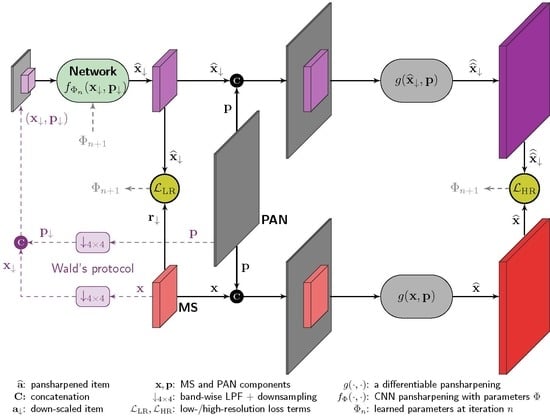
On the basis of the above observations, in this work we propose a training framework that involves also the full-resolution PAN component that, once rescaled, is simply discarded in the previous solutions. Such an integration is achieved by means of a joint low- and high-resolution loss that involves, in the computation of high-resolution loss component, a model-based MRA pansharpening method [20] with good spatial properties. The proposed learning framework is tested on our recently proposed advanced version of PNN [61], hereinafter referred to as A-PNN. In summary, the contributions of this paper are the following:

i.

a new target-adaptive CNN-model for pansharpening with improved capacity at full-resolution;

ii.

a new general learning framework for CNN-based pansharpening that enforces cross-scale consistency;

iii.

an extensive experimental validation for the proposed approach, using two different sensors and a wide variety of comparative solutions, both classical and deep learning.

The rest of the paper is organized as follows. Section 2 introduces the datasets used for training, validation and test, and presents the proposed solution. Section 3 describes the evaluation framework, gathers comparative methods and presents numerical and visual experimental results with related discussion. Section 4 presents further experimental analyses, while Section 5 provides concluding remarks.

2. Materials and Methods

In this section we will describe the datasets used for training, validation and test (Section 2.1). Then, we will present the related work (Section 2.2) to conclude with the proposed method (Section 2.3).

2.1. Datasets

Our proposal starts from the pre-trained networks A-PNN introduced in Reference [61] as advanced versions of PNN, designed for three different imaging systems: GeoEye-1, Ikonos and WorldView-2. In the present work we will focus on GeoEye-1 and WorldView-2 models and datasets.

Table 1. Bandwidths of the multispectral (MS) channels (left-hand side) and Ground Sample Distance [m] at Nadir (rightmost column) for GeoEye-1 (GE1) and WorldView-2 (WV2) images.

	Bandwidths of the MS Channels [nm]								GSD at Nadir [m]
Sensor	Coastal	Red	Blue	Red Edge	Green	Near-IR1	Yellow	Near-IR2	PAN/MS
GE1	-	655–690	450–510	-	510–580	780–920	-	-	0.46/1.84
WV2	400–450	630–690	450–510	705–745	510–580	770–895	585–625	860–1040	0.46/1.84

summarizes the main spectral and spatial characteristics for the target sensors who provide four and eight MS bands, respectively.

The GeoEye-1 A-PNN model was trained and validated on datasets Caserta-GE1-A and -B (near Naples, Italy), respectively, as detailed in

Table 2. Training, validation and test datasets partition. Sizes are in pixels at the scale of the MS component.

	Training/Validation			Test
Sensor	Dataset	Size	Samples	Dataset	Size	Samples
GE1	Caserta-GE1-A/B	33 × 33	14,000/7800	Caserta-GE1-C	320 × 320	15
WV2	Caserta-WV2-A/B	33 × 33	14,000/7800	Washington-WV2	320 × 320	15

. Likewise, the WorldView-2 A-PNN model was trained and validated on a similar partition of a WorldView-2 image of Caserta. For testing our solutions we will use separate image samples (Caserta-GE1-C and Washington-WV2) as detailed in the right-hand side of Table 2. A couple of samples per sensor are shown in Figure 1.

2.2. Background: Target-Adaptive CNN-Based Pansharpening

In this work a new strategy to train CNN models for pansharpening is proposed. In particular we rely on the target-adaptive method A-PNN [61] to prove the effectiveness of the proposed approach. In the following we will therefore briefly recall A-PNN whose network architecture is depicted in Figure 2.

CNNs can be built by combining different processing layers, like convolution, nonlinearities, pooling, deconvolution, batch normalization and so on, according with some direct acyclic graph (DAG). The target-adaptive CNN-based pansharpening algorithm A-PNN is an evolution of the PNN method proposed in Reference [54] which makes use of a three-layer ($L=3$) serial architecture with convolutional layers interleaved by Rectified Linear Unit (ReLU) activations ($max(0,·)$). A-PNN presents in particular three peculiar features with respect to PNN: a different loss for training (L1 instead of L2); a residual learning configuration [63]; a target-adaptive scheme.

The l-th generic convolutional layer, with $N^{\left(l\right)}$-band $H\times W$ input ${\mathbf{u}}^{\left(l\right)}$, yields a $M^{\left(l\right)}\times (H\times W)$ output ${\mathbf{v}}^{\left(l\right)}$ whose m-th band is given by the 2D convolution with bias

$${\mathbf{v}}_m^{\left(l\right)}={\mathbf{w}}_m^{\left(l\right)}\ast {\mathbf{u}}^{\left(l\right)}+b_m^{\left(l\right)},$$

where ${\mathbf{w}}_m^{\left(l\right)}$ is a $(K\times K)\times N^{\left(l\right)}$ convolutional kernel ($K\times K$ is the spatial support), and $b_m^{\left(l\right)}$ is a bias term. For the sake of simplicity, let us indicate with ${\mathsf{\Phi }}^{\left(l\right)}\triangleq ({\mathbf{w}}^{\left(l\right)},{\mathbf{b}}^{\left(l\right)})$, where ${\mathbf{w}}^{\left(l\right)}\triangleq [{\mathbf{w}}_1^{\left(l\right)},\dots ,{\mathbf{w}}_{M^{\left(l\right)}}^{\left(l\right)}]$ and ${\mathbf{b}}^{\left(l\right)}\triangleq [b_1^{\left(l\right)},\dots ,b_{M^{\left(l\right)}}^{\left(l\right)}]$, the set of learnable parameters associated to layer l. Except for the output layer, the convolution variable ${\mathbf{v}}^{\left(l\right)}$ is then passed to the element-wise activation function (ReLU in our case) which provides the l-th set of feature maps ${\mathbf{f}}^{\left(l\right)}$, that is,

$${\mathbf{f}}^{\left(l\right)}\triangleq f_l({\mathbf{u}}^{\left(l\right)},{\mathsf{\Phi }}^{\left(l\right)})=\left\{\begin{array}{cc}max(0,{\mathbf{v}}^{\left(l\right)}),\hfill & l<L\hfill \\ {\mathbf{v}}^{\left(l\right)},\hfill & l=L\hfill \end{array}\right..$$

By concatenating these layer functions (${\mathbf{u}}^{(l+1)}={\mathbf{f}}^{\left(l\right)}$) we get the overall CNN function

$${\tilde{f}}_{\mathsf{\Phi }}\left(\mathbf{u}\right)=f_L(f_{L-1}(\dots f_1(\mathbf{u},{\mathsf{\Phi }}^{\left(1\right)}),\dots ,{\mathsf{\Phi }}^{(L-1)}),{\mathsf{\Phi }}^{\left(L\right)}),$$

(1)

being $\mathsf{\Phi }\triangleq ({\mathsf{\Phi }}^{\left(1\right)},\dots ,{\mathsf{\Phi }}^{\left(L\right)})$ the whole set of parameters to learn. In this chain, each layer l provides a set of feature maps, ${\mathbf{f}}^{\left(l\right)}$, which “activate” on local cues in the early stages (small l), to become more and more representative of global interactions in subsequent ones (large l).

The input $\mathbf{u}={\mathbf{u}}^{\left(1\right)}$ to the network is given by the concatenation of the PAN $\mathbf{p}$ and the upsampled version $\tilde{\mathbf{x}}=\mathrm{up}\left(\mathbf{x}\right)$ of the MS component $\mathbf{x}$:

$$\mathbf{u}\triangleq (\tilde{\mathbf{x}},\mathbf{p}).$$

On the other hand, the actual output $\widehat{\mathbf{x}}$ is the sum of the output of the last convolutional layer, ${\mathbf{f}}^{\left(L\right)}$ and $\tilde{\mathbf{x}}$, as shown in Figure 2, yielding

$$\widehat{\mathbf{x}}=\tilde{\mathbf{x}}+{\mathbf{f}}^{\left(L\right)}=\tilde{\mathbf{x}}+{\tilde{f}}_{\mathsf{\Phi }}\left(\mathbf{u}\right).$$

(2)

By doing so, the network is asked to predict only the missing detail $\widehat{\mathbf{x}}-\tilde{\mathbf{x}}$, resulting in a much faster training process (known in the literature as residual learning). For the sake of simplicity, we will refer to the function $f_{\mathsf{\Phi }}$ that incorporates the polynomial upsampling of the MS component, $\tilde{\mathbf{x}}$ and the skip connection for residual learning, which directly depends on the two input components $\mathbf{x}$ and $\mathbf{p}$ as shown in Figure 2. In formal terms,

$$\widehat{\mathbf{x}}=f_{\mathsf{\Phi }}(\mathbf{x},\mathbf{p})\triangleq \tilde{\mathbf{x}}+{\tilde{f}}_{\mathsf{\Phi }}\left(\left(\mathrm{up}\right(\mathbf{x}),\mathbf{p})\right).$$

(3)

The main hyper-parameters of A-PNN for WorldView-2 are gathered in

Table 3. Hyper-parameters of the A-PNN model [61] for WorldView-2 images.

Layer	Spatial Support	Input Bands	Output Features	Activation
	($\mathit{K}\mathbf{\times }\mathit{K}$)	(${\mathit{N}}^{\mathbf{\left(}\mathit{l}\mathbf{\right)}}$)	(${\mathit{M}}^{\mathbf{\left(}\mathit{l}\mathbf{\right)}}$)
$l=1$	$9\times 9$	9	48	ReLU
$l=2$	$5\times 5$	48	32	ReLU
$l=3$	$5\times 5$	32	8	none

(see Reference [61] for other sensors).

In order to train the network parameters $\mathsf{\Phi }$, a sufficiently large number of input-output (labeled) examples is required. Lacking ideally pansharpened images to be used as references, A-PNN and other CNN-based methods resort to a sample generation strategy where the scale of the training dataset is reduced by a factor equal to the PAN-MS resolution ratio, allowing the original MS data to play the role of reference. Once trained, the network is ready to be used to pansharpen any image at its own resolution.

As a peculiar trait, A-PNN allows one to refine parameters on the target image according with the top-level workflow depicted in Figure 3. At test time the process starts with a net pre-trained on a generic dataset (see Table 2). The initial parameters, ${\mathsf{\Phi }}_0$, are then refined with 50 iterations on a reduced-resolution version of the target image, which takes just a few seconds even for large targets. Then, the pansharpening of the input at its native resolution is eventually performed using the refined parameters, say ${\mathsf{\Phi }}_{\infty }$, achieving a significant performance gain. Both pre-training and fine-tuning are carried out using a $L_1$-norm which corresponds to the mean absolute error between the reference image and the pansharpening result. For additional details about training the Reader is referred to References [54,61].

2.3. Proposed Method

Among the most critical aspects of deep learning methods for super-resolution or pansharpening there is the capability to generalize from the training resolution to the test resolution. As explained above, the training set is generally obtained by means of a resolution shift (called Wald’s protocol [62] in the case of pansharpening). This same reasoning is also encoded in the fine-tuning stage of A-PNN as depicted in Figure 3. For general purpose super-resolution tasks the scale-generalization problem is less critical thanks to the abundance of training data, typically spanning a wide range of spatial resolutions. Instead, in case of remotely sensed images this becomes a serious issue as all sample images are taken at a fixed distance from the ground, hence at a nearly constant ground sample distance. Put in simpler words, tiny objects whose size amounts to a few pixels at the scale of the PAN (think of cars, horizontal traffic signs, etc.) would loose their geometry or disappear at the end of a resolution downgrading process used to generate training samples. As a result, no representative occurrences of these elements will be observed in the training dataset, with a consequent misalignment between training and test datasets. To this regard, it should not surprise that the large gain of CNN-based methods over traditional approaches in the reduced resolution evaluation framework [50,54,56,59,61] comes with a less clear-cut gain in the full-resolution context [59,61].

A few attempts to deal with this issue have been carried out for both super-resolution [64] and pansharpening [65]. In both cases the underlying idea was to involve an additional loss term that accounts for the target-resolution behaviour of the network. By following a similar rationale we propose here a training scheme which is summarized in Figure 4. In particular, we decided to apply this training scheme directly in the fine-tuning phase of the pre-trained A-PNN network with parameters ${\mathsf{\Phi }}_0$. (We refer to the pretrained network available online at: https://github.com/sergiovitale/pansharpening-cnn-python-version). This choice is motivated by the fact that the performance loss due to the misalignment between training and test sets can be very large, so that the fine-tuning by-itself impacts considerably on the final performance.

Eventually, in the fine-tuning stage, in addition to the term ${\mathcal{L}}_{\mathrm{LR}}$ defined in the reduced-resolution domain, we also consider a full-resolution term ${\mathcal{L}}_{\mathrm{HR}}$ obtained by suitably processing the target image $(\mathbf{x},\mathbf{p})$ according to the scheme of Figure 4:

$$\mathcal{L}=\alpha {\mathcal{L}}_{\mathrm{LR}}+\beta {\mathcal{L}}_{\mathrm{HR}}.$$

${\mathcal{L}}_{\mathrm{LR}}$ is the same loss term computed in the original A-PNN fine-tuning stage (Figure 3) in the low resolution (LR) domain,

$${\mathcal{L}}_{\mathrm{LR}}={∥{\widehat{\mathbf{x}}}_{\downarrow }-{\mathbf{r}}_{\downarrow }∥}_1={∥f_{{\mathsf{\Phi }}_n}({\mathbf{x}}_{\downarrow },{\mathbf{p}}_{\downarrow })-\mathbf{x}∥}_1,$$

which is replaced by its average over minibatches in normal (pre-)training. Instead, the high resolution (HR) loss term is derived in the full-resolution space as

$${\mathcal{L}}_{\mathrm{HR}}={∥{\widehat{\widehat{\mathbf{x}}}}_{\downarrow }-\widehat{\mathbf{x}}∥}_1={∥g({\widehat{\mathbf{x}}}_{\downarrow },\mathbf{p})-g(\mathbf{x},\mathbf{p})∥}_1={∥g(f_{{\mathsf{\Phi }}_n}({\mathbf{x}}_{\downarrow },{\mathbf{p}}_{\downarrow }),\mathbf{p})-g(\mathbf{x},\mathbf{p})∥}_1,$$

where the pansharpening at target-resolution is performed with a fixed differentiable function $g(·,·)$. In particular, we decided to use one of the conventional solutions that show very good performance on spatial enhancement which is the MTF-GLP-HPM model-based approach proposed in Reference [20] and made available in the toolbox associated with the pansharpening survey by Vivone et al. [3]. In fact, this method strongly relies on the detail information conveyed by the PAN component while limiting spectral distortion phenomena.

By doing so, we enforce cross-scale consistency thanks to the joint training on low and high resolution data. To clarify this point, think of a simplified case where ${\mathcal{L}}_{\mathrm{LR}}=ϵ$ with constant $ϵ>0$. The simultaneous minimization of ${\mathcal{L}}_{\mathrm{HR}}$ allows to favor, among all possible solutions ${\widehat{\mathbf{x}}}_{\downarrow }$, the one that better fuses with the full-resolution PAN $\mathbf{p}$ from the perspective of a reference pansharpening method (MTF-GLP-HM). Put in different words, we may say that the combined loss seeks to indirectly balance the A-PNN behaviour, at reduced scale, with that of a model-based approach with nice spatial characteristics, at full scale. The balance of the two loss terms (norms are intended already normalized by pixel) is obtained by setting equal weights, $\alpha =\beta =1$, having experimentally found on several test images that the two loss contributions are already roughly balanced at the begin of the fine-tuning process. The fine-tuning runs for 50 epochs on the target image starting from the initial parameter configuration ${\mathsf{\Phi }}_0$ inherited from the A-PNN model. In particular an Adam optimizer [66] with a learning rate equal to 0.0003 and momentums ${\beta }_1=0.9$ and ${\beta }_2=0.99$ is employed. Each test image will therefore be associated to a different, adapted, parameters configuration ${\mathsf{\Phi }}_{\infty }$.

Finally, notice also that the proposed loss involves the full-resolution PAN component $\mathbf{p}$, a data term which is simply discarded by early CNN approaches to pansharpening including our baseline A-PNN, a relevant fact by itself, since the precious information conveyed by this component is not taken into account otherwise.

3. Experimental Validation

In this section, first we will briefly recall the accuracy evaluation metrics employed (Section 3.1) and the comparative methods (Section 3.2), then we will provide and discuss numerical and visual results (Section 3.3).

3.1. Accuracy Metrics

The numerical assessment of pansharpening methods is commonly carried out on two resolution levels [3]: the target, or full, resolution level corresponding to the actual resolution of the dataset at hand, and the reduced resolution level obtained by scaling the data with a factor R (PAN-MS resolution ratio) resorting to Wald’s protocol [62]. In the full-resolution framework only qualitative measurements (no-reference indexes) are usually possible because of the lack of ground-truth images (ideally pansharpened references). As a consequence, in order to compute objective error measurements (reference-based indexes) it is customary to use Wald’protocol and work in the reduced resolution domain, where the original MS component plays as ground-truth. On the other hand, in addition to the numerical assessment it is always useful to visually inspect sample results at both scales to detect local artefacts that may not be recognized by globally averaged measurements.

In particular, we will make use of the following reference-based metrics in the reduced resolution space:

• Universal Image Quality Index (Q-index) which takes into account three different components: correlation coefficient, mean luminance distance and contrast [67].
• Erreur Relative Globale Adimensionnelle de Synthése (ERGAS) which measures the overall radiometric distortion between two images [68].
• Spectral Angle Mapper (SAM) which measures the spectral divergence between images by averaging the pixel-wise angle between spectral signatures [69].
• Q4/Q8, a 4/8 bands extension of the universal image quality index [70].

On the other hand, the no-reference indexes employed in full-resolution framework will be the following [3,71]:

• Quality No-Reference (QNR) index, is a combination of two indexes that take into account spatial and spectral distortions, DS and D${}_{\mathbf{\lambda }}$, respectively:

  –

  Spectral Distortion (D${}_{\mathbf{\lambda }}$), measures the distance of the bands correlation between $\widehat{\mathbf{x}}$ and $\tilde{\mathbf{x}}$.

  –

  Spatial Distortion (D${}_{\mathit{S}}$), measures the spatial consistency between the $\widehat{\mathbf{x}}$ and $\mathbf{p}$.

For further details about the definition of the above indexes the Reader is referred to the corresponding references.

3.2. Compared Methods

Traditional approaches to pansharpening include component substitution, multiresolution analysis, statistical or variational approaches and other hybrid solutions. A critical survey on these methods can be found in [3]. On the other hand, many deep learning solutions have been proposed in the last years. In this work we compare the proposed method with both traditional and deep learning methods. In particular we have selected the methods listed in

Table 4. Comparative methods.

Model-Based Methods
ATWT-M3 [15]	A Troús Wavelet Transform-based method
AWLP [17]	Additive Wavelet Luminance Proportional method
BDSD [14]	Band-Dependent Spatial-Detail with local parameter estimation method
C-BDSD [26]	A non-local extension of BDSD
GSA [12]	A Gram-Schmidt-based Algorithm
Indusion [18]	Decimated Wavelet Transform using an additive injection model
PRACS [13]	Partial Replacement Adaptive Component Substitution
MTF-GLP-HPM [20]	MTF-tailored Generalized Laplacian Pyramid with HP Modulation injection
Deep Learning Methods
DRPNN [55]	Deep Residual Pansharpening Neural Network
PanNet [50]	Pansharpening Network
A-PNN [61]	Target-Adaptive PNN

that are representative examples of these groups.

3.3. Results and Discussion

According with Table 2 we compare our solution on two test datasets, Caserta-GE1-C and Washington-WV2, each composed of fifteen image samples whose MS (PAN) component is 320 × 320 (1280 × 1280) pixels wide. The corresponding samples in the reduced resolution evaluation framework will therefore have size 80 × 80 (320 × 320) pixels.

Let us start with the numerical results obtained at both full and reduced resolutions which are gathered in

Table 5. Numerical results on Caserta-GE1-C dataset at full (left-hand side) and reduced (right-hand side) resolutions. Best figures are highlighted with bold numbers, while second best ones are underlined.

	Full Resolution			Reduced Resolution
	D${}_{\mathit{\lambda }}$	D${}_{\mathit{S}}$	QNR	Q4	Q	SAM	ERGAS
(Ideal Value)	(0)	(0)	(1)	(1)	(1)	(0)	(0)
ATWT-M3	0.0831	0.0837	0.8408	0.7846	0.5787	3.1212	2.8566
AWLP	0.1241	0.1716	0.7259	0.8502	0.6921	3.6143	2.6248
BDSD	0.0583	0.1105	0.8383	0.8713	0.7171	3.0415	2.1226
C-BDSD	0.0991	0.1562	0.7611	0.8637	0.7142	3.2020	2.3013
GSA	0.1218	0.2026	0.7008	0.8039	0.6683	3.9410	2.7130
Indusion	0.1344	0.1481	0.7390	0.7667	0.5550	3.3720	3.4209
PRACS	0.0506	0.0995	0.8553	0.8419	0.6677	2.8774	2.3334
MTF-GLP-HPM	0.1120	0.1051	0.7946	0.9069	0.8353	3.3242	2.1747
DRPNN	0.0347	0.0577	0.9097	0.8817	0.7205	3.0791	3.0165
PanNet	0.0504	0.1088	0.8472	0.7758	0.5846	3.4378	2.8738
A-PNN	0.0335	0.0597	0.9089	0.9460	0.8102	1.7842	1.3564
Proposed	0.0336	0.0517	0.9199	0.9305	0.7786	2.2612	1.6612

for the GeoEye-1 dataset and in

Table 6. Numerical results on Washington-WV2 dataset at full (left-hand side) and reduced (right-hand side) resolutions. Best figures are highlighted with bold numbers, while second best ones are underlined.

	Full Resolution			Reduced Resolution
	D${}_{\mathit{\lambda }}$	D${}_{\mathit{S}}$	QNR	Q8	Q	SAM	ERGAS
(Ideal Value)	(0)	(0)	(1)	(1)	(1)	(0)	(0)
ATWT-M3	0.0676	0.1286	0.8126	0.7087	0.5953	7.7816	5.7164
AWLP	0.0738	0.1209	0.8144	0.8293	0.7425	6.8673	4.3049
BDSD	0.0685	0.1096	0.8298	0.8455	0.7524	7.4456	4.2333
C-BDSD	0.0429	0.0421	0.9169	0.8408	0.7505	7.7323	4.5232
GSA	0.0421	0.1350	0.8287	0.7598	0.6957	8.4762	5.0132
Indusion	0.0696	0.1077	0.8302	0.7773	0.6565	7.2221	5.2228
PRACS	0.0117	0.0927	0.8967	0.7462	0.6357	7.0986	5.0136
MTF-GLP-HPM	0.0838	0.1387	0.7892	0.8412	0.7590	6.7925	4.0543
DRPNN	0.0471	0.0853	0.8721	0.8664	0.5277	6.6549	4.2072
PanNet	0.0341	0.1052	0.8645	0.8140	0.7169	6.8125	4.6004
A-PNN	0.0430	0.0495	0.9098	0.8459	0.9236	4.4567	2.6353
Proposed	0.0313	0.0506	0.9196	0.9015	0.8132	4.9994	3.0485

for the WorldView-2 images. Each number is the average value over the related fifteen samples. Among the model-based approaches, PRACS and C-BDSD provide the best performance in the full resolution framework on GeoEye-1 and WorldView-2 datasets, respectively. However, the latter provides also fairly good results in the reduced resolution context. Such a good trade-off between reference-based and no-reference accuracies is also a feature of BDSD on GeoEye-1 images. On the other hand, according to the objective error measurements at reduced resolution, MTF-GLP-HPM provides a superior performance which is consistent over the different indicators and datasets.

Moving to deep learning methods, our baseline, A-PNN and the proposed method get the best overall performance considering both no-reference and reference-based assessments, and for both datasets. In particular, the proposal provides the highest accuracy in the full resolution framework (the QNR is the main indicator to look at, which summarizes spatial and spectral fidelity) while A-PNN performs generally better according to reference-based indicators. This relative positioning of the proposal with respect to A-PNN is coherent with the proposed loss which balances reduced-resolution and full-resolution costs in order to provide cross-scale consistency. Between the two remaining deep learning solutions, DRPNN outperforms PanNet which seem to suffer on our datasets, whereas it provides better scores on other datasets [50]. This performance variability of deep learning methods with respect to the dataset was investigated in Reference [61] and motivates further the use of target-adaptive schemes such as A-PNN and the proposal. Overall, with the exception of A-PNN and proposal which outperform consistently all methods, the gap between deep learning methods and the others is not always clear-cut.

For a more comprehensive evaluation of the methods, a careful visual inspection of results is necessary besides numerical assessment, in order to study local patterns and visual artifacts that may not emerge from global averages. To this aim, Figure 5 and Figure 6 show some pansharpening results on crops from Caserta-GE1-C and Washington-WV2 images, respectively, at reduced resolution. In particular, for the sake of brevity, we limit the visual analysis to the methods that are more competitive and/or are related to our proposal. These are deep learning methods, MTF-GLP-HPM, which is also involved in the definition of the proposed loss and C-BDSD which is one of the best model-based approaches. For each of the stacked examples the target ground-truth is shown on the leftmost column, followed by the different pansharpening results, with the associated error map shown below. As it can be seen, PanNet introduces a rather visible spatial distortion on GeoEye-1 samples (Figure 5), which is also present to a minor extent on WorldView-2 tiles (Figure 6). This agrees with the reduced resolution numerical figures reported in Table 5 and Table 6. Although of less intensity, spatial distortions are also clearly visible for C-BDSD, DRPNN and MTF-GLP-HPM, which outperform PanNet at the reduced scale. On the other hand, coherently with the best performance shown in the reduced resolution frame, A-PNN provides the highest fidelity with a nearly zero error map. Finally, the proposed solution gets results that look close to A-PNN in some cases. Some variations in the error maps are also visible for our method which can be justified by the introduction of the additional loss term that operates in the full resolution space for cross-scale consistency.

With the help of Figure 7 and Figure 8, we can now analyze some results obtained at the target full resolution. Unfortunately, at this scale there are no reference images and all considerations are necessarily subjective. Ideally, a good pansharpening should be able to provide the spatial detail level of the PAN while keeping the spectral response of the ground objects according to the MS image. Therefore, in Figure 7 and Figure 8 we show the PAN and MS components as reference for each sample in the first two columns. Then, several compared pansharpening results are shown moving rightward. With the premises made above, we formulate the following observations.

Overall, the compared methods seem to provide quite similar performances on the GeoEye-1 dataset. Differences are therefore quite subtle and difficult to be noticed. In particular, C-BDSD, MTF-GLP-HPM and PanNet present a tendency to over-emphasize spatial details. This is particularly visible for PanNet which introduces also micro-textural patterns. Such a feature is somehow reflected in the spatial distortion indicator D${}_{\mathit{S}}$ (Table 5) which almost doubles for these three methods in comparison to the other selected methods. On the contrary, DRPNN results look too smooth, while A-PNN and the proposed method seem to give sharpness levels which are closer to that of the PAN image, with the proposed being sharper than A-PNN, as it can be seen in the last example.

On WorldView-2 images (Figure 8) some of the above considerations still apply but are much easier to be seen. In particular, the smoothness of DRPNN, as well as the over-emphasis on spatial details of C-BDSD are clearly visible. Here, PanNet and MTF-GLP-HPM provide much better spatial descriptions, sharper for the former, smoother for the latter. Finally, A-PNN and the proposed method look in between PanNet and MTF-GLP-HPM in terms of spatial details. However, A-PNN presents a visible spectral distortion particularly evident on vegetated areas.

On the basis of the above discussion on numerical and visual results at both full and reduced resolution, we can conclude that A-PNN and its variant proposed in this work show the most robust behaviour across scales and sensors. Besides, we have to keep in mind that the evaluation of pansharpening methods is itself still an open problem, since objective error measurements are only possible at the reduced scale which is not the target one. For this reason, our goal was to improve the full resolution performance by means of a suitably defined cross-scale training process, although we had to suffer a slight loss in the reduced resolution framework. In contrast, we observed an improvement in both numerical and visual terms, reducing spectral distortions, in the case of WorldView-2, and spatial blur, for GeoEye-1. Moreover, the proposed solution can be easily generalized to different mappings $g(·)$ (MTF-GLP-HPM, in this work) which do not necessarily need to be a pansharpening function. It could be, for example, any kind of differentiable detector or whatever feature extractor defined on multispectral images. In this last case one can adapt the pansharpening network to the user application.

4. Further Analyses

In this section we present complementary results for a more comprehensive evaluation of the proposed method. In particular, we provide three additional analyses: a comparison restricted to the DL methods where the fine-tuning is used for all, an ablation study for the proposal and an assessment of the computational burden.

In the previous section the proposed solution has been compared to both traditional and DL models. DL models have been taken already pre-trained as provided by the authors. Therefore, criticisms could be made of this approach to the comparison of DL models. In fact, in the computer vision community it is customary to fix both training and test datasets to ensure that all compared model access to the same information in the learning phase. Unfortunately, this way to proceed cannot always be extended to the remote sensing domain because of the restrive policies frequently occurring. This is also the case here. Of course, we could train from scratch on our datasets all compared models but this would open many issues such as “is our dataset properly sized to train others’ models?” Deeper networks, in fact, require larger datasets to avoid overfitting. Or, “is our training schedule suited to let others’ models converge properly?” Letting a DL model to “converge” toward a reasonably small loss is never an easy task and requires usually an extensive trial and error process. If this job is not carried out by the same authors that have conceived the model, who are confident with it, there is a high risk to penalize the model.

Aware of the above mentioned issues, we decided to make a further comparison by extending the fine-tuning stage to all DL solutions.

Table 7. Numerical comparison of the fine-tuned deep learning (DL) models at full (left-hand side) and reduced (right-hand side) resolutions. Best figures are highlighted with bold numbers, while second best ones are underlined.

		Full Resolution			Reduced Resolution
Dataset	Model	D${}_{\mathit{\lambda }}$	D${}_{\mathit{S}}$	QNR	Q4	Q	SAM	ERGAS
		(0)	(0)	(1)	(1)	(1)	(0)	(0)
GE1	DRPNN	0.0623	0.0745	0.8680	0.9097	0.7480	2.3163	1.9042
	PanNet	0.0799	0.1099	0.8194	0.9057	0.7317	2.4496	1.7031
	A-PNN	0.0335	0.0597	0.9089	0.9460	0.8102	1.7842	1.3564
	Proposed	0.0336	0.0517	0.9199	0.9305	0.7786	2.2612	1.6612
WV2	DRPNN	0.0397	0.1082	0.8566	0.9103	0.8230	4.7301	2.8100
	PanNet	0.0326	0.0772	0.8927	0.8933	0.7925	5.4700	3.1499
	A-PNN	0.0430	0.0495	0.9098	0.8459	0.9236	4.4567	2.6353
	Proposed	0.0313	0.0506	0.9196	0.9015	0.8132	4.9994	3.0485

gathers the numerical results obtained on the test images of GeoEye-1 and WorldView-2, at both resolutions. A-PNN and the proposed model have been already comparatively discussed in the previous section with the overall conclusion that the latter performs better in the full-resolution domain on both sensors. Moving to DRPNN and PanNet, observe first that all reduced resolution indexes register a large gain with respect to the non fine-tuned versions (compare with Table 5 and Table 6), particularly DRPNN on WorldView-2. This is perfectly in line with our expectations since the fine-tuning occurs on the reduced resolution test image. However, this comes at the cost of a large performance loss at full-resolution (except for PanNet on WorldView-2). Here, to have an idea, the QNR drops from about 0.91 to 0.87 for DRPNN on GeoEye-1. In essence, this reflects an overfitting of the models on the reduced-resolution samples, which is much heavier for deeper networks like DRPNN and PanNet. This phenomenon, which was also observed to a much smaller extent for A-PNN in the original work [61], allows us to further appreciate the mitigating contribute of the full-resolution loss component ${\mathcal{L}}_{\mathrm{HR}}$ that acts as regularization term, keeping high accuracy levels at the target scale.

Besides, it is also worth to assess the marginal contribute of the two loss components involved in the proposed learning scheme. In

Table 8. Ablation Study on Caserta-GE1-C and Washington-WV2. The proposed model is fine-tuned using ${\mathcal{L}}_{\mathrm{LR}}$ (A-PNN), ${\mathcal{L}}_{\mathrm{HR}}$ or both (proposal).

		Full Resolution			Reduced Resolution
Dataset	Loss	D${}_{\mathit{\lambda }}$	D${}_{\mathit{S}}$	QNR	Q4/Q8	Q	SAM	ERGAS
		(0)	(0)	(1)	(1)	(1)	(0)	(0)
GE1	${\mathcal{L}}_{\mathrm{LR}}$ (A-PNN)	0.0335	0.0597	0.9089	0.9460	0.8102	1.7842	1.3564
	${\mathcal{L}}_{\mathrm{HR}}$	0.0337	0.0518	0.9163	0.9305	0.7786	2.2632	1.6641
	${\mathcal{L}}_{\mathrm{LR}}$ + ${\mathcal{L}}_{\mathrm{HR}}$ (Proposed)	0.0336	0.0517	0.9199	0.9305	0.7786	2.2612	1.6612
WV2	${\mathcal{L}}_{\mathrm{LR}}$ (A-PNN)	0.0430	0.0495	0.9098	0.8459	0.9236	4.4567	2.6353
	${\mathcal{L}}_{\mathrm{HR}}$	0.0348	0.0504	0.9165	0.9006	0.8098	5.1197	3.1272
	${\mathcal{L}}_{\mathrm{LR}}$ + ${\mathcal{L}}_{\mathrm{HR}}$ (Proposed)	0.0313	0.0506	0.9196	0.9015	0.8132	4.9994	3.0485

the proposed model is compared with its ablated versions obtained training on a single loss term. As it can be seen, the use of the ${\mathcal{L}}_{\mathrm{HR}}$ component alone is sufficient to gain accuracy at full resolution, although it comes with a larger performance loss in the reduce-resolution frame. The joint optimization, instead, allows also to preserve to some extent the performance at reduced resolution.

Last but not least, a look to the computational burden allows us to have a complete picture of our proposal. To this aim we have run dedicated tests to quantify experimentally the computational time needed by each compared method on fixed hardware and image size (1280 × 1280 at PAN scale). In particular, we have considered both CPU and GPU equipped computers.

Table 9. Running time (seconds) for DL methods on CPU and GPU. Time overload due to the fine-tuning phase is given within brackets.

Device	DRPNN	PanNet	A-PNN	Proposed
CPU: AMD 1950X (4 active cores)	4 (+400)	2.7 (+100)	9 (+70)	9 (+1750)
GPU: GeForce GTX 1080 Ti (12 GB)	2 (+20)	2.3 (+4.5)	0.25 (+0.75)	0.25 (+14)

summarizes the running time for DL methods, telling apart (within brackets) the additional contribute due to the fine-tuning. The other non-DL methods were tested on CPU only showing an execution time ranging from half a second (Indusion, GSA, BDSD) to about six seconds (ATWT-M3). As expected, due to their inherent complexity, deep learning methods are much slower than non-DL ones on CPU, with the fine-tuning phase responsible for the dominant cost. On the other hand, we can resort to parallel implementations for these methods and hence rely on the use of GPUs to save time. In particular, observe that two main aspects impact on complexity: the network size and the batch size for parameters training. Here, DRPNN and PanNet are much deeper than A-PNN and proposal. On the other hand, different from the others, the proposed model is trained using the full-resolution version of the target image, hence requiring a 16 times larger batch. This latter observation explains why the proposal, although sharing the same (relatively small) architecture of A-PNN, is computationally much more expensive. To conclude, we have also to underline that the focus of this work was on accuracy rather than on complexity. Therefore, there is a room left for improvement from the computational perspective, for example using cropping strategies to reduce the volume of the image to be used in fine-tuning, or resorting to mini-batch decompositions, since the current implementation relies on a single-batch optimization schedule.

5. Conclusions

In this work we have proposed an enhanced version of the CNN-based method A-PNN. This contribution comes with the introduction of a new learning scheme that can be straightforwardly extended to any CNN model for pansharpening. The new learning scheme involves loss terms computed at reduced and full resolutions, respectively, enforcing cross-scale consistency. Our experiments show a clear performance improvement over the single-scale training scheme in the full-resolution evaluation framework according to both numerical and visual assessments. This achievement is paid with an increased computational cost and a negligible accuracy loss in the reduced-scale domain, which is in principle not an issue in real-world practical applications as full-resolution images are concerned. Moreover, numerical and visual results confirm the superior accuracy levels achievable by DL-based solutions in comparison to traditional model-based approaches, with the proposed one being the best in the full-resolution evaluation framework, and its baseline A-PNN being the best in the reduced-resolution domain.

There is a room left for the improvement of the proposed learning scheme that is worth to explore in future work. First, the increased computational cost can be limited by means of a suitable cropping strategy aimed to reduce the volume of data to be processed. Second, different auxiliary fusion functions $g(·,·)$ can be tested, which do not necessarily have to be pansharpening models. For example any application-oriented feature extractor which is differentiable (to allow gradient backpropagation) may also be used, allowing for an application-driven learning. Finally, needless to say, many different core CNN models can be tested in place of A-PNN.

References

1. Gargiulo, M.; Mazza, A.; Gaetano, R.; Ruello, G.; Scarpa, G. A CNN-Based Fusion Method for Super-Resolution of Sentinel-2 Data. In Proceedings of the IGARSS 2018—2018 IEEE International Geoscience and Remote Sensing Symposium, Valencia, Spain, 22–27 July 2018; pp. 4713–4716. [Google Scholar] [CrossRef]
2. Errico, A.; Angelino, C.V.; Cicala, L.; Podobinski, D.P.; Persechino, G.; Ferrara, C.; Lega, M.; Vallario, A.; Parente, C.; Masi, G.; et al. SAR/multispectral image fusion for the detection of environmental hazards with a GIS. In Proceedings of the SPIE—The International Society for Optical Engineering, Amsterdam, The Netherlands, 23 October 2014; Volume 9245. [Google Scholar]
3. Vivone, G.; Alparone, L.; Chanussot, J.; Mura, M.D.; Garzelli, A.; Licciardi, G.A.; Restaino, R.; Wald, L. A Critical Comparison Among Pansharpening Algorithms. IEEE Trans. Geosci. Remote Sens. 2015, 53, 2565–2586. [Google Scholar] [CrossRef]
4. Gaetano, R.; Amitrano, D.; Masi, G.; Poggi, G.; Ruello, G.; Verdoliva, L.; Scarpa, G. Exploration of multitemporal COSMO-skymed data via interactive tree-structured MRF segmentation. IEEE J. Sel. Top. Appl. Earth Obs. Remote Sens. 2014, 7, 2763–2775. [Google Scholar] [CrossRef]
5. Aiazzi, B.; Alparone, L.; Baronti, S.; Garzelli, A.; Selva, M. MTF-tailored multiscale fusion of high-resolution MS and Pan imagery. Photogramm. Eng. Remote Sens. 2006, 72, 591–596. [Google Scholar] [CrossRef]
6. Shettigara, V. A generalized component substitution technique for spatial enhancement of multispectral images using a higher resolution data set. Photogramm. Eng. Remote Sens. 1992, 58, 561–567. [Google Scholar]
7. Tu, T.M.; Su, S.C.; Shyu, H.C.; Huang, P.S. A new look at IHS-like image fusion methods. Inf. Fusion 2001, 2, 177–186. [Google Scholar] [CrossRef]
8. Tu, T.M.; Huang, P.S.; Hung, C.L.; Chang, C.P. A fast intensity hue-saturation fusion technique with spectral adjustment for IKONOS imagery. IEEE Geosci. Remote Sens. Lett. 2004, 1, 309–312. [Google Scholar] [CrossRef]
9. Chavez, P.; Kwarteng, A. Extracting spectral contrast in Landsat thematic mapper image data using selective principal component analysis. Photogramm. Eng. Remote Sens. 1989, 55, 339–348. [Google Scholar]
10. Gillespie, A.R.; Kahle, A.B.; Walker, R.E. Color enhancement of highly correlated images. II. Channel ratio and “chromaticity” transformation techniques. Remote Sens. Environ. 1987, 22, 343–365. [Google Scholar] [CrossRef]
11. Laben, C.; Brower, B. Process for Enhancing the Spatial Resolution of Multispectral Imagery Using Pan-Sharpening. U.S. Patent 6011875, 4 January 2000. [Google Scholar]
12. Aiazzi, B.; Baronti, S.; Selva, M. Improving component substitution pansharpening through multivariate regression of MS+Pan data. IEEE Trans. Geosci. Remote Sens. 2007, 45, 3230–3239. [Google Scholar] [CrossRef]
13. Choi, J.; Yu, K.; Kim, Y. A New Adaptive Component-Substitution-Based Satellite Image Fusion by Using Partial Replacement. IEEE Trans. Geosci. Remote Sens. 2011, 49, 295–309. [Google Scholar] [CrossRef]
14. Garzelli, A.; Nencini, F.; Capobianco, L. Optimal MMSE pan sharpening of very high resolution multispectral images. IEEE Trans. Geosci. Remote Sens. 2008, 46, 228–236. [Google Scholar] [CrossRef]
15. Ranchin, T.; Wald, L. Fusion of high spatial and spectral resolution images: The ARSIS concept and its implementation. Photogramm. Eng. Remote Sens. 2000, 66, 49–61. [Google Scholar]
16. Nunez, J.; Otazu, X.; Fors, O.; Prades, A.; Pala, V.; Arbiol, R. Multiresolution-based image fusion with additive wavelet decomposition. IEEE Trans. Geosci. Remote Sens. 1999, 37, 1204–1211. [Google Scholar] [CrossRef] [Green Version]
17. Otazu, X.; Gonzalez-Audicana, M.; Fors, O.; Nunez, J. Introduction of sensor spectral response into image fusion methods. Application to wavelet-based methods. IEEE Trans. Geosci. Remote Sens. 2005, 43, 2376–2385. [Google Scholar] [CrossRef] [Green Version]
18. Khan, M.; Chanussot, J.; Condat, L.; Montanvert, A. Indusion: Fusion of Multispectral and Panchromatic Images Using the Induction Scaling Technique. IEEE Geosci. Remote Sens. Lett. 2008, 5, 98–102. [Google Scholar] [CrossRef] [Green Version]
19. Aiazzi, B.; Alparone, L.; Baronti, S.; Garzelli, A. Context-driven fusion of high spatial and spectral resolution images based on oversampled multiresolution analysis. IEEE Trans. Geosci. Remote Sens. 2002, 40, 2300–2312. [Google Scholar] [CrossRef]
20. Aiazzi, B.; Alparone, L.; Baronti, S.; Garzelli, A.; Selva, M. An MTF-based spectral distortion minimizing model for pan-sharpening of very high resolution multispectral images of urban areas. In Proceedings of the GRSS/ISPRS Joint Workshop on Remote Sensing and Data Fusion over Urban Areas, Berlin, Germany, 22–23 May 2003; pp. 90–94. [Google Scholar]
21. Lee, J.; Lee, C. Fast and Efficient Panchromatic Sharpening. IEEE Trans. Geosci. Remote Sens. 2010, 48, 155–163. [Google Scholar] [CrossRef]
22. Restaino, R.; Mura, M.D.; Vivone, G.; Chanussot, J. Context-Adaptive Pansharpening Based on Image Segmentation. IEEE Trans. Geosci. Remote Sens. 2017, 55, 753–766. [Google Scholar] [CrossRef] [Green Version]
23. Shah, V.P.; Younan, N.H.; King, R.L. An Efficient Pan-Sharpening Method via a Combined Adaptive PCA Approach and Contourlets. IEEE Trans. Geosci. Remote Sens. 2008, 46, 1323–1335. [Google Scholar] [CrossRef]
24. Fasbender, D.; Radoux, J.; Bogaert, P. Bayesian Data Fusion for Adaptable Image Pansharpening. IEEE Trans. Geosci. Remote Sens. 2008, 46, 1847–1857. [Google Scholar] [CrossRef]
25. Zhang, L.; Shen, H.; Gong, W.; Zhang, H. Adjustable Model-Based Fusion Method for Multispectral and Panchromatic Images. IEEE Trans. Syst. Man Cybern. B Cybern. 2012, 42, 1693–1704. [Google Scholar] [CrossRef] [PubMed]
26. Garzelli, A. Pansharpening of Multispectral Images Based on Nonlocal Parameter Optimization. IEEE Trans. Geosci. Remote Sens. 2015, 53, 2096–2107. [Google Scholar] [CrossRef]
27. Meng, X.; Shen, H.; Li, H.; Yuan, Q.; Zhang, H.; Zhang, L. Improving the Spatial Resolution of Hyperspectral Image Using Panchromatic and Multispectral Images: An Integrated Method; WHISPERS: Los Angeles, CA, USA, 2015. [Google Scholar]
28. Shen, H.; Meng, X.; Zhang, L. An Integrated Framework for the Spatio-Temporal-Spectral Fusion of Remote Sensing Images. IEEE Trans. Geosci. Remote Sens. 2016, 54, 7135–7148. [Google Scholar] [CrossRef]
29. Zhong, S.; Zhang, Y.; Chen, Y.; Wu, D. Combining Component Substitution and Multiresolution Analysis: A Novel Generalized BDSD Pansharpening Algorithm. IEEE J. Sel. Top. Appl. Earth Obs. Remote Sens. 2017, 10, 2867–2875. [Google Scholar] [CrossRef]
30. Palsson, F.; Sveinsson, J.; Ulfarsson, M. A New Pansharpening Algorithm Based on Total Variation. IEEE Geosci. Remote Sens. Lett. 2014, 11, 318–322. [Google Scholar] [CrossRef]
31. Duran, J.; Buades, A.; Coll, B.; Sbert, C.; Blanchet, G. A survey of pansharpening methods with a new band-decoupled variational model. ISPRS J. Photogramm. Remote Sens. 2017, 125, 78–105. [Google Scholar] [CrossRef] [Green Version]
32. Li, S.; Yang, B. A New Pan-Sharpening Method Using a Compressed Sensing Technique. IEEE Trans. Geosci. Remote Sens. 2011, 49, 738–746. [Google Scholar] [CrossRef]
33. Li, S.; Yin, H.; Fang, L. Remote Sensing Image Fusion via Sparse Representations Over Learned Dictionaries. IEEE Trans. Geosci. Remote Sens. 2013, 51, 4779–4789. [Google Scholar] [CrossRef]
34. Zhu, X.; Bamler, R. A Sparse Image Fusion Algorithm With Application to Pan-Sharpening. IEEE Trans. Geosci. Remote Sens. 2013, 51, 2827–2836. [Google Scholar] [CrossRef]
35. Cheng, M.; Wang, C.; Li, J. Sparse representation based pansharpening using trained dictionary. IEEE Geosci. Remote Sens. Lett. 2014, 11, 293–297. [Google Scholar] [CrossRef]
36. Vicinanza, M.R.; Restaino, R.; Vivone, G.; Mura, M.D.; Chanussot, J. A Pansharpening Method Based on the Sparse Representation of Injected Details. IEEE Geosci. Remote Sens. Lett. 2015, 12, 180–184. [Google Scholar] [CrossRef]
37. Zhu, X.X.; Grohnfeldt, C.; Bamler, R. Exploiting Joint Sparsity for Pansharpening: The J-SparseFI Algorithm. IEEE Trans. Geosci. Remote Sens. 2016, 54, 2664–2681. [Google Scholar] [CrossRef] [Green Version]
38. Yokoya, N.; Yairi, T.; Iwasaki, A. Coupled Nonnegative Matrix Factorization Unmixing for Hyperspectral and Multispectral Data Fusion. IEEE Trans. Geosci. Remote Sens. 2012, 50, 528–537. [Google Scholar] [CrossRef]
39. Lanaras, C.; Baltsavias, E.; Schindler, K. Hyperspectral Super-Resolution by Coupled Spectral Unmixing. In Proceedings of the 2015 IEEE International Conference on Computer Vision (ICCV), Santiago, Chile, 7–13 December 2015; pp. 3586–3594. [Google Scholar]
40. Hong, D.; Yokoya, N.; Chanussot, J.; Zhu, X.X. CoSpace: Common Subspace Learning From Hyperspectral-Multispectral Correspondences. IEEE Trans. Geosci. Remote Sens. 2019, 57, 4349–4359. [Google Scholar] [CrossRef] [Green Version]
41. Gao, L.; Yao, D.; Li, Q.; Zhuang, L.; Zhang, B.; Bioucas-Dias, J.M. A New Low-Rank Representation Based Hyperspectral Image Denoising Method for Mineral Mapping. Remote Sens. 2017, 9, 1145. [Google Scholar] [CrossRef] [Green Version]
42. Hong, D.; Yokoya, N.; Chanussot, J.; Zhu, X.X. An Augmented Linear Mixing Model to Address Spectral Variability for Hyperspectral Unmixing. IEEE Trans. Image Process. 2019, 28, 1923–1938. [Google Scholar] [CrossRef] [Green Version]
43. Ibarrola-Ulzurrun, E.; Drumetz, L.; Marcello, J.; Gonzalo-Martín, C.; Chanussot, J. Hyperspectral Classification Through Unmixing Abundance Maps Addressing Spectral Variability. IEEE Trans. Geosci. Remote Sens. 2019, 57, 4775–4788. [Google Scholar] [CrossRef]
44. Krizhevsky, A.; Sutskever, I.; Hinton, G.E. Imagenet classification with deep convolutional neural networks. In Proceedings of the Advances in Neural Information Processing Systems, Lake Tahoe, NV, USA, 3–8 December 2012; pp. 1106–1114. [Google Scholar]
45. He, K.; Gkioxari, G.; Dollár, P.; Girshick, R. Mask R-CNN. In Proceedings of the 2017 IEEE International Conference on Computer Vision (ICCV), Venice, Italy, 22–29 October 2017; pp. 2980–2988. [Google Scholar]
46. Lateef, F.; Ruichek, Y. Survey on semantic segmentation using deep learning techniques. Neurocomputing 2019, 338, 321–348. [Google Scholar] [CrossRef]
47. Dong, C.; Loy, C.; He, K.; Tang, X. Image Super-Resolution Using Deep Convolutional Networks. IEEE Trans. Pattern Anal. Mach. Intell. 2016, 38, 295–307. [Google Scholar] [CrossRef] [Green Version]
48. Gargiulo, M.; Mazza, A.; Gaetano, R.; Ruello, G.; Scarpa, G. Fast Super-Resolution of 20 m Sentinel-2 Bands Using Convolutional Neural Networks. Remote Sens. 2019, 11, 2635. [Google Scholar] [CrossRef] [Green Version]
49. Zhao, Z.; Zheng, P.; Xu, S.; Wu, X. Object Detection With Deep Learning: A Review. IEEE Trans. Neural Netw. Learn. Syst. 2019, 30, 3212–3232. [Google Scholar] [CrossRef] [PubMed] [Green Version]
50. Yang, J.; Fu, X.; Hu, Y.; Huang, Y.; Ding, X.; Paisley, J. PanNet: A Deep Network Architecture for Pan-Sharpening. In Proceedings of the 2017 IEEE International Conference on Computer Vision (ICCV), Venice, Italy, 22–29 October 2017. [Google Scholar] [CrossRef]
51. Scarpa, G.; Gargiulo, M.; Mazza, A.; Gaetano, R. A CNN-Based Fusion Method for Feature Extraction from Sentinel Data. Remote Sens. 2018, 10, 236. [Google Scholar] [CrossRef] [Green Version]
52. Benedetti, P.; Ienco, D.; Gaetano, R.; Ose, K.; Pensa, R.G.; Dupuy, S. M3Fusion: A Deep Learning Architecture for Multiscale Multimodal Multitemporal Satellite Data Fusion. IEEE J. Sel. Top. Appl. Earth Obs. Remote Sens. 2018, 11, 4939–4949. [Google Scholar] [CrossRef] [Green Version]
53. Mazza, A.; Sica, F.; Rizzoli, P.; Scarpa, G. TanDEM-X Forest Mapping Using Convolutional Neural Networks. Remote Sens. 2019, 11, 2980. [Google Scholar] [CrossRef] [Green Version]
54. Masi, G.; Cozzolino, D.; Verdoliva, L.; Scarpa, G. Pansharpening by Convolutional Neural Networks. Remote Sens. 2016, 8, 594. [Google Scholar] [CrossRef] [Green Version]
55. Wei, Y.; Yuan, Q. Deep residual learning for remote sensed imagery pansharpening. In Proceedings of the 2017 International Workshop on Remote Sensing with Intelligent Processing (RSIP), Shanghai, China, 18–21 May 2017; pp. 1–4. [Google Scholar]
56. Wei, Y.; Yuan, Q.; Shen, H.; Zhang, L. Boosting the accuracy of multi-spectral image pan-sharpening by learning a deep residual network. IEEE Geosci. Remote. Sens. Lett. 2017, 14, 1795–1799. [Google Scholar] [CrossRef] [Green Version]
57. Rao, Y.; He, L.; Zhu, J. A residual convolutional neural network for pan-shaprening. In Proceedings of the 2017 International Workshop on Remote Sensing with Intelligent Processing (RSIP), Shanghai, China, 18–21 May 2017; pp. 1–4. [Google Scholar]
58. Azarang, A.; Ghassemian, H. A new pansharpening method using multi resolution analysis framework and deep neural networks. In Proceedings of the 2017 3rd International Conference on Pattern Recognition and Image Analysis (IPRIA), Shahrekord, Iran, 19–20 April 2017; pp. 1–6. [Google Scholar]
59. Yuan, Q.; Wei, Y.; Meng, X.; Shen, H.; Zhang, L. A Multiscale and Multidepth Convolutional Neural Network for Remote Sensing Imagery Pan-Sharpening. IEEE J. Sel. Top. Appl. Earth Obs. Remote Sens. 2018, 11, 978–989. [Google Scholar] [CrossRef] [Green Version]
60. Masi, G.; Cozzolino, D.; Verdoliva, L.; Scarpa, G. CNN-based Pansharpening of Multi-Resolution Remote-Sensing Images. In Proceedings of the Joint Urban Remote Sensing Event 2017, Dubai, UAE, 6–8 March 2017. [Google Scholar]
61. Scarpa, G.; Vitale, S.; Cozzolino, D. Target-Adaptive CNN-Based Pansharpening. IEEE Trans. Geosci. Remote Sens. 2018, 56, 5443–5457. [Google Scholar] [CrossRef] [Green Version]
62. Wald, L.; Ranchin, T.; Mangolini, M. Fusion of satellite images of different spatial resolution: Assessing the quality of resulting images. Photogramm. Eng. Remote Sens. 1997, 63, 691–699. [Google Scholar]
63. He, K.; Zhang, X.; Ren, S.; Sun, J. Deep Residual Learning for Image Recognition. In Proceedings of the 2016 IEEE Conference on Computer Vision and Pattern Recognition (CVPR), Las Vegas, NV, USA, 27–30 June 2016; pp. 770–778. [Google Scholar]
64. Johnson, J.; Alahi, A.; Fei-Fei, L. Perceptual losses for real-time style transfer and super-resolution. In European Conference on Computer Vision; Springer: London, UK, 2016. [Google Scholar]
65. Vitale, S. A CNN-based Pansharpening Method with Perceptual Loss. In Proceedings of the IEEE International Geoscience and Remote Sensing Symposium, Yokohama, Japan, 28 July–2 August 2019. [Google Scholar]
66. Kingma, D.P.; Ba, J. Adam: A method for stochastic optimization. arXiv 2014, arXiv:1412.6980. [Google Scholar]
67. Wang, Z.; Bovik, A. A universal image quality index. IEEE Signal Process. Lett. 2002, 9, 81–84. [Google Scholar] [CrossRef]
68. Wald, L. Data Fusion: Definitions and Architectures–Fusion of Images of Different Spatial Resolutions; Les Presses de l’Ècole des Mines: Paris, France, 2002. [Google Scholar]
69. Yuhas, R.H.; Goetz, A.F.H.; Boardman, J.W. Discrimination among semi-arid landscape endmembers using the Spectral AngleMapper (SAM) algorithm. In Proceedings of the Summaries 3rd Annual JPL Airborne Geoscience Workshop, Boulder, CO, USA, 1 June 1992; pp. 147–149. [Google Scholar]
70. Alparone, L.; Baronti, S.; Garzelli, A.; Nencini, F. A global quality measurement of pan-sharpened multispectral imagery. IEEE Geosci. Remote Sens. Lett. 2004, 1, 313–317. [Google Scholar] [CrossRef]
71. Alparone, L.; Aiazzi, B.; Baronti, S.; Garzelli, A.; Nencini, F.; Selva, M. Multispectral and panchromatic data fusion assessment without reference. Photogramm. Eng. Remote Sens. 2008, 74, 193–200. [Google Scholar] [CrossRef] [Green Version]
Figure 1. Image samples from test datasets. PAN components are shown on top. MS components (bottom) are shown as RGB subsets for ease of visualization.
Remotesensing 12 00348 g001
Figure 2. Top-level workflow of the A-PNN model [61] for WorldView-2 images.
Remotesensing 12 00348 g002
Figure 3. Top-level workflow of the target-adaptive pansharpening A-PNN [61].
Remotesensing 12 00348 g003
Figure 4. Proposed training scheme.
Remotesensing 12 00348 g004
Figure 5. Reduced-resolution pansharpening datails from Caserta-GE1-C dataset. From left to right (odd rows): the reference ground-truth, C-BDSD, DRPNN, PanNet, MTF-GLP-HPM, A-PNN and the proposed. On even rows are shown the corresponding error maps.
Remotesensing 12 00348 g005
Figure 6. Reduced-resolution pansharpening details from Washington-WV2 dataset. From left to right (odd rows): the reference ground-truth, C-BDSD, DRPNN, PanNet, MTF-GLP-HPM, A-PNN and proposed. On even rows are shown the corresponding error maps.
Remotesensing 12 00348 g006
Figure 7. Full-resolution pansharpening details from Caserta-GE1-C dataset. From left to right: PAN and MS input components, C-BDSD, DRPNN, PanNet, MTF-GLP-HPM, A-PNN and proposed.
Remotesensing 12 00348 g007
Figure 8. Full-resolution pansharpening details from Washington-WV2 dataset. From left to right: PAN and MS input components, C-BDSD, DRPNN, PanNet, MTF-GLP-HPM, A-PNN and proposed.
Remotesensing 12 00348 g008