PyTirCam-1.0: A Python Model to Manage Thermal Infrared Camera Data

Abstract

Thermal-infrared remote sensing is used to monitor and study hazardous volcanic phenomena. Thermal cameras are often used by monitoring centers and laboratories. A physical comprehension of their behavior is needed to perform quantitative measurements, which are strongly dependent on camera features and settings. This makes it possible to control the radiance measurements related to volcanic processes and, thus, to detect thermal anomalies, validate models, and extract source parameters. We review the theoretical background related to the camera behavior beside the main features affecting thermal measurements: Atmospheric transmission, object emissivity and reflectivity, camera characteristics, and external optics. We develop a Python package, PythTirCam-1.0, containing pyTirTran, a radiative transfer model based on the HITRAN database and the camera spectral response. This model is compared with the empirical algorithm implemented into a commercial camera. These two procedures are validated using a simple experiment involving pyTirConv, an algorithm developed to recover the radiometric thermal data from compressed images collected by monitoring centers. Python scripts corresponding to the described methods are provided as open-source code. This study can be applied to a wide variety of applications and, specifically, to different volcanic processes, from earth and space.

1. Introduction

Remote sensing on ground and airborne platforms provides effective monitoring for volcanic eruptions, enabling the volcanic hazard assessment and risk management. Using portable thermal infrared cameras, the infrared thermography (IRT) method has been applied and tested for the first time at Kilauea (Hawaii) in U.S. [1,2] as well as Mt. Etna [3] and Stromboli [4] in Italy, i.e., among the most active volcanoes in the world. Today, its application represents a powerful tool to observe volcanic processes [5,6,7,8,9,10,11,12,13,14]. The IRT technique has an increasing significant role in a wide range of applications [15,16,17,18,19,20]. In particular, the use of thermal infrared (TIR) cameras in volcanic remote sensing makes it possible to automatically obtain qualitative and quantitative information, e.g., to measure temperature thresholds for surveillance purposes [21] and to study high-temperature volcanic features [22]. IRT enables the possibility to detect thermal anomalies and estimate useful key parameters for modelling volcanic phenomena, such as atmospheric properties, thermal precursors, ash and volcanic gas properties, and eruption source parameters [23,24,25,26]. For this reason, the development of innovative software techniques aims not only at the detection and quantification of thermal features, but also at improving data analysis and storage [21,25,26,27,28]. Recently, novel strategies for the processing, analysis, and automatization of such data have been proposed for monitoring volcanic eruptive phenomena (e.g., [21,29,30]). The conventional video surveillance systems can be improved using automatic analysis of the TIR camera data to provide near-real-time quantitative parameters [21,25,29]. Moreover, techniques such as machine learning have been successfully applied to TIR volcanic monitoring to recognize and classify eruptive events [22]. It is crucial to properly analyze and consider factors which can affect the thermal measurements [31,32,33]. The authors of these studies have highlighted the impact of the atmosphere on thermal measurements and, thus, the importance of using an appropriate atmospheric transmission model. The authors of [31,32] have compared different empirical models dedicated to TIR cameras and describing atmospheric transmission. Their results have shown that discrepancies between atmospheric transmission models are significant. The authors of [33] implemented laboratory experiments and computer simulations to improve the measurement of basaltic lava emissivity, considering, in particular, the viewing angle effect on apparent temperatures. They showed that thermal imaging cameras can provide useful temperature data on active volcanoes with appropriate corrections for atmospheric attenuation, emissivity, viewing angle, distance, and instrumental effects. They highlighted the importance of TIR data correction to ensure meaningful measurements. Properly analyzing and processing thermal data is particularly important for quantitative studies. In particular, it is necessary to accurately integrate the physical properties and settings of the TIR camera into the radiative transfer model to properly compare synthetic and measured data. For example, the numerical study conducted by the authors of [23] implemented a radiative transfer model for gas-particle heterogeneous mixtures to retrieve main plume parameters from TIR image data. The authors of [34] studied the effects of atmosphere and volcanic plume on thermal imaging data using infrared absorption line information within the HITRAN database (high-resolution transmission molecular absorption database [35]) together with a radiative transfer model to simulate gas (mainly H₂O and SO₂) and aerosol absorptions. Furthermore, the authors of [36] also used the HITRAN database to generate spectral transmittance data and, thus, to retrieve accurate temperature measurements from their NIR thermal images. Moreover, the authors of [24] designed a Matlab-based software to analyze TIR image data of ascending plume for the estimation of the entrainment coefficient and other plume properties. These eruption source parameters are necessary, for example, for ash dispersal models [37,38,39,40,41].

In this work, we analyze the key features affecting TIR camera measurements and recover the thermal data from .jpg images. We provide a theoretical approximation based on the gas absorption line data published in the HITRAN database [35,42]. The corresponding line-by-line cross sections used in this paper are calculated with the FORTRAN script provided by the HITRAN authors [43] and Py4CAtS, a radiative transfer toolkit written in Python [44]. Both tools are used to check the accuracy of the calculations, obtaining consistent results. We show how the atmospheric and external optic corrections can affect the IR measurements. We pay particular attention to the effect of the camera sensor spectral response and to the transmission and conversion algorithm used by the camera. In particular, we compare the radiative transfer model implemented into the camera with the theoretical approximation described above. We used also LOWTRAN (the Low-Resolution Transmission model) to compare atmospheric transmittances [45,46]. The pyTirCam-1.0 package provides two Python scripts. The first, pyTirTran, is aimed at managing the effect of camera settings on thermal measurements by considering different atmospheric transmission models. In particular, it provides the transmission and conversion algorithms described in this paper, allowing the user to convert the object brightness temperature into the observed one and vice versa. The second script, pyTirConv, is aimed at the conversion of TIR .jpg images into brightness temperature data. It provides a numerical method to recover the radiometric thermal data from compressed thermal images. Its accuracy is tested using a radiometric image taken from a camera monitoring Mt. Etna volcano. In particular, a radiometric file contains camera settings, the compressed .jpg image, the temperature, and radiance data corresponding to each pixel. As a general application, this script can be used to recover data from 2D images with a colorbar. A similar functionality, written in Matlab, has been developed by the authors of [24].

The paper is organized as follows. In Section 2, we describe the application of the blackbody radiation theory to TIR cameras, focusing on the role of the sensor spectral response to convert radiance into brightness temperature and to consider spectral atmospheric emission and absorption by also including the presence of the camera external and internal optics. We conclude this section with a description of the methodology used to verify the camera algorithms and theoretical background and convert compressed images back to radiometric data. Section 3 and Section 4 summarize the corresponding results and concluding remarks, respectively. In Section 4, we also list the main necessary assumptions needed by the camera algorithm to efficiently estimate the observed object brightness temperature. In this paper, we used the camera installed at Nicolosi station (Catania) to monitor Mt. Etna as a case study.

2. Materials and Methods

2.1. The Case Study, the TIR Sensors, and the Data Acquisition Procedure

The TIR radiometric images used in this work were acquired by Istituto Nazionale di Geofisica e Vulcanologia, Osservatorio Etneo-Sezione di Catania (INGV-OE). In particular, the TIR images were collected monitoring Mt. Etna with a FLIR A40 M camera installed at the station of Nicolosi (Catania; ENT) [47,48]. The FLIR A40 M TIR camera is capable of recording radiometric frames in .jpg format as a function of some environmental parameters (external temperature, relative air humidity, and emissivity). The measurements are sensitive to changes in relative humidity, since the absorption of thermal radiation by water vapor is predominant in the spectral band in which the TIR camera operates (between 7.5 μm and 13 μm). The FLIR A40 M has a focal plane array (FPA) uncooled microbolometer detector with a resolution of 320 $\times$ 240 pixels [48]. The camera continuously monitored the volcano, saving only compressed images and videos at INGV-OE for internal use. Its real-time output is available at [49]. All the radiometric information was not maintained because of data storage limits.

In this paper, we apply our algorithms to a particular volcanic eruption that occurred at Mt. Etna on 16th November 2006. In particular, from 30th August to 15th December 2006, Mt. Etna produced several paroxysmal episodes from the summit. They took place from the “South East Crater” (SEC), showing different levels of explosive intensity and eruptive style. The authors of [50] subdivided this period into three stages by correlating the eruptive activity with the seismic amplitude. During the first two stages, the episodes were characterized by powerful Strombolian to pulsating lava fountaining activity, while the last stage was dominated by continuous ash emissions. Furthermore, several fissures opened around or below the SEC, causing lava flow effusions both during and (often) between episodes. The 16th November 2006 episode started at 04:00 UTC and was heralded by a rapid increase of the volcanic tremor and accompanied by a dense, brownish plume until few hundreds of meters above the SEC. Afterward, a sustained Strombolian activity formed a long-lasting, weak-intensity plume for about 10 h, estimated to not exceed 1 km above the volcano [51]. Light ash fallout affected the NE sector of Mt. Etna, forming a discontinuous, thin layer on the ground at 15–20 km from the SEC.

During the explosive activity, lava flows were emitted at the base of the SEC, while two short eruptive fissures broke the south flank of the Bocca Nuova (the summit crater flanking the SEC), starting a spattering activity and lava flow effusion (for more details see Section 2.5). The paroxysmal episode ended just before 17:00 UTC.

2.2. Theoretical Background

Temperature measurements of a TIR camera are based on the theory of the radiance emitted by a blackbody ($R_{BB}$). In particular, the temperature estimated by a TIR camera typically depends not only on the measured radiation, but also on parameters such as the emissivity of the object, its distance from the device, the atmospheric radiative properties, and the camera itself (i.e., detector spectral response, optical properties) [52,53]. In the following, we review the effect of these parameters on the measured brightness temperature, $T_{obj}$, by introducing the radiance of the object $R_{obj}$, the radiance reflected by the object $R_{refl}$, the radiance emitted by the atmosphere $R_{atm}$, and the radiance measured by the device $R_{obs}$. In addition, we show how the camera external optics can influence IR measurements.

2.2.1. Blackbody Radiation and Emissivity

In order to understand how a TIR camera converts measured radiance into brightness temperature, we need to briefly review the blackbody emission theory. The radiant flux density, or simply the radiant intensity, at all wavelengths and at temperature $T$ from a blackbody surface with radiance $R_{BB}$ is $M_{BB}=\mathsf{\pi }{R}_{BB}$ = $\sigma T^4$, where σ is the Stefan–Boltzmann constant.

Indeed, given the Planck’s law at wavelength $\lambda$ (i.e., the spectral radiance of a blackbody),

$$B\left(\lambda ,T\right)=\frac{2h{c}^2}{{\lambda }^5}\frac{1}{e^{\frac{hc}{\lambda k_{B}T}}-1},$$

(1)

we obtain the radiance

$$R_{BB}\left(T\right)={{\displaystyle \int }}_0^{\infty }B\left(\lambda ,T\right)d\lambda =\frac{\sigma T^4}{\pi },$$

(2)

where [$B$] = Wsr⁻¹m⁻³, [R] = Wsr⁻¹m⁻², [$M$] = Wm⁻², $h$ is the Planck’s constant, c is the speed of light in the medium, $k_B$ is the Boltzmann constant, and $\sigma =\frac{2{\pi }^5{k}_B^4}{15c^2{h}^3}=5.670373\cdot {10}^{-8}{\mathrm{Wm}}^{-2}{\mathrm{K}}^{-4}$. In isotropic conditions, the integration of the radiance emitted by a surface over a hemisphere gives the radiant intensity

$$M_{BB}={\displaystyle \int }{R}_{BB}cos\theta \mathrm{d}\mathsf{\Omega }=R_{BB}{{\displaystyle \int }}_0^{2\pi }d\varphi {{\displaystyle \int }}_0^{\pi /2}sin\theta cos\theta \mathrm{d}\theta =\pi R_{BB}=\sigma T^4,$$

(3)

where dΩ is the solid angle and $\theta$ is the angle between the ray and the normal to the surface. This result holds for Lambertian surfaces, meaning that the radiation is isotropic (e.g., [5]).

Real objects do not always behave as a blackbody. In fact, the radiation actually emitted, $R_{obj}$, is a fraction of that emitted by a blackbody at the same temperature for a given wavelength through the emissivity, $ϵ\left(\lambda \right)\equiv {ϵ}_{\lambda }$, i.e., $R_{obj}={{\displaystyle \int }}_0^{\infty }{ϵ}_{\lambda }B\left(\lambda ,T\right)d\lambda$. Since some real objects, named greybodies, have a small emissivity variation over the different wavelengths, a constant value is used for the emissivity: $R_{obj}=ϵR_{BB}.$ In this approximation, the reflectivity of a completely opaque object is simply $\left(1-ϵ\right)$. Thus, the radiation emitted and reflected by the object is $R_{er}=ϵR_{obj}+\left(1-ϵ\right)R_{atm}$, where $R_{atm}$ is the radiance from the ambient atmosphere to the object. If all the surrounding ambient is at constant temperature $T_{atm}$, we have

$$R_{atm}={{\displaystyle \int }}_0^{\infty }B\left(\lambda ,T_{atm}\right)d\lambda =\frac{\sigma {\left(T_{atm}\right)}^4}{\pi }.$$

(4)

2.2.2. Camera Sensor Spectral Response

The sensor of a camera operates in a band of the electromagnetic spectrum with a wavelength dependent spectral response function, $sr\left(\lambda \right)$. The spectral response describes the sensor sensitivity to optical radiation of different wavelengths. A typical spectral response of an IR detector is defined in the middle and long-wavelength infrared (MWIR and LWIR) bands (3–5 μm and 8–12 μm, respectively).

The blackbody radiance measured by a TIR camera is:

$$R_{IR}\left(T\right)={{\displaystyle \int }}_0^{\infty }sr\left(\lambda \right)B\left(\lambda ,T\right)d\lambda .$$

(5)

Since energy losses are always present in the sensor, we have:

$$\begin{gathered} sr\left(\lambda \right)<1 \forall \lambda \in \left(0,\infty \right) \\ {R}_{IR}\left(T\right)<R_{BB}\left(T\right). \end{gathered}$$

In Figure 1, we report $R_{IR}$ and $R_{BB}$, beside the spectral response function that we used to obtain them. It is the typical spectral response of FLIR TIR camera sensors [23]. Its maximum value has been calibrated, as described in Section 2.3.

The function $R_{IR}\left(T\right)$ is used by the camera to convert the received signal into brightness temperature. The inverse function $T_{IR}\left(R\right)$ can be used to convert the brightness temperature back to radiance. An analytical approximation of both functions is described in Section 2.3. These approximations can be adapted to any camera spectral response using pyTirTran.

As a consequence, considering the contribution of each wavelength, the radiance emitted and reflected by the object and recorded by the camera is:

$$R_{obs}=ϵR_{IR}\left(T_{obj}\right)+\left(1-ϵ\right)R_{IR}\left(T_{atm}\right).$$

(6)

This result holds neglecting the atmospheric absorption and emission. In the following, we discuss these effects.

2.2.3. Atmospheric Emission and Absorption

In the infrared wavelength, window absorption and emission are dominant, scattering can be neglected, and the local thermal equilibrium regime holds. Thus, atmospheric emission/absorption is described by the Schwarzschild’s equation and the transmittance parameters. These parameters, ${\tau }_{obj}$ and ${\tau }_{atm}$, are related to the atmosphere density and specific absorption coefficient through the optical depth. We need to introduce two transmittances because they slightly depend on the temperature of the object and of the atmosphere, respectively (for more details, see Appendix A). These parameters depend also on the optical depth, $\delta$, of the atmosphere. A homogeneous atmosphere with density ${\rho }_{atm}$ and specific absorption coefficient $A_{atm}\left(\lambda \right)$ has

$$\delta \left(\lambda \right)={\rho }_{atm}{A}_{atm}\left(\lambda \right)d,$$

(7)

where $d$ is the atmospheric thickness, i.e., the distance between the object and the camera (see Appendix A). $A_{atm}\left(\lambda \right)$ depends on the atmospheric composition through the line-by-line absorption of each component, given by, e.g., the authors of [42].

Introducing atmospheric contributions, Equation (6) modifies accordingly to the Schwarzschild’s equation as follows:

$$R_{obs}=ϵ{\tau }_{obj}{R}_{obj}+\left(1-ϵ\right){\tau }_{atm}{R}_{atm}+\left(1-{\tau }_{atm}\right)R_{atm},$$

(8)

where ${\tau }_{obj}{R}_{obj}$ is the radiance of the object attenuated by the atmosphere, ${\tau }_{atm}{R}_{atm}$ is the reflected radiance attenuated by the atmosphere, and $\left(1-{\tau }_{atm}\right)R_{atm}$ is the atmospheric emission (for more details see Appendix A).

In the standard use of the TIR camera, we want to use Equation (8) to obtain $R_{obj}$, and thus:

$$T_{obj}=T_{IR}\left(R_{obj}\right)\equiv R_{IR}^{-1}\left(R_{obj}\right),$$

(9)

from $R_{obs}$, for prescribed $ϵ$, $\delta$, and $T_{atm}$. However, Equation (8) is not invertible as long as ${\tau }_{obj}$ depends from $T_{obj}$. The transmittances are defined from the previous equations and can be considered equal in the approximation $T_{obj}\approx T_{atm}$:

$${\tau }_{obj}=\frac{{\int }_0^{\infty }sr\left(\lambda \right)B\left(\lambda ,T_{obj}\right)e^{-\delta \left(\lambda \right)}d\lambda }{{\int }_0^{\infty }sr\left(\lambda \right)B\left(\lambda ,T_{obj}\right)d\lambda }\approx \frac{{\int }_0^{\infty }sr\left(\lambda \right)B\left(\lambda ,T_{atm}\right)e^{-\delta \left(\lambda \right)}d\lambda }{{\int }_0^{\infty }sr\left(\lambda \right)B\left(\lambda ,T_{atm}\right)d\lambda }={\tau }_{atm}\equiv \tau ,$$

(10)

i.e., we are disregarding that the spectral emission of the object changes with its temperature, influencing how the atmosphere absorbs. This approximation leads to a maximum discrepancy $\frac{{\tau }_{obj}}{{\tau }_{atm}}-1=5\%$ with 50% humidity, up to 10 km of distance, up to $T_{obj}=500$ °C (this can be checked using pyTirTran). Using Equation (10), Equation (8) becomes easily invertible and $R_{obj}$ can be calculated from $R_{obs}$:

$$R_{obs}=ϵ\tau R_{obj}+\left(1-ϵ\right)\tau R_{atm}+\left(1-\tau \right)R_{atm}.$$

(11)

This is the strategy used by the FLIR TIR camera to obtain $R_{obj}$ from $R_{obs}$ [52,53]. When the temperature difference between the atmosphere and the observed object is relatively small or when the object distance is limited, this approximation works very well. However, as discussed in the following and in Section 3.1, the atmospheric transmittance is sensitive to temperature when distance increases, e.g., in the window $T_{atm}=\left[0,15\right]$ °C, with 50% of humidity, it varies by a factor 6% and 13% at 1 km and 10 km of distance, respectively. As pointed out before, this variability becomes even more important for larger temperature contrasts and leads to significant measurement error when observing far and hot objects. This is the typical condition in geophysical applications. The quantification of these effects can be done using pyTirTran. When they are not negligible, Equation (8) should be used to relax the approximation used in Equation (10). The former should be inverted with a higher computational cost to reconstruct the radiance emitted by the observed object.

In this section, we have described how to recover the observed radiance by filtering out the camera atmospheric corrections. This analysis can be used to implement a more accurate inversion algorithm fed by commercial camera measurements.

2.2.4. Effect of a Protective Germanium Lens on IR Measurements

The implementation of protective IR windows is commonly used not only for safety standards (e.g., for inspecting live equipment) but also to prevent the degradation of the camera lens. In fact, the surveillance monitoring centers use a protective case provided of a Germanium (Ge) lens to cover the camera from the environment. Studies related to the influence of IR windows on IR measurements can be found in technical publications such as [54,55,56,57]. The Ge widow is designed to operate in the LWIR band, and it is recommended as window material due to its good transmission and, consequently, low emissivity and reflection (see Figure 2a). The technical documentation related to the Ge spectral transmittance has been provided by Electro Optical Technologies [58]. Nevertheless, its effect on the measurements should be considered to obtain accurate data when it is placed between the target object and the camera. In this case, a calibration of the camera with the Ge window should be done to account for its transmittance. Moreover, the radiance emitted and reflected should be added in the total radiance received by the TIR camera. Defining the effective External Optics (EO) transmittance ${\tau }_{ext}$, emissivity ${ϵ}_{ext}$, and reflectivity ${\rho }_{ext}$, Equation (11) should be modified as:

$$R_{obs}={\tau }_{ext}\left[ϵ\tau R_{obj}+\left(1-ϵ\right)\tau R_{atm}+\left(1-\tau \right)R_{atm}\right]+{ϵ}_{ext}{R}_{ext}+{\rho }_{ext}{R}_{cam},$$

(12)

where $R_{ext}=R_{IR}\left(T_{ext}\right)\mathrm{and}{R}_{cam}=R_{IR}\left(T_{cam}\right)$ are the emitted and reflected radiance defined through the EO temperature, $T_{ext}$, and their reflected temperature, $T_{cam}$, respectively. This is the effective equation used by the camera, where the temperature dependence of all the EO parameters is disregarded. However, the EO transmittance depends on the wavelength and its effective value depends on the camera spectral response and on measurement conditions, as we quantify in Equation (14).

The EO spectral transmittance, $st\left(\lambda \right)$, should be considered in Equation (11) beside the camera spectral response to correctly account for its wavelength dependence. In particular, Equation (5) should be modified as follows:

$$R_{IR}^{\prime }\left(T\right)={{\displaystyle \int }}_0^{\infty }st\left(\lambda \right)\cdot sr\left(\lambda \right)B\left(\lambda ,T\right)d\lambda .$$

(13)

To get $R_{obs}$, all the radiances transmitted by the EO should be calculated with Equation (13):

$$R_{obs}=ϵ\tau R_{obj}^{\prime }+\left(1-ϵ\right)\tau R_{atm}^{\prime }+\left(1-\tau \right)R_{atm}^{\prime }+{ϵ}_{ext}{R}_{ext}+{\rho }_{ext}{R}_{cam}.$$

(14)

Equation (12) can be obtained from Equation (14) under the following approximation for the effective transmittance ${\tau }_{ext}\left(T\right)$:

$${\tau }_{ext}\left(T\right)=\frac{R_{IR}^{\prime }\left(T\right)}{R_{IR}\left(T\right)}\approx {\tau }_{ext}=\mathrm{const}.$$

(15)

This equation enables the evaluation of ${\tau }_{ext}$ from the EO spectral transmittance $st\left(\lambda \right)$, taking into account the camera spectral response. The Python scripts enclosed with the paper provide this functionality. We can see here that, in principle, the effective transmittance of the EO should depend on the brightness temperature. In Figure 2b, its variation in the window $T=\left[0,500\right]$ °C is shown. With the camera settings described here, we obtained ${\tau }_{ext}=0.860\pm 0.004$ as an effective constant value. Thus, the EO transmittance can be considered constant and Equation (12) can be used within a relative error equal to 0.5%. Using the energy conservation condition ${ϵ}_{ext}+{\rho }_{ext}+{\tau }_{ext}=1$ and the additional approximation $T_{ext}\approx T_{cam}$, Equation (12) simplifies to:

$$R_{obs}={\tau }_{ext}\left[ϵ\tau R_{obj}+\left(1-ϵ\right)\tau R_{atm}+\left(1-\tau \right)R_{atm}\right]+(1-{\tau }_{ext})R_{cam}.$$

(16)

In the sections that follow and in pyTirTran, we use Equation (16).

2.2.5. Effect of the Internal Optics

The effects of the TIR camera optics are equivalent to those due to the EO. Defining ${ϵ}_{cam},{\rho }_{cam},{\tau }_{cam}$, the optical properties of the camera lenses can be combined with those of the EO. The two optical parts can be treated as one element with equivalent parameters ${ϵ}_{opt},{\rho }_{opt},{\tau }_{opt}$. Disregarding the effect of the atmosphere between the lenses (as done in the previous section), but including multiple reflections, those parameters are:

$${\tau }_{opt}=\frac{{\tau }_{ext}{\tau }_{cam}}{1-{\rho }_{ext}{\rho }_{cam}},$$

(17)

$${ϵ}_{opt}=\frac{\left(1-{\rho }_{ext}{\rho }_{cam}+{\tau }_{ext}{\rho }_{cam}\right){ϵ}_{ext}+{\tau }_{ext}{ϵ}_{cam}}{1-{\rho }_{ext}{\rho }_{cam}},$$

(18)

$${\rho }_{opt}={\rho }_{ext}+\frac{{\tau }_{ext}^2{\rho }_{cam}}{1-{\rho }_{ext}{\rho }_{cam}}.$$

(19)

Thus, when both the external and internal optics (IO) transmittance is known, both effects can be considered in Equation (16) using ${\tau }_{ext}\to {\tau }_{opt}$.

On the contrary, when no information on the IO spectral transmittance are given, their effect can be left in the effective spectral response. This can be done at the first order in $\left(1-\tau \right)$.

Under this approximation, ${\tau }_{opt}\approx {\tau }_{ext}{\tau }_{cam}$. Moreover, defining the IO spectral transmittance $sc\left(\lambda \right)$, Equation (5) is modified as follows:

$$R_{IR}^{″}\left(T\right)={{\displaystyle \int }}_0^{\infty }sc\left(\lambda \right)\cdot sr\left(\lambda \right)B\left(\lambda ,T\right)d\lambda ,$$

(20)

and, as obtained for the EO in Equation (15):

$${\tau }_{cam}\left(T\right)=\frac{R_{IR}^{″}\left(T\right)}{R_{IR}\left(T\right)}\approx {\tau }_{cam}=\mathrm{const}.$$

(21)

With these ingredients, Equation (16) becomes:

$$R_{obs}={\tau }_{ext}\left[ϵ\tau R_{obj}^{″}+\left(1-ϵ\right)\tau R_{atm}^{″}+\left(1-\tau \right)R_{atm}^{″}\right]+(1-{\tau }_{ext})R_{cam}^{″}+\left(1-{\tau }_{cam}\right)R_{cam}^{″}.$$

(22)

The additional approximation $\left(1-{\tau }_{cam}\right)\ll (1-{\tau }_{ext})$ holds when the IO optics have a higher quality than the EO, and Equation (22) becomes equivalent to Equation (16) with $R^{″}\to R$. Thus, it is possible to consider the IO together with the camera sensibility in a compact way using an effective spectral response:

$$sr\left(\lambda \right)\to sc\left(\lambda \right)\cdot sr\left(\lambda \right).$$

(23)

This is what we have done in the following of the paper, where $sr\left(\lambda \right)$, given in Figure 1, implicitly includes the IO spectral transmittance. The method is also validated with the camera radiometric data in the following section, where the camera effective spectral response is used to perform the radiance and brightness temperature conversion used by the TIR camera.

2.3. Radiance and Brighness Temperature Conversion Used by the FLIR Camera

The properties of the TIR camera sensor (and IO) have to be considered in the conversion of radiance into temperature and vice versa. Following the theoretical background described above, we used a fitting procedure to relate analytically these two quantities.

Since the Stefan-Boltzmann formula is a fourth-order degree in terms of temperature (see Section 2.2, Equation (4)), we approximated $R_{IR}\left(T\right)$, defined in Equation (5), by fitting the theoretical radiance as a fourth-degree polynomial: $R_{fit}\left(T\right)={\sum }_{i=0}^4{a}_{R,i}{T}^i$. Meanwhile, for the inverse function $T_{IR}\left(R\right)$, our fitting procedure consisted of the combination of a power law and a linear function of the radiance, i.e., $T_{fit}=a_{T,0}+a_{T,1}R+a_{T,2}{R}^{a_{T,3}}$. These parameters were calculated using a two-step procedure. We started by assuming that the camera sensor has a perfect efficiency, with the maximum value of $sr\left(\lambda \right)$ equal to 1. In this way, we were able, once the temperature range was defined, to approximate Equation (5) and its inverse with $R_{fit}$ and $T_{fit}$, respectively. The values of the fitting coefficients were obtained for two different temperature ranges, corresponding to those used by the camera (see

Table 1. Fit coefficient values of $R_{fit}$ and $T_{fit}$ for two different temperature ranges beside relative error with respect to Equation (5), and the maximum value of the spectral response, $s{r}_{max}$.

Temperature Range 1	Fit Function		Coefficient 2	Relative Error 3	$\mathit{s}{\mathit{r}}_{\mathit{m}\mathit{a}\mathit{x}}{}^4$
Tmin = 273.15 Tmax = 773.15	$R_{fit}\left(T\right)$	Fourth-order polynomial	aR,4 = −7.11311987 × 10−11	0.0004	0.815 ± 0.007
			aR,3 = −1.99517684 × 10−6
			aR,2 = 5.88365541 × 10−3
			aR,1 = −2.26002901
			aR,0 = 2.49847011 × 102
	$T_{fit}\left(R\right)$	Power law + Linear	aT,3 = 0.28866532	3.54 × 10−5
			aT,2 = 62.13601814
			aT,1 = 0.19139056
			aT,0 = 102.13108565
Tmin = 263.15 Tmax = 333.15	$R_{fit}\left(T\right)$	Fourth-order polynomial	aR,4 = −1.60911201 × 10−8	9.50 × 10−7	0.816 ± 0.004
			aR,3 = 2.14116836 × 10−5
			aR,2 = −7.01042439 × 10−3
			aR,1 = 9.03965543 × 10−1
			aR,0 = −4.09879935 × 101
	$T_{fit}\left(R\right)$	Power law + Linear	aT,3 = 0.27353948	9.10 × 10−7
			aT,2 = 68.18718076
			aT,1 = 0.21251257
			aT,0 = 94.483686

¹ K; ² The dimension of the coefficients can be obtained coherently with expressions given in Section 2.3 such that $R_{fit}$ and $T_{fit}$ are expressed in W/m² and K, respectively; ³ std((×) − (×)_fit)/mean(×); ⁴ mean ± std.

). However, the camera sensor should have some dissipation, and thus, we had to calibrate the maximum value of the spectral response, $s{r}_{max}$, using radiometric data. We extracted these data, say $R_{exp}$ and $T_{exp}$, from a radiometric image recorded by a FLIR A40 M camera monitoring Mt. Etna from Nicolosi station on 16th November 2006. We used ResearchIR software to export $R_{exp}$ and $T_{exp}$ [53] along a high-contrast line in the image. Then, we tuned $s{r}_{max}$ to the value, optimizing the difference between $R_{exp}$ and $R_{fit}\left(T_{exp}\right)$. For both temperature ranges, we obtained $s{r}_{max}=0.82\pm 0.01$. Since $R_{fit}$ depends on the camera optical properties through $sr\left(\lambda \right)$, this procedure enabled the quantification of the uncertainty due to the camera spectral response (and IO transmittance) shown in Figure 1.

It is worth noting that the value of the exponent of the fitting function $T_{fit}$, approximating the inverse function $T_{IR}=R_{IR}^{-1}\left(T\right)$, was $a_{T,3}\approx 1/4$ in accordance with the inverse of the Stefan–Boltzmann law, see Table 1. Moreover, the discrepancy between the numerical fit of the inverse function and the given temperature had an average relative error smaller than 4·10⁻⁴.

2.4. Experimental Procedure with the FLIR A40 M Camera

In this subsection, we briefly describe the experimental procedure carried out with a FLIR A40 M camera, the same installed at INGV-OE Nicolosi station. We performed a small experiment to compare the theoretical and empirical atmospheric adjustments described in the previous sections with that used by our camera. The simplicity of the experiment did not allow us to perfectly control the temperature of the observed objects. However, we took temperature measurements every few seconds, keeping the camera-target position fixed while changing the camera settings. This allowed us to keep object temperature variations within the measurement error. In particular, a hot (a PC battery charger) and a cold object (a plastic ice pack) were considered as references to verify the influence of the camera settings. Figure 3 shows the setup used for the measurements. In the following, we report the settings related to the ENT camera:

• Temperature range, [0, 500] °C;
• display scale range, [−10, 60] °C;
• emissivity, 0.98;
• atmospheric and reflected temperatures, 20 °C;
• relative humidity, 40%;
• distance, 3047 m;
• no external optics ${\tau }_{ext}=1$.

It is worth noting that the maximum configurable distance of this camera is 3.047 km.

2.5. From .jpg Images to Brightness Temperature

Radiometric images are not always available due to storage limits. As a consequence, thermal data are not provided and cannot be used quantitatively, e.g., to validate models or extract source parameters. Thus, we propose a method to retrieve brightness temperature data from .jpg TIR images. To this aim, we used the Python Imaging Library (PIL, [59]) in pyTirConv to extract the corresponding Red-Green-Blue (RGB) values from each pixel in the image. These values should be converted into temperature. Using the colorbar of the .jpg image, we related each temperature value to a color, represented uniquely by an RGB triplet. This relationship was then inverted for each image pixel to find the best corresponding temperature. The inversion was performed by minimizing the Euclidian distance along the three color dimensions. We decided to find the temperature-RGB relationship directly using the image colorbar, because it considers the particular quality and colors of the image, resulting in a smaller error with respect to what can be obtained with analytical colorbar relationships. Figure 4 is the exported .jpg image from the radiometric image collected from the ENT camera monitoring Mt. Etna on 16th November 2006. The image is particularly suitable for our study because an eruptive activity was going on from SEC, including both lava flows on the crater flanks and strong degassing and weak ash emission from its summit, see Section 2.1 and [50,51].

We show the results of this methodology in Section 3.4.

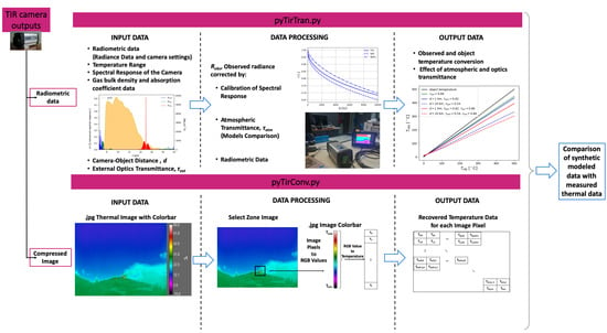
2.6. Description of Python Scripts

The PyTirCam-1.0 project was divided into the following folders:

• PyTirCam-1.0/pyTirTran: A transmission and conversion algorithm based on the spectral properties of atmospheric gases and of the TIR camera.
• PyTirCam-1.0/jpgToTIR: An algorithm based on Python PIL library to recover the radiometric thermal data from compressed images.

The two folders contain the input data, the functions defined throughout this paper, and the scripts used to retrieve the presented results, as a practical tutorial of the PyTirCam-1.0 usage.

2.6.1. PyTirCam-1.0/pyTirTran

The folder contains:

• The required input and functions to run PyTirTran.py:
  • input.py is the input file of pyTirTran.py. The required inputs are (symbols used in the script are reported in brackets): Temperature range in K (Tmin and Tmax), length of the temperature linear space (len_T), CO₂ bulk density (rhoCO2), maximum value of the camera spectral response (SpR_max), minimum and maximum wavelength of the spectral response defined as a step function (lambda_min, lambda_max), the camera-object distance (L), external optics transmittance (tauext), and the local path of the H₂O and CO₂ absorption coefficient data, beside the camera spectral response data (fileIn_*).
  • functions/__init__.py is the file containing: Fit, the function to perform curve fittings and provide optimal parameters; T_func, the function approximating $T_{IR}\left(R\right)$ as a combination of linear and power laws (see Section 2.3 and Table 1); ps, the saturation pressure of water; rhow and rhowThC, the water vapor bulk density (as in Equations (A3) and (A6), respectively); Planck and RIR, the Planck function and the Stefan-Boltzmann law corrected with the camera spectral response (Equations (1) and (5), respectively); Step, the spectral response as a step function (Section 3.1); tauA and tauThC, the atmospheric transmittances (Equations (10) and (A5), respectively); Rtot, the total radiance received by the camera sensor (Equation (16)).
• pyTirTran.py is the Python script to be executed. The script can be run to:
  • Use the spectral response of the camera or defined as step function by choosing the flag step = False or True, respectively.
  • Update the data in the folder “FigureData” the transmittance data shown in Figure 5 and Figure 6 by selecting the flag results = “tau_SR_ThC”.
  • Save the plot of the results reported and discussed in Section 3.2 (atmoAndOptics.png) and a plot showing the goodness of the approximation used in Equation (10) for the atmospheric transmittance (tauObjOnTauAtm.png), by selecting the flag results = “Figure 8”.
  • Compute and display on the terminal the data reported in

    Table 2. Settings and measurements for the hot object observations. The selected measurement scale is between 0 °C and 500 °C. $T_{flir}$, $T_{SpR}$, and $T_{ThC}$ are the observed, the theoretically corrected and the empirically corrected brightness temperatures, respectively.

    Measurement Group	${\mathit{T}}_{\mathit{a}\mathit{t}\mathit{m}}(°\mathbf{C})$	ε	${\mathit{T}}_{\mathit{r}\mathit{i}\mathit{f}\mathit{l}}(°\mathbf{C})$	d (m)	${\mathit{\omega }}_{\mathbf{\%}}$	${\mathit{T}}_{\mathit{f}\mathit{l}\mathit{i}\mathit{r}}(°\mathbf{C})$	${\mathit{T}}_{\mathit{S}\mathit{p}\mathit{R}}(°\mathbf{C})$	${\mathit{T}}_{\mathit{T}\mathit{h}\mathit{C}}(°\mathbf{C})$
    M1	20	0.98	20	3047	40%	49.7	41.6	40.0
    	40	1	40	0	0%	39.0	39.0	39.0
    	20	0.98	20	3047	40%	47.3	39.8	38.4

    ,

    Table 3. Settings and measurements for the cold object observations. The selected measurement scale is between −10 °C and 60 °C. M1, M2, M3 refer to three different points on the target object. $T_{flir}$, $T_{SpR}$, and $T_{ThC}$ are the observed, the theoretically corrected, and the empirically corrected brightness temperatures, respectively.

    Measurement Group	${\mathit{T}}_{\mathit{a}\mathit{t}\mathit{m}}(°\mathbf{C})$	ε	${\mathit{T}}_{\mathit{r}\mathit{i}\mathit{f}\mathit{l}}(°\mathbf{C})$	d (m)	${\mathit{\omega }}_{\mathbf{\%}}$	${\mathit{T}}_{\mathit{f}\mathit{l}\mathit{i}\mathit{r}}(°\mathbf{C})$	${\mathit{T}}_{\mathit{S}\mathit{p}\mathit{R}}(°\mathbf{C})$	${\mathit{T}}_{\mathit{T}\mathit{h}\mathit{C}}(°\mathbf{C})$
    M1	20	0.98	20	0	40%	−4.5	−3.94	−3.94
    	20	0.98	20	3047	40%	<−10.0	0.10	1.87
    M2	20	0.98	20	3047	40%	−6.0	2.60	4.12
    	20	0.98	20	0	40%	4.0	4.34	4.34
    M3	20	0.98	20	0	40%	4.5	4.82	4.82
    	20	0.98	20	3047	40%	−4.0	3.87	5.27

    and

    Table 4. Settings and measurements for the cold object observations. The selected measurement scale is between −10 °C and 60 °C. Each measurement group M1, M2, M3 corresponds to a different observation point. $T_{flir}$, $T_{SpR}$, and $T_{ThC}$ are the observed, the theoretically corrected, and the empirically corrected brightness temperatures, respectively.

    Measurement Group	${\mathit{T}}_{\mathit{a}\mathit{t}\mathit{m}}(°\mathbf{C})$	ε	${\mathit{T}}_{\mathit{r}\mathit{i}\mathit{f}\mathit{l}}(°\mathbf{C})$	d (m)	${\mathit{\omega }}_{\mathbf{\%}}$	${\mathit{T}}_{\mathit{f}\mathit{l}\mathit{i}\mathit{r}}(°\mathbf{C})$	${\mathit{T}}_{\mathit{S}\mathit{p}\mathit{R}}(°\mathbf{C})$	${\mathit{T}}_{\mathit{T}\mathit{h}\mathit{C}}(°\mathbf{C})$
    M1	20	0.98	20	3047	40%	−5.3	3.04	4.52
    	20	0.98	20	0	40%	4.3	4.63	4.63
    M2	20	0.98	20	0	40%	4.7	5.02	5.02
    	20	1	20	0	40%	5.0	4.99	4.99
    M3	20	0.98	20	0	40%	−0.3	0.14	0.14
    	20	0.98	20	0	0%	−0.3	0.14	0.14
    	20	0.98	20	3047	0%	−3.8	−0.47	0.12
    	20	0.98	20	3047	40%	−13	−1.73	0.22
    	20	1	20	0	40%	−0.2	−0.21	−0.21

    by choosing the flag results = “Table 2, Table 3 and Table 4”.
    • plot_technote.py is a Python script to show the plots given in Figure 5 and Figure 6.
    • FigureData is the folder containing the data of Figure 5 and Figure 6.
    • spectralData is the folder containing the HITRAN cross sections and the camera spectral response.

To use the script for different data, it is necessary to modify the input file, i.e., the path of the new spectralData folder and insert the new input values and ranges according to the new data in input.py. To add new gas components, it is sufficient to pass longer arrays to the rhoA function. In particular, the bulk density and the specific absorption coefficient data of each new gas component are needed. In addition, it is possible to obtain the results reported on Table 2, Table 3 and Table 4 for a new experiment by changing the experimental data in the corresponding part of pyTirTran.py.

2.6.2. PyTirCam-1.0/jpgToTIR

The folder contains:

• The required input and functions to run PyTirConv.py:
  • input.py is the input file of pyTirConv.py. The required inputs are the radiometric image containing the colorbar (InputImage.jpg), the bounds pixel coordinates (width “w” going left-right and height “h” going top-bottom) of both the colorbar (bar_wi, bar_wf, bar_hi, bar_hf) and the zone of the image to be analyzed (wi, wf, hi, hf), and the range of the colorbar (Tmin, Tmax).
  • InputData.dat is the file containing the source radiometric temperature data corresponding to the compressed image (InputImage.jpg). This is the file used to evaluate the accuracy of the conversion algorithm.
  • functions/__init__.py is the file containing the functions needed to retrieve the temperature data from the compressed image. The conversion can be done both with the image colorbar and the analytical colorbar. In particular, the following functions are defined: closest_color, finds the colorbar index corresponding to the closest color (by means of the Euclidean distance); analyticBar, defines a specific analytical colorbar; fromJpgToBar, finds the colorbar directly from the image; and fromJpgToArray, extract the temperature values from the compressed image.
• pyTirConv.py is the Python script to be executed. The script can be run to:
  • Covert each pixel of the selected image zone to a temperature value by finding the closest color to the RGB triplet. The temperature data and the corresponding .jpg image are saved as Temperature.dat and OutputImage.jpg, respectively. By choosing the flag load = True, it is possible to run the part of the script related only to the data analysis by loading the previously recovered temperature data beside their corresponding image.
  • Save an image (difference.jpg) showing the difference between the colors of the input image (InputImage.jpg) and those of the recovered one (OutputImage.jpg), by selecting the flag evalConv = True.
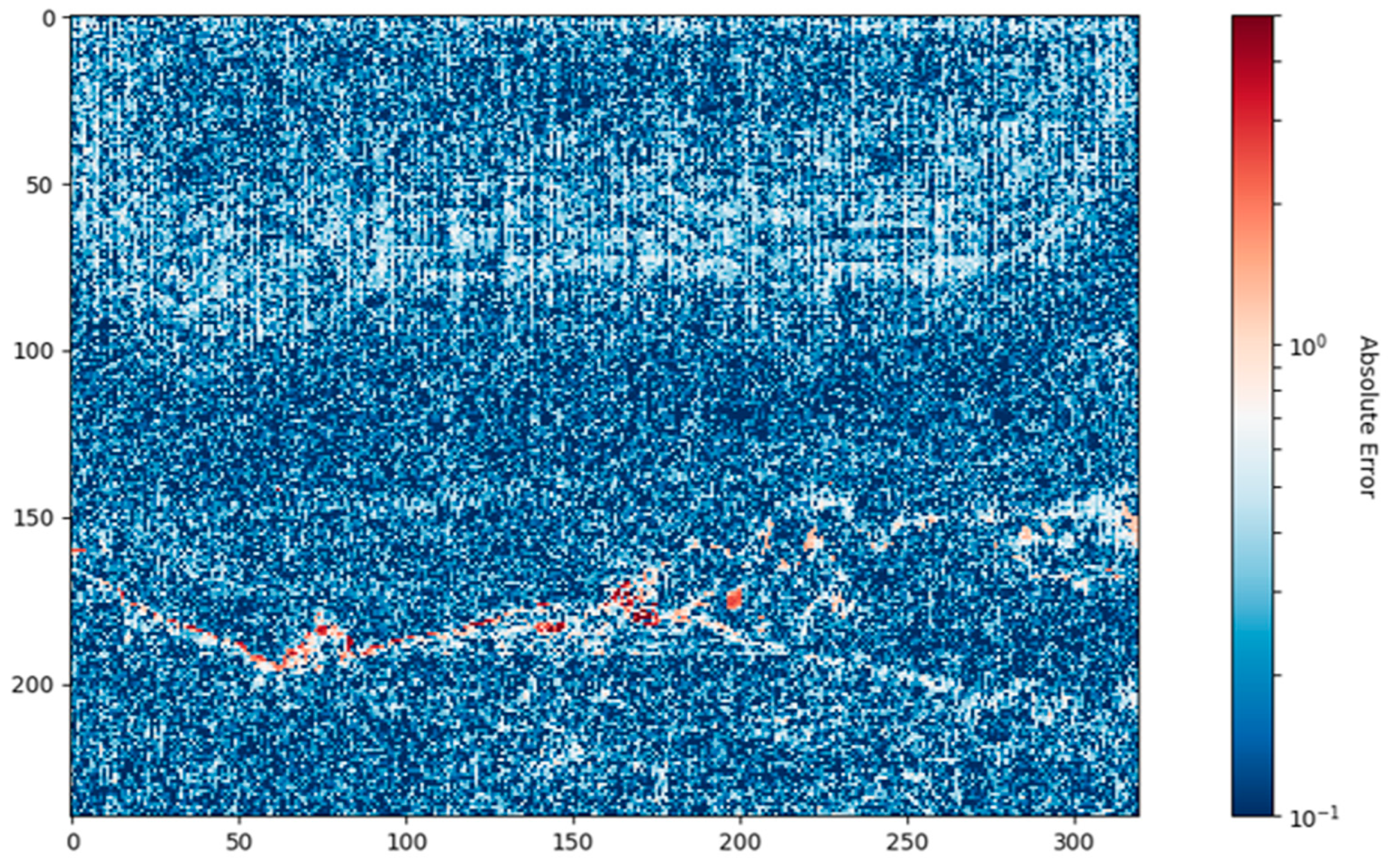
  • Compute the absolute error between the radiometric (InputData.dat) and the recovered data (Temperature.dat) by selecting the flag evalRadio = True. Moreover, this flag prints the maximum, average, and minimum temperature error.
  • Do the above operations (1–3), also with the analytical colorbar, by choosing the flag analytic = True. This flag shows also the comparison of the two colorbars.
• Output files: The recovered temperature data and image from both the image and analytic colorbars (Temperature.dat, Temperature_analytic.dat, OutputImage.jpg, OutputImage_analytic.jpg) and the difference between the radiometric and recovered data using both colorbars (difference.jpg, difference_analytic.jpg).

It is possible to apply the script for other images by modifying the input.py file according to the new image coordinates. It is worth nothing that the script can be applied to any 2D colormap when the variable showed is quantified with a colorbar.

3. Results and Discussion

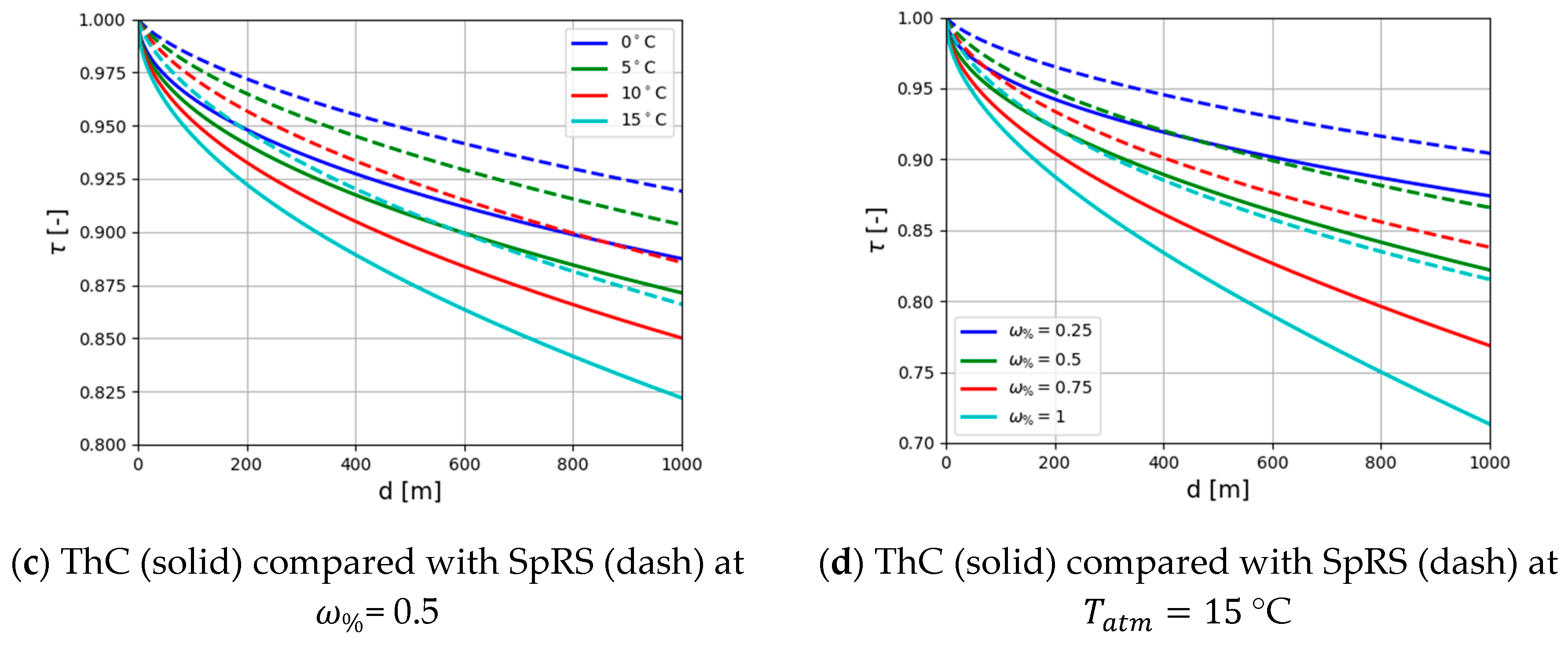
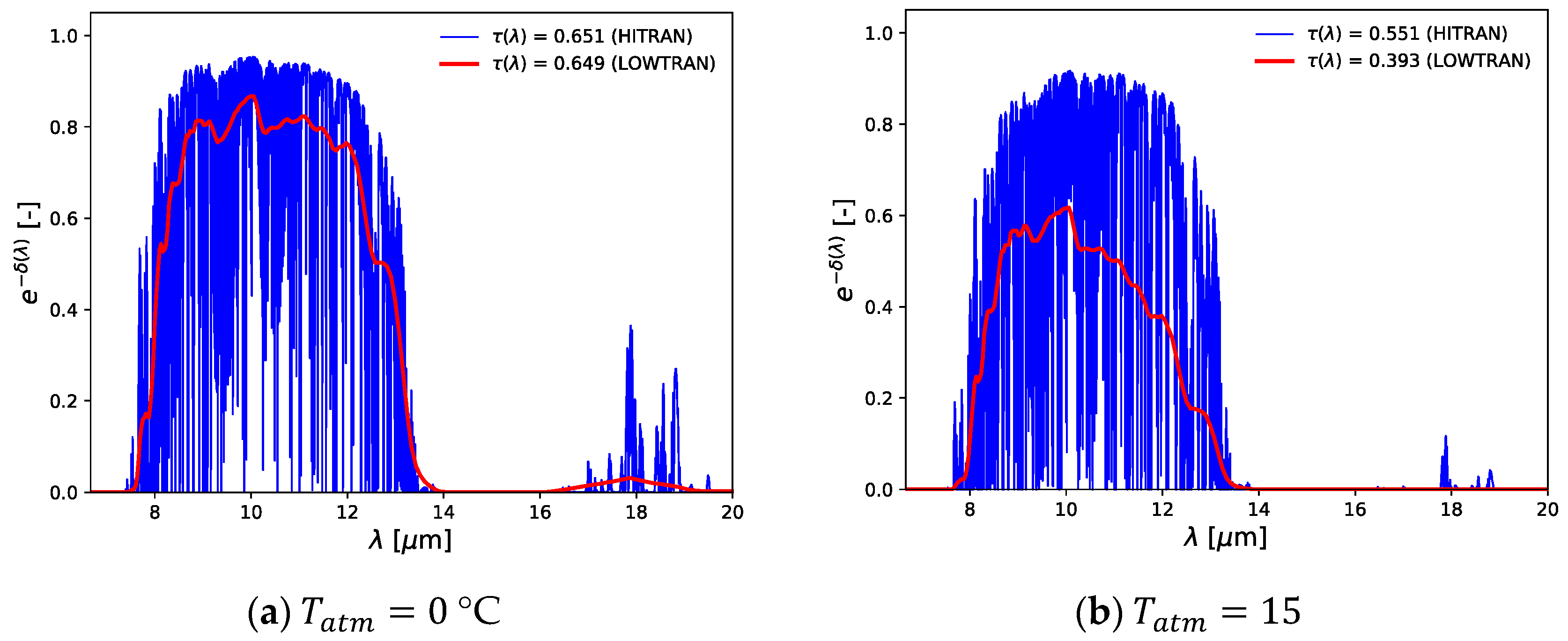
3.1. Atmospheric Transmittance Models Comparison

The method used to describe atmospheric transmission can significantly affect the thermal measurements. Significantly different atmospheric transmittance coefficients can be obtained in the LWIR band by changing the algorithm used by TIR cameras, using different transmission models, or empirical tables [31].

We compared the expression of the transmittance given by Equation (10) and that used by FLIR for ThermaCAM-PM-595-LW in the wavelength window [7.5, 13] µm, described by the authors of [31] (see Equation (A5), Appendix B). Equation (10) was calculated using $sr\left(\lambda \right),$ either as in Figure 1a or as a step function defined as equal to 1 for $\lambda \in \left[7.5,13\right]\mathsf{\mu }\mathrm{m}$ and 0 elsewhere. We refer to the model used by ThermaCAM-PM-595-LW as ThC, to Equation (10) with $sr\left(\lambda \right)$ of Figure 1a as SpR, and to Equation (10) with a step function as SpRS. Figure 5 compares SpR and SpRS with ThC at short distances ($d<1$ km). It shows the atmospheric transmittance with respect to the camera-to-object distance as a function of $T_{atm}$, with relative humidity ${\omega }_{\%}$ = 0.5; and as a function of ${\omega }_{\%}$ with $T_{atm}=15$ °C. Figure 6 shows the atmospheric transmission up to 10 km for the cases ${\omega }_{\%}$ = 0.5 and $T_{atm}$ = 0, 15 °C, obtained with ThC, SpR and SpRS. Data can be reproduced using pyTirTran.

As shown by the authors of [31], we obtained a wide variability of the transmission coefficients depending on the adopted model. At short distances, SpR provided smaller transmittances than ThC when ${\omega }_{\%}\le 0.5$. On the other hand, SpR absorbed less than ThC when ${\omega }_{\%}>0.5$. It is worth noting that SpR and ThC gave similar results in the case ${\omega }_{\%}$ = 0.5 and $T_{atm}$ = 15 °C. At long distances, SpR absorbed more than ThC in cold conditions (Figure 6a), but it did the opposite when $T_{atm}$ = 15 °C (Figure 6b). SpRS absorbed always less than ThC.

This comparison shows how the atmospheric transmittance is sensitive to the spectral response of the camera. At short distances, SpR behaved much similarly to ThC than SpRS did. Moreover, ThC was somehow between SpR and SpRS. We can thus conclude that, at short distances, the spectral response used in Equation (10) can have a significant role in determining the discrepancies between ThC and SpR obtained in this and in the previous subsection. On the other hand, the fact that the maximum allowed distance in the camera settings is 3 km may indicate that ThC cannot be safely used at greater distances. Unfortunately, we cannot directly evaluate the accuracy of either ThC or SpR transmission models because they strongly depend not only on the optical properties of the atmosphere, but also on the particular spectral response of the camera. In Section 3.3, we analyze a simple experiment to directly test the TIR camera measurements.

At distance $d=10$ km, the above results were compared with LOWTRAN, a Low-Resolution Transmittance open-source code [45,46], to provide further comparison with a widely used atmospheric transmittance model. The code enables the evaluation of the spectral transmittance of a horizonal portion of atmosphere. Setting the same compositions and parameters used in this section, we obtained the results reported in Figure 7.

Whereas the comparison of LOWTRAN with the high-resolution HITRAN spectral transmittance that we used in SpR was very good at 0 °C, the atmospheric transmittance calculated with the former model was smaller at 15 °C. The main sources of discrepancy were the spectral resolution and water self-line-broadening [60]. The latter effect was small to negligible except for water vapor at bottom of the Earth’s atmosphere [44]. In this case, to provide agreement with experimental results, the water vapor continuum has been formulated in literature by empirically broadening the collisional Lorentz shape of water absorption lines [61]. This effect can be considered in pyTirTran by substituting the HITRAN water cross section with the smoother water continuum. This functionality will be provided in future developments.

3.2. Effect of the Atmospheric and External Optics Corrections on High Temperature Measurements

Here, we want to show how the atmospheric and external optics corrections affect the brightness temperature data as the contrast between the object and the atmospheric temperature changes. In Figure 8, we show each of these effects, when an object with $ϵ=0.98$ was at 1 km and 10 km of distance, in an atmosphere at 20 °C with 40% relative humidity, and ${\tau }_{ext}=0.86$. Since Equation (16) is linear with respect to radiances, the relationship between $T_{obj}$ and $T_{obs}$ is quasilinear, and we can focus on the maximum temperature contrast ($T_{obj}=500$ °C) to highlight the weight of each effect. In the case defined above, the effect of the external optics is comparable with the effect of 1 km of atmosphere because ${\tau }_{atm}=0.82$. In particular, when $T_{obj}=500$ °C, we obtained $T_{obs}=$ 447 °C and 435 °C, respectively. Combining the two effects at 1 km of distance, we obtained $T_{obs}=395$ °C. Moving to 10 km of distance, the increasing atmospheric optical thickness led to ${\tau }_{atm}=0.54$, corresponding to $T_{obs}=303$ °C and 333 °C, respectively, with and without external optics. These numbers quantified the influence of the two main effects affecting the observed brightness temperature, highlighting the crucial importance of the correction algorithms needed to retrieve the object temperature.

It is worth noting that, in practical monitoring applications, external optics are subject to corrosion due to atmospheric particulate, aerosols, and some gases, such as CO₂, SO₂, HCl, and HF. This aspect is particularly critical in the monitoring of volcanoes, which also have the presence of ash and sulfur. In the worst cases, it is necessary to replace the external optics every few months. The degradation of the transmission coefficient over time will be investigated in future studies.

3.3. Comparison between Experimental Data and Theoretical Atmospheric Correction

In this section, we experimentally checked how the camera settings influenced the acquired brightness temperature of an object kept at an approximately constant temperature and position with respect to the camera. We changed the following setting parameters: Distance 0 m or 3047 m; relative humidity 0% or 40%; emissivity 0.98 or 1; atmospheric and reflected temperature 20 °C or 40 °C. The results are reported in Table 2, Table 3 and Table 4. There, $T_{flir}$ was the temperature given by the camera; $T_{SpR}$ was the temperature corrected using Equations (9), (10), and (16); and $T_{ThC}$ was the temperature corrected using the empirical algorithm ThC in Equation (A5). When $d=0$ and $ϵ=1$, we should have had $\tau =1$ and $T_{SpR}=T_{flir}$. When $d>0$ or $ϵ<1$ in the camera settings, the measured temperature $T_{flir}$ changed. Our aim was to verify that $T_{SpR}$ was approximately not influenced by the camera settings, meaning that our theoretical atmospheric correction worked similarly to that implemented in the device.

The thermal data measured on the hot object showed that $T_{flir}$ varied from 48.5 °C to 39 °C when $d$ moved from 3047 m to 0 m (see Table 2 for more details). $T_{flir}>T_{SpR}$ when $d>0$ because the camera was trying to correct for the presence of approximately 3 km of colder atmosphere. Our theoretical atmospheric correction kept $T_{SpR}=40.1$ ± 1.1 °C, while the camera algorithm gave $T_{ThC}=39.1$ ± 0.7 °C.

In Table 3, the measurements on the cold object were performed by changing the sole parameter $d$. They were divided in three groups: M1, M2, and M3. Similar to the hot object observations, a variation in the TIR measurements was obtained by changing $d$ from 0 m to 3047 m and by keeping the other parameters constant. In this case, we obtained $T_{SpR}=-1.9\pm 2.0,3.5\pm 0.9,4.3\pm 0.5$ °C, respectively, for M1, M2, and M3. The camera algorithm gave $T_{ThC}=-1.0\pm 2.9,4.2\pm 0.1,5.0\pm 0.2$ °C, respectively. The first group showed a larger error because its second measurement was off-range.

In Table 4, the measurements on the cold object were performed using different combinations of the parameters $T_{atm}$, ε, $T_{rifl}$, d, ${\omega }_{\%}$, and external optics. In this case, we obtained $T_{SpR}=3.8\pm 0.8,5.0\pm 0.1,-0.4\pm 0.7$ °C, respectively, for M1, M2, and M3. The camera algorithm gave $T_{ThC}=4.6\pm 0.1,5.0\pm 0.1,0.1\pm 0.1$ °C, respectively.

We verified that our theoretical atmospheric correction is able to keep $T_{SpR}$ constant within an error of 1.1 °C. We verified also that the empirical atmospheric correction, Equation (A5), keeps $T_{ThC}$ constant within an error of 0.7 °C.

In our simple experiment, the algorithm ThC worked as expected and could be used to understand how the camera atmospheric correction works. However, the algorithm used by the camera was empirical, implicitly depended on the particular camera spectral response, and has been tested only up to 3 km. For these reasons, we also tested a theoretical atmospheric correction based directly on the specific spectral absorption coefficients of air and water. We found that this algorithm worked coherently to that implemented in the camera with a slight increase in the relative error. This fact does not necessarily mean that the empirical algorithm computed the atmospheric transmission coefficient in a more accurate way. Instead, we can only conclude that the camera actually used an algorithm that was more similar (if not exactly the same) to the empirical one. Both the theoretical and empirical algorithms behaved similarly within an error of approximately 1 °C.

3.4. Brightness Temperature from a .jpg Image Acquired on 16 November 2006

We used the radiometric data corresponding to the .jpg image given in Figure 4 to estimate the error in the procedure described in Section 2.5. In other words, we compared the temperature matrix effectively measured by the camera with the temperature reconstructed from the .jpg image. Figure 9 shows the absolute deviation between the measured and recovered data. In the plume and in the atmosphere, we mainly obtained an absolute error smaller than 2 °C, while the maximum discrepancy was limited to the high-contrast temperature zones along the volcano-atmosphere edges. In the latter regions, the image quality was affected by the simultaneous presence of atmosphere, soil, and volcanic plume, leading to a greater error in the recorded thermal image and, consequently, in the reconstructed data.

The comparison between the measured and recovered data shows that the algorithm described in Section 2.5 and implemented in pyTirConv can retrieve temperature data from .jpg images with relatively good accuracy when used far from high-contrast zones.

4. Conclusions

The aim of this work was twofold: (a) To understand and manage how the camera settings influence the radiance and brightness temperature measurements, and (b) to process and recover the temperature data measured and recorded as .jpg images. The package PyTirCam, containing a couple of Python scripts (pyTirTran and pyTirConv), was developed to deal with these two objectives. The first considers atmospheric absorption and emission beside object emissivity and reflectivity. The atmospheric transmission coefficient was implemented using two methodologies: (1) A transmission model based directly on the spectral infrared absorption coefficients of atmospheric components (extracted from the HITRAN database) combined with the camera spectral response (in the paper, we referred to it as SpR); (2) the empirical algorithm implemented into the commercial camera used in this work (in the paper, we referred to it as ThC). The first method can be generalized to any camera, given its spectral response, and to any atmosphere, given its composition. The second one was empirically calibrated with the particular type of camera used in this work. In addition, the algorithm estimates the effective transmittance of the external optics, taking into account the particular spectral properties of the camera and of the optics themselves. This script allows the user to quantify each of the approximations discussed in the paper.

A simple experiment was presented to verify, within an error of approximately 1 °C, that: (1) The empirical algorithm ThC was actually the one used by the camera; (2) our atmospheric transmission model, SpR, gives results similar to those obtained with ThC; (3) the maximum spectral response of the camera can be derived from camera radiometric data; (4) the conversion from radiance to brightness temperature used by the camera can be recovered theoretically from its spectral response. Our results showed that the atmospheric and external optics transmittances were strongly related to the camera spectral response and, as a consequence, were affected by the camera particular conditions.

We identified and quantified the main approximations used by the camera software: (1) The empirical algorithm for the atmospheric transmission coefficient was calibrated up to 3 km; (2) the atmospheric transmission coefficient was always calculated using the atmospheric temperature, while, in principle, it should consider the object temperature in the absorption term (${\tau }_{obj}\approx {\tau }_{atm}$); (3) the emissivity and reflectivity coefficients were considered constants; (4) the atmospheric composition was fixed and could not be changed; (5) the atmosphere was considered to be at a constant temperature. Even if the camera algorithm did not perfectly reproduce the atmospheric transmittance, it was the algorithm used by the camera to recover the object temperature from the observed object. Thus, it was the algorithm used to recover the unprocessed data. We need camera algorithms when the camera settings are different from the real monitoring conditions or when we want to use a different atmospheric transmission model. In volcanic monitoring, this situation is very likely to happen, e.g., the ENT camera, which uses fixed setting parameters, was installed in proximity of Mt. Etna volcano at an altitude of $~700$ m a.s.l. and a distance of $~15$ km from the volcanic craters, with weather conditions that changed day by day and typically also during the same day. In this case, we needed to filter out any setting correction to recover the actual radiance impacting the camera.

To overcome the problem of data storage capabilities, some of the volcanic surveillance systems can keep only compressed .jpg thermal images. For this reason, the second algorithm, pyTirConv, was developed to recover the radiometric data from TIR .jpg images. In the plume and atmosphere pixels, the temperature data were recovered within an error of 2 °C, i.e., in zones of the image that were far from the volcano edges and without strong temperature discontinuities.

Our results provide methods to better understand the thermal data collected by volcano surveillance systems, furnishing technical procedures to use them quantitatively. The procedures presented in this work are general and can be applied to different TIR cameras installed both at ground and airborne platforms. Future developments include the integration of the described algorithms in existing automated procedures to analyze thermal infrared scenes acquired by permanent ground-based or satellite surveillance systems.

References

1. Flynn, L.P.; Mouginis-Mark, P.J.; Gradie, J.C.; Lucey, P.G. Radiative temperature measurements at Kupaianaha Lava Lake, Kilauea Volcano, Hawaii. J. Geophys. Res. Solid Earth 1993, 98, 6461–6476. [Google Scholar] [CrossRef]
2. Pinkerton, H.; James, M.; Jones, A. Surface temperature measurements of active lava flows on Kilauea volcano, Hawai’i. J. Volcanol. Geotherm. Res. 2002, 113, 159–176. [Google Scholar] [CrossRef] [Green Version]
3. Calvari, S.; Pinkerton, H. Birth, growth and morphologic evolution of the “Laghetto” cinder cone during the 2001 Etna eruption. J. Volcanol. Geotherm. Res. 2004, 132, 225–239. [Google Scholar] [CrossRef]
4. Calvari, S.; Spampinato, L.; Lodato, L.; Harris, A.J.L.; Patrick, M.R.; Dehn, J.; Burton, M.R.; Andronico, D. Chronology and complex volcanic processes during the 2002-2003 flank eruption at Stromboli volcano (Italy) reconstructed from direct observations and surveys with a handheld thermal camera. J. Geophys. Res. Solid Earth 2005, 110. [Google Scholar] [CrossRef] [Green Version]
5. Harris, A. Thermal Remote Sensing of Active Volcanoes: A User’s Manual; Cambridge University Press: Cambridge, UK, 2011. [Google Scholar]
6. Platt, U.; Bobrowski, N.; Butz, A. Ground-Based Remote Sensing and Imaging of Volcanic Gases and Quantitative Determination of Multi-Species Emission Fluxes. Geosciences 2018, 8, 44. [Google Scholar] [CrossRef] [Green Version]
7. Prata, F.J.; Bernardo, C. Retrieval of volcanic ash particle size, mass and optical depth from a ground-based thermal infrared camera. J. Volcanol. Geotherm. Res. 2009, 186, 91–107. [Google Scholar] [CrossRef]
8. Prata, F.J.; Bernardo, C. Retrieval of sulphur dioxide from a ground-based thermal infrared imaging camera. Atmos. Meas. Tech. Discuss. 2014, 7, 1153–1211. [Google Scholar] [CrossRef]
9. Harris, A.J.L.; Ripepe, M. Temperature and dynamics of degassing at Stromboli. J. Geophys. Res. 2007, 112, B03205. [Google Scholar] [CrossRef]
10. Blackett, M. An Overview of Infrared Remote Sensing of Volcanic Activity. J. Imaging 2017, 3, 13. [Google Scholar] [CrossRef]
11. Coppola, D.; Laiolo, M.; Cigolini, C.; Massimetti, F.; Delle Donne, D.; Ripepe, M.; Arias, H.; Barsotti, S.; Parra, C.B.; Centeno, R.G.; et al. Thermal Remote Sensing for Global Volcano Monitoring: Experiences From the MIROVA System. Front. Earth Sci. 2020, 7, 362. [Google Scholar] [CrossRef] [Green Version]
12. Spampinato, L.; Calvari, S.; Oppenheimer, C.; Boschi, E. Volcano surveillance using infrared cameras. Earth Sci. Rev. 2011, 106, 63–91. [Google Scholar] [CrossRef]
13. Calvari, S.; Lodato, L.; Steffke, A.; Cristaldi, A.; Harris, A.J.L.; Spampinato, L.; Boschi, E. The 2007 stromboli eruption: Event chronology and effusion rates using thermal infrared data. J. Geophys. Res. Solid Earth 2010, 115, 1–20. [Google Scholar] [CrossRef] [Green Version]
14. Andronico, D.; Taddeucci, J.; Cristaldi, A.; Miraglia, L.; Scarlato, P.; Gaeta, M. The 15 March 2007 paroxysm of Stromboli: Video-image analysis, and textural and compositional features of the erupted deposit. Bull. Volcanol. 2013, 75, 733. [Google Scholar] [CrossRef]
15. Tran, Q.H.; Han, D.; Kang, C.; Haldar, A.; Huh, J. Effects of Ambient Temperature and Relative Humidity on Subsurface Defect Detection in Concrete Structures by Active Thermal Imaging. Sensors 2017, 17, 1718. [Google Scholar] [CrossRef]
16. Weng, Q. Thermal infrared remote sensing for urban climate and environmental studies: Methods, applications, and trends. ISPRS J. Photogramm. Remote Sens. 2009, 64, 335–344. [Google Scholar] [CrossRef]
17. Menzel, W.P.; Tobin, D.C.; Revercomb, H.E. Infrared Remote Sensing with Meteorological Satellites. Adv. At. Mol. Opt. Phys. 2016, 65, 193–264. [Google Scholar] [CrossRef]
18. Du, X.; Cao, D.; Mishra, D.; Bernardes, S.; Jordan, T.R.; Madden, M. Self-adaptive gradient-based thresholding method for coal fire detection using ASTER thermal infrared data, Part I: Methodology and decadal change detection. Remote Sens. 2015, 7, 6576–6610. [Google Scholar] [CrossRef] [Green Version]
19. Ren, H.; Du, C.; Liu, R.; Qin, Q.; Meng, J.; Li, Z.L.; Yan, G. Evaluation of radiometric performance for the Thermal Infrared Sensor onboard Landsat 8. Remote Sens. 2014, 6, 12776–12788. [Google Scholar] [CrossRef] [Green Version]
20. Pfeffer, M.A.; Bergsson, B.; Barsotti, S.; Stefánsdóttir, G.; Galle, B.; Arellano, S.; Conde, V.; Donovan, A.; Ilyinskaya, E.; Burton, M.; et al. Ground-Based measurements of the 2014-2015 holuhraun volcanic cloud (Iceland). Geosciences 2018, 8, 29. [Google Scholar] [CrossRef] [Green Version]
21. Andò, B.; Pecora, E. An advanced video-based system for monitoring active volcanoes. Comput. Geosci. 2006, 32, 85–91. [Google Scholar] [CrossRef]
22. Corradino, C.; Ganci, G.; Cappello, A.; Bilotta, G.; Calvari, S.; Negro, C.D. Recognizing eruptions of Mount Etna through machine learning using multiperspective infrared images. Remote Sens. 2020, 12, 970. [Google Scholar] [CrossRef] [Green Version]
23. Cerminara, M.; Esposti Ongaro, T.; Valade, S.; Harris, A.J.L. Volcanic plume vent conditions retrieved from infrared images: A forward and inverse modeling approach. J. Volcanol. Geotherm. Res. 2015, 300, 129–147. [Google Scholar] [CrossRef] [Green Version]
24. Valade, S.; Harris, A.J.L.; Cerminara, M. Plume Ascent Tracker: Interactive Matlab software for analysis of ascending plumes in image data. Comput. Geosci. 2014, 66, 132–144. [Google Scholar] [CrossRef]
25. Sansivero, F.; Scarpato, G.; Vilardo, G. The automated infrared thermal imaging system for the continuous long-term monitoring of the surface temperature of the Vesuvius crater. Ann. Geophys. 2013, 56, S0454. [Google Scholar] [CrossRef]
26. Sansivero, F.; Vilardo, G. Processing thermal infrared imagery time-series from volcano permanent ground-based monitoring network. Latest methodological improvements to characterize surface temperatures behavior of thermal anomaly areas. Remote Sens. 2019, 11, 553. [Google Scholar] [CrossRef] [Green Version]
27. Russo, G.; Reitano, D.; Pecora, E.; Biale, E. Thermal Camera Data Tool (T.C.D.) per L’Analisi Dei Dati da Telecamera Termica. Rapporti Tecnici INGV 2008, 84. Available online: http://hdl.handle.net/2122/4652 (accessed on 5 December 2020).
28. Gaudin, D.; Taddeucci, J.; Scarlato, P.; Harris, A.J.L.; Bombrun, M.; Del Bello, E.; Ricci, T. Characteristics of puffing activity revealed by ground-based, thermal infrared imaging: The example of Stromboli Volcano (Italy). Bull. Volcanol. 2017, 79, 24. [Google Scholar] [CrossRef]
29. Labazuy, P.; Gouhier, M.; Harris, A.; Guéhenneux, Y.; Hervo, M.; Bergès, J.C.; Fréville, P.; Cacault, P.; Rivet, S. Near real-time monitoring of the April-May 2010 Eyjafjallajökull ash cloud: An example of a web-based, satellite data-driven, reporting system. Int. J. Environ. Pollut. 2012, 48, 262–272. [Google Scholar] [CrossRef]
30. Wright, R.; Flynn, L.; Garbeil, H.; Harris, A.; Pilger, E. Automated volcanic eruption detection using MODIS. Remote Sens. Environ. 2002, 82, 135–155. [Google Scholar] [CrossRef] [Green Version]
31. Minkina, W.; Klecha, D. Atmospheric transmission coefficient modelling in the infrared for thermovision measurements. J. Sens. Sens. Syst. 2016, 5, 17–23. [Google Scholar] [CrossRef] [Green Version]
32. Minkina, W.; Klecha, D. Modeling of Atmospheric Transmission Coefficient in Infrared for Thermovision Measurements. In Proceedings of the AMA Conferences 2015, Nürnberg, Germany, 19–21 May 2015; pp. 903–907. [Google Scholar] [CrossRef]
33. Ball, M.; Pinkerton, H. Factors affecting the accuracy of thermal imaging cameras in volcanology Factors affecting the accuracy of thermal imaging cameras in volcanology. J. Geophys. Res. Solid Earth 2006. [Google Scholar] [CrossRef]
34. Sawyer, G.M.; Burton, M.R. Effects of a volcanic plume on thermal imaging data. Geophys. Res. Lett. 2006, 33, L14311. [Google Scholar] [CrossRef]
35. HITRANonline. Available online: http://hitran.org/ (accessed on 6 November 2020).
36. Wilkes, T.C.; Stanger, L.R.; Willmott, J.R.; Pering, T.D.; McGonigle, A.J.S.; England, R.A. The development of a low-cost, near infrared, high-temperature thermal imaging system and its application to the retrieval of accurate lava lake temperatures at Masaya volcano, Nicaragua. Remote Sens. 2018, 10, 450. [Google Scholar] [CrossRef] [Green Version]
37. Bonadonna, C.; Folch, A.; Loughlin, S.; Puempel, H. Future developments in modelling and monitoring of volcanic ash clouds: Outcomes from the first IAVCEI-WMO workshop on Ash Dispersal Forecast and Civil Aviation. Bull. Volcanol. 2012, 74, 1–10. [Google Scholar] [CrossRef] [Green Version]
38. Bonadonna, C.; Costa, A. Modeling tephra sedimentation from volcanic plumes. In Modeling Volcanic Processes: The Physics and Mathematics of Volcanism; Cambridge University Press: Cambridge, UK, 2013; pp. 173–202. [Google Scholar]
39. Costa, A.; Macedonio, G.; Folch, A. A three-dimensional Eulerian model for transport and deposition of volcanic ashes. Earth Planet. Sci. Lett. 2006, 241, 634–647. [Google Scholar] [CrossRef]
40. Folch, A.; Costa, A.; Macedonio, G. FALL3D: A computational model for transport and deposition of volcanic ash. Comput. Geosci. 2009, 35, 1334–1342. [Google Scholar] [CrossRef]
41. Zehner, C. Monitoring Volcanic Ash From Space. In Proceedings of the ESA-EUMETSAT Workshop on the 14 April to 23 May 2010 Eruption at the Eyjafjöll Volcano, South Iceland, Frascati, Italy, 26–27 May 2010; Zehner, C., Ed.; ESA: Frascati, Italy, 2012. [Google Scholar]
42. Rothman, L.S.; Gordon, I.E.; Babikov, Y.; Barbe, A.; Benner, D.C.; Bernath, P.F.; Birk, M.; Bizzocchi, L.; Boudon, V.; Brown, L.R.; et al. The HITRAN2012 molecular spectroscopic database. J. Quant. Spectrosc. Radiat. Transf. 2013, 130, 4–50. [Google Scholar] [CrossRef]
43. How to Calculate Absorption Coefficient (or Absorbance) from HITRAN Data. Available online: http://home.pcisys.net/~bestwork.1/CalcAbs/CalcAbsHitran.html (accessed on 8 November 2020).
44. Schreier, F.; Gimeno García, S.; Hochstaffl, P.; Städt, S. Py4CAtS—PYthon for Computational ATmospheric Spectroscopy. Atmosphere 2019, 10, 262. [Google Scholar] [CrossRef] [Green Version]
45. Kneizys, F.X.; Shettle, E.; Abreu, L.W.; Chetwynd, J.H.; Anderson, G.P. User guide to LOWTRAN 7. Environ. Res. Pap. 1988, 1010, 1–137. [Google Scholar]
46. Hirsch, M. LOWTRAN: Python Module for Atmospheric Absorption Modeling. Available online: https://zenodo.org/record/213475/export/xd#.X84WOrOxVPY (accessed on 5 December 2020).
47. Pecora, E.; Biale, E. Applicazioni delle telecamere termiche Flir A 40 M e Flir 320 M al monitoraggio di Stromboli e dell’Etna. Report INGV 2004. Prot. int. n° UFVG2004/036. Available online: http://hdl.handle.net/2122/10088 (accessed on 5 December 2020).
48. Pecora, E.; Biale, E.; Reitano, D. Evoluzione E Sviluppo Della Rete Permanente di Telecamere Fisse per Il Monitoraggio Video Dell’Etna. Rapporti Tecnici INGV 2006, 32. Available online: http://hdl.handle.net/2122/4663 (accessed on 5 December 2020).
49. Video Sorveglianza Vulcanica Etna. Available online: http://www.ct.ingv.it/index.php/monitoraggio-e-sorveglianza/segnali-in-tempo-reale/video-sorveglianza-vulcanica-etna (accessed on 3 November 2020).
50. Andronico, D.; Spinetti, C.; Cristaldi, A.; Buongiorno, M.F. Observations of Mt. Etna volcanic ash plumes in 2006: An integrated approach from ground-based and polar satellite NOAA-AVHRR monitoring system. J. Volcanol. Geotherm. Res. 2009, 180, 135–147. [Google Scholar] [CrossRef]
51. Andronico, D.; Scollo, S.; Cristaldi, A.; Ferrari, F. Monitoring ash emission episodes at Mt. Etna: The 16 November 2006 case study. J. Volcanol. Geotherm. Res. 2009, 180, 123–134. [Google Scholar] [CrossRef]
52. FLIR Systems, Inc. User’s Manual FLIR Tools/Tools+ 5.1; FLIR: Wilsonville, OR, USA, 2015; p. T810209. Available online: http://91.143.108.245/Downloads/Flir/Dokumentation/t810209-en-us_a4.pdf (accessed on 5 December 2020).
53. FLIR Systems, Inc. ResearchIR 4 User’s Guide; FLIR: Wilsonville, OR, USA, 2015; p. 29354-000. Available online: https://assets.tequipment.net/assets/1/26/FLIR_ResearchIR_User_Manual.pdf (accessed on 5 December 2020).
54. CorDEX Instruments. Ir Window Transmission Guide Book; CorDEX Instruments Ltd.: Houston, TX, USA, ID 4015 Rev A; Available online: http://www.grupoalava.com/repositorio/97d2/pdf/5436/2/cordex-instruments----ir-window-transmission-guidebook.pdf?d=1 (accessed on 5 December 2020).
55. Holliday, T.; Kay, J.A. Inaccuracies introduced using infrared windows and cameras. In IEEE Petroleum and Chemical Industry Technical Conference (PCIC); IEEE: San Francisco, CA, USA, 2014; pp. 53–59. [Google Scholar] [CrossRef]
56. Danjoux, B.R. Window and External Optics Transmittance Window and External Optics Transmittance. Flir Syst. Infrared Train. Cent. Tech. Pub. 2012, 60, 1–9. [Google Scholar]
57. Madding, R.P. Infrared Window Transmittance Temperature Dependence. Flir Syst. Infrared Train. Cent. InfraMation 2004, 104, 1–10. [Google Scholar]
58. EOT-Start Page. Available online: http://www.eot.it/ (accessed on 3 November 2020).
59. Clark, A. Pillow (PIL Fork). 2020. Available online: http://www.10.5281/zenodo.4118627 (accessed on 5 December 2020).
60. Clough, S.A.; Kneizys, F.X.; Davies, R.W. Line shape and the water vapor continuum. Atmos. Res. 1989, 23, 229–241. [Google Scholar] [CrossRef]
61. Mlawer, E.J.; Payne, V.H.; Moncet, J.L.; Delamere, J.S.; Alvarado, M.J.; Tobin, D.C. Development and recent evaluation of the MT-CKD model of continuum absorption. Philos. Trans. R. Soc. A Math. Phys. Eng. Sci. 2012, 370, 2520–2556. [Google Scholar] [CrossRef] [Green Version]
Figure 1. (a) Spectral response function of the FLIR camera as used throughout this paper. Its maximum value has been fixed to 0.82 (see Section 2.3); (b) radiance emitted from a blackbody R B B ( T ) and received by the TIR camera R I R ( T ) , as a function of temperature T .
Remotesensing 12 04056 g001
Figure 2. (a) Spectral transmittance, s t ( λ ) , of a Ge window used by INGV-OE beside the spectral response of the camera combined with the external optics s t ( λ ) s r ( λ ) ; (b) External optics transmittance as ratio of the radiance received by the TIR camera with and without external optics: R I R ( T ) , and R I R ( T ) , respectively.
Remotesensing 12 04056 g002
Figure 3. (a) Setup used to take thermal measurements by means of a FLIR A40 M camera. The keyboard on the TIR camera enables the setting changes. (b) The monitor shows the setting parameters used at Nicolosi. The brightness temperature range is between 0 °C and 500 °C, while the display scale is between −10 °C and 60 °C. The cross with label 1 represents the target point.
Remotesensing 12 04056 g003
Figure 4. Exported Mt. Etna image in .jpg format by means of ResearchIR software in the temperature range of [−10, 60] °C. The frame captures an instant of the 16 November 2006 paroxysmal episode at the South East Crater (SEC), showing: (i) The explosive activity above the crater forming the volcanic plume directed to the NE; (ii) effusive activity at the base of SEC (white arrow/glowing spot on the right); (iii) the fissure opened on the flank of the Bocca Nuova crater (BN; yellow arrow/glowing dot on the left).
Remotesensing 12 04056 g004
Figure 5. Short distance ( d < 1 km) atmospheric transmittance calculated according to the ThermaCAM-PM-595-LW algorithm (ThC) compared with Equation (10) using: (a,b) FLIR typical spectral response (SpR); (c,d) step function spectral response for λ [ 7.5 , 13 ] μm (SpRS).
Remotesensing 12 04056 g005aRemotesensing 12 04056 g005b
Figure 6. Long distance ( d < 10 km) atmospheric transmittance calculated according to the ThermaCAM-PM-595-LW algorithm (ThC, solid) compared with Equation (10) using FLIR typical spectral response (SpR, dash) or step function spectral response for λ [ 7.5 , 13 ] μm (SpRS, point-dash) at humidity ω % = 0.5 .
Remotesensing 12 04056 g006
Figure 7. Long distance ( d = 10 km) atmospheric spectral transmittance τ ( λ ) = e δ ( λ ) d , calculated at humidity ω % = 0.5 with LOWTRAN (red) and with Equation (7) (blue). The transmittances given in legend were calculated using FLIR typical spectral response (SpR, Equation (10)).
Remotesensing 12 04056 g007
Figure 8. Variation of the observed temperature, T o b s , due to the presence of atmosphere (blue), external optics (green), and both effects (red). Here, Equation (16) is used to represent T o b s as a function of the object temperature, T o b j , at 1 km (solid) and 10 km (dashed) of distance. The object temperature (black) is reported as a reference.
Remotesensing 12 04056 g008
Figure 9. Absolute error between temperature data measured by the camera and those obtained using the conversion procedure described in Section 2.5 and implemented in pyTirConv.
Remotesensing 12 04056 g009