The Role of Mean Sea Level Annual Cycle on Extreme Water Levels Along European Coastline


Abstract
:
1. Introduction
2. Datasets and Methodology
2.1. Sea Level Datatasets
2.2. Storm Impact Database
- Pan-European HANZE database [8] from 1870 to 2016: 1564 flooding events were recorded including river floods and flash floods. A total of 77 events classified as coastal and compound events (river and coastal contributions to the floodings) were selected.
- Coastal floodings in the United Kingdom [7] from 1915 to 2016: 329 events.
- The RISC-KIT storm impact database for European coastlines [9] from 1806 to 2016: with 298 events.
2.3. Methods
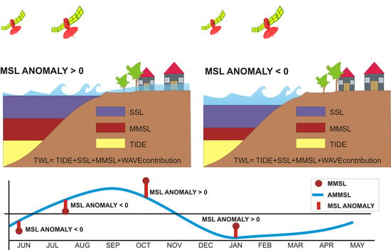
2.3.1. MMSL, AMMSL and MSL Anomalies
2.3.2. SSL
2.3.3. TIDE
2.3.4. Correlation of Seasonal MSL with Storm Impact Database
3. Results
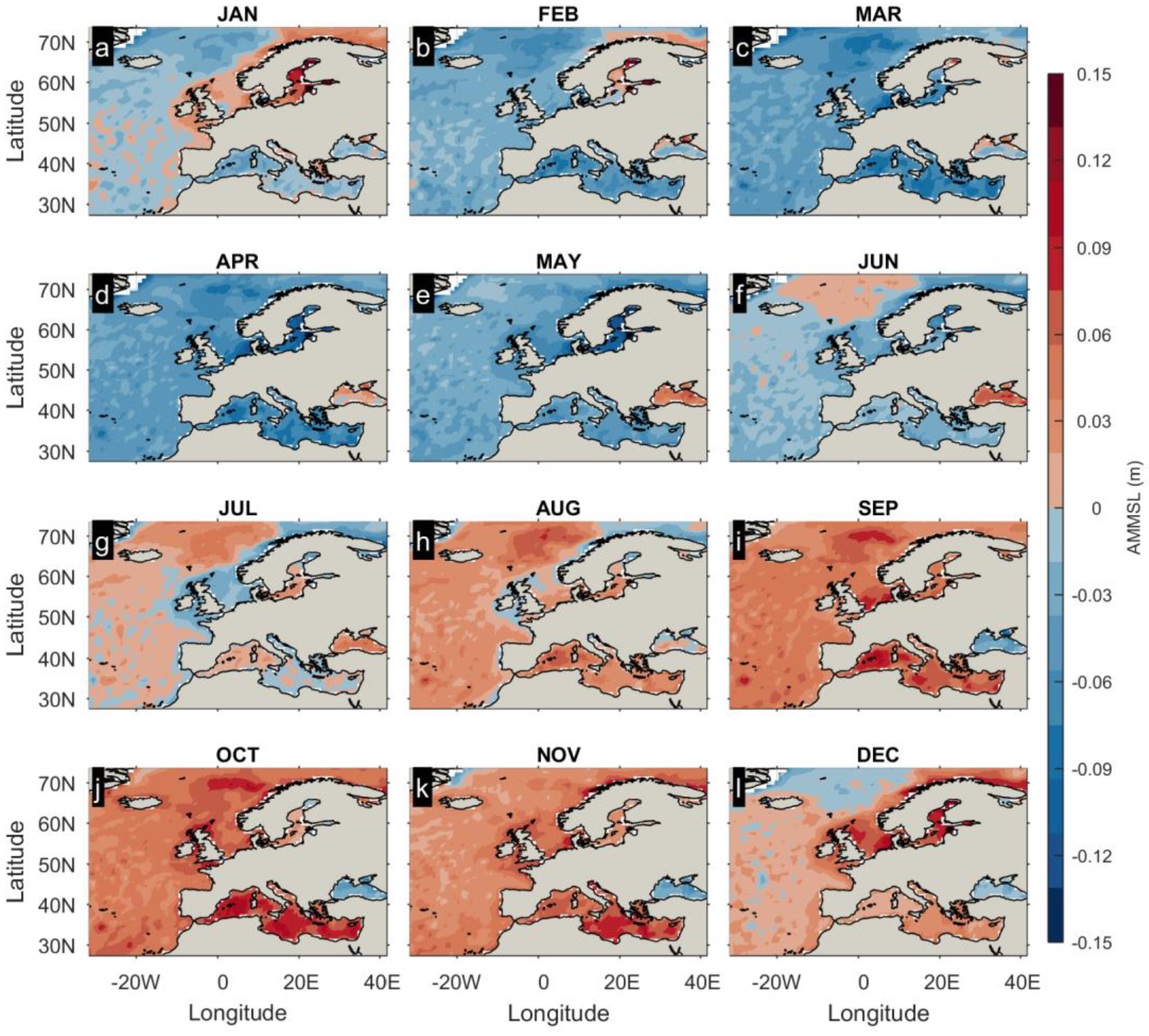
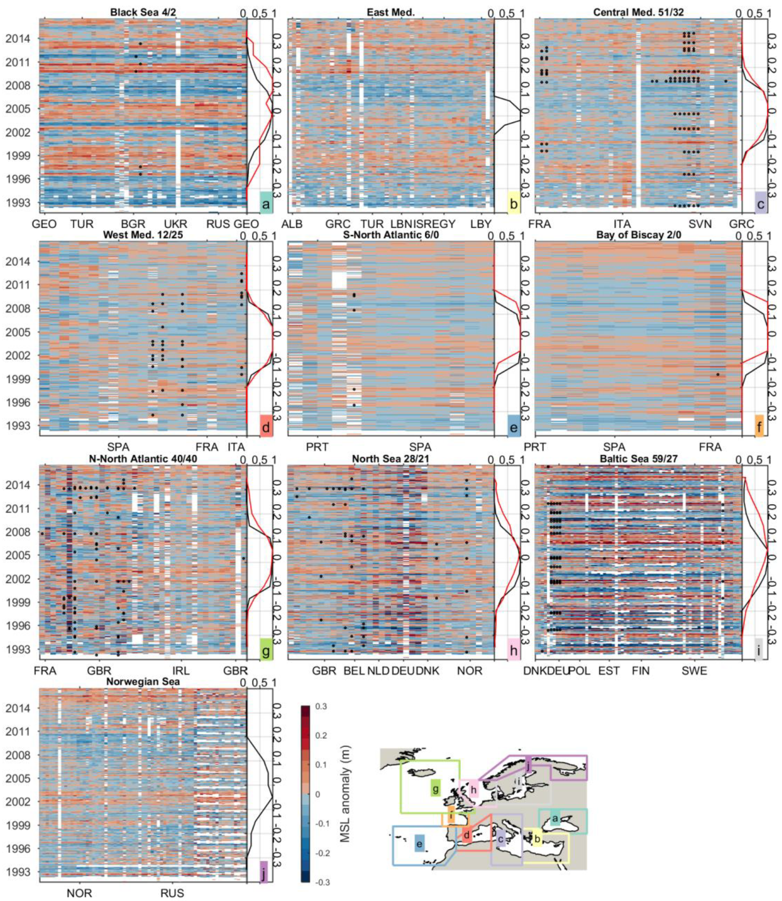
3.1. Characterization of the AMMSL and MMSL
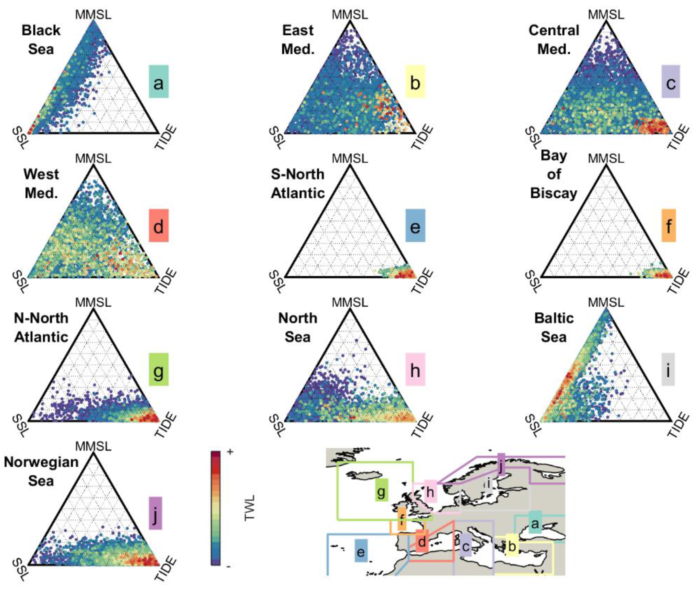
3.2. Correlation of AMMSL and MMSL with Storm Impact Database
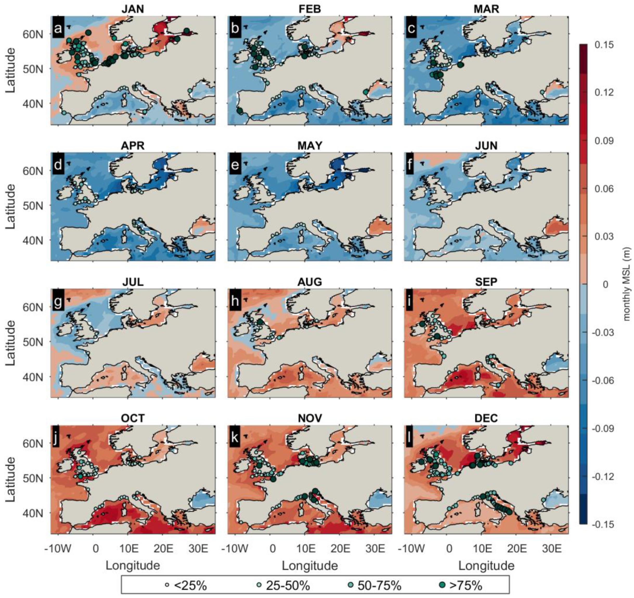
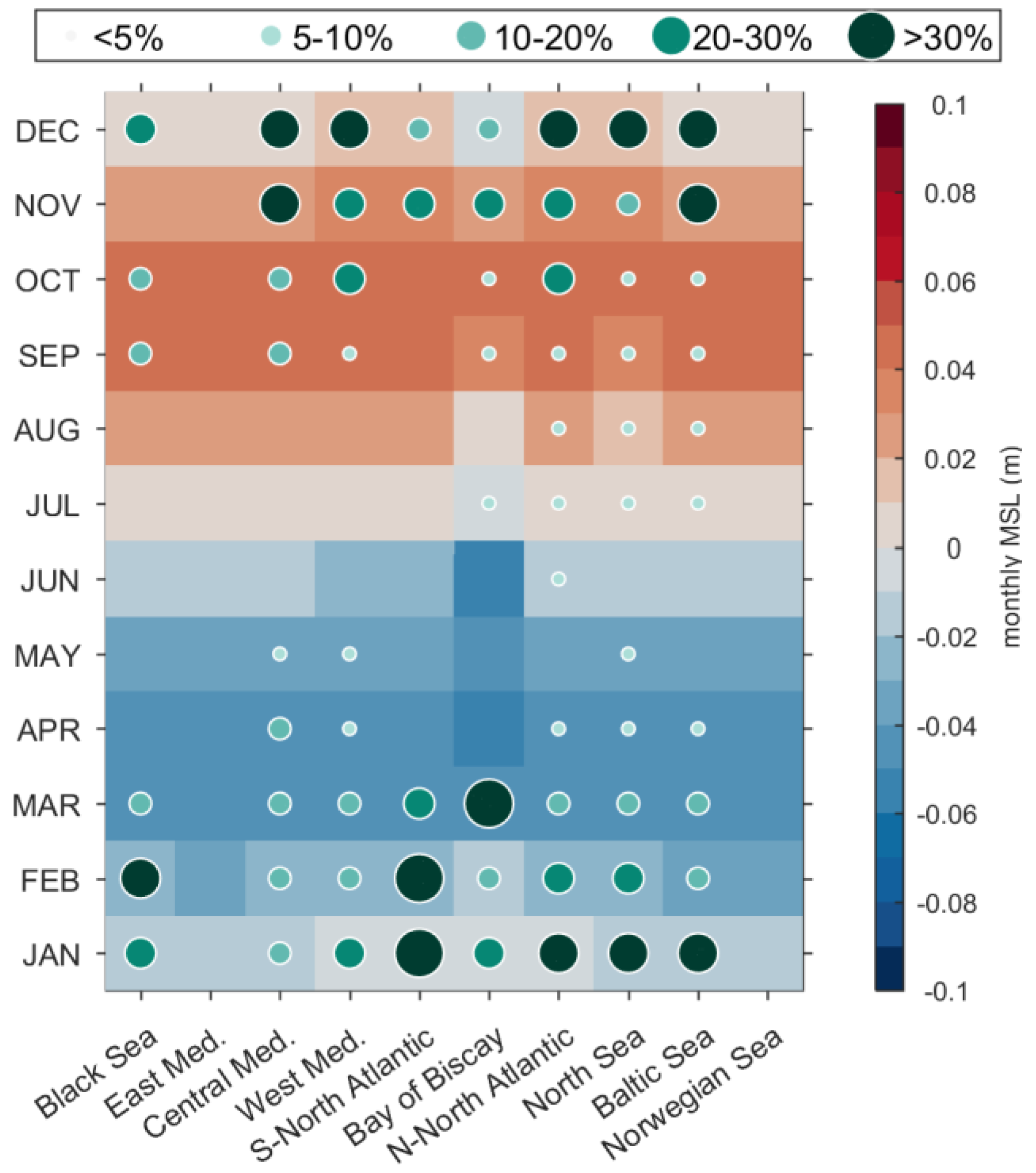
3.3. Correlation of Monthly MSL Anomalies with Storm Impact Database
4. Discussion
4.1. Time–Space Variations of Seasonal MSL and Interannual Variability
4.2. Correlation of Monthly MSL Anomalies with Storm Impact Database
4.3. Limitations and Future Research
5. Summary and Conclusions
Author Contributions
Funding
Acknowledgments
Conflicts of Interest
References
- Tessler, Z.D.; Vörösmarty, C.J.; Grossberg, M.; Gladkova, I.; Aizenman, H.; Syvitski, J.P.M.; Foufoula-Georgiou, E. Profiling risk and sustainability in coastal deltas of the world. Science 2015, 349, 638–643. [Google Scholar] [CrossRef] [PubMed] [Green Version]
- Antonellini, M.; Giambastiani, B.M.S.; Greggio, N.; Bonzi, L.; Calabrese, L.; Luciani, P.; Perini, L.; Severi, P. Processes governing natural land subsidence in the shallow coastal aquifer of the Ravenna coast, Italy. Catena 2019, 172, 76–86. [Google Scholar] [CrossRef]
- Taramelli, A.; Di Matteo, L.; Ciavola, P.; Guadagnano, F.; Tolomei, C. Temporal evolution of patterns and processes related to subsidence of the coastal area surrounding the Bevano River mouth (Northern Adriatic)—Italy. Ocean Coast. Manag. 2015, 108, 74–88. [Google Scholar] [CrossRef]
- Haigh, I.D.; Wadey, M.P.; Wahl, T.; Ozsoy, O.; Nicholls, R.J.; Brown, J.M.; Horsburgh, K.; Gouldby, B. Spatial and temporal analysis of extreme sea level and storm surge events around the coastline of the UK. Sci. Data 2016, 3, 160107. [Google Scholar] [CrossRef] [PubMed] [Green Version]
- Nicholls, R.J.; Cazenave, A. Sea-level rise and its impact on coastal zones. Science 2010, 328, 1517–1520. [Google Scholar] [CrossRef]
- Collet, I.; Engelbert, A. Archive: Coastal Regions—Population Statistics—Statistics Explained. 2013. Available online: https://ec.europa.eu/eurostat/statistics-explained/index.php/Archive:Coastal_regions_-_population_statistics (accessed on 21 February 2019).
- Haigh, I.D.; Ozsoy, O.; Wadey, M.P.; Nicholls, R.J.; Gallop, S.L.; Wahl, T.; Brown, J.M. An improved database of coastal flooding in the United Kingdom from 1915 to 2016. Sci. Data 2017, 4. [Google Scholar] [CrossRef] [Green Version]
- Paprotny, D.; Morales-Nápoles, O.; Jonkman, S.N. HANZE: A pan-European database of exposure to natural hazards and damaging historical floods since 1870. Earth Syst. Sci. Data 2018, 10, 565–581. [Google Scholar] [CrossRef] [Green Version]
- Ciavola, P.; Harley, M.D.; den Heijer, C. The RISC-KIT storm impact database: A new tool in support of DRR. Coast. Eng. 2018, 134, 24–32. [Google Scholar] [CrossRef]
- Lamb, H.; Frydendahl, K. Historic Storms of the North. Sea, British Isles and Northwest Europe; Cambridge University Press: Cambridge, UK, 1991. [Google Scholar]
- Bertin, X.; Li, K.; Roland, A.; Zhang, Y.J.; François Breilh, J.; Chaumillon, E. A modeling-based analysis of the flooding associated with Xynthia, central Bay of Biscay. Coast. Eng. 2014, 94, 80–89. [Google Scholar] [CrossRef]
- Garnier, E.; Ciavola, P.; Spencer, T.; Ferreira, O.; Armaroli, C.; McIvor, A. Historical analysis of storm events: Case studies in France, England, Portugal and Italy. Coast. Eng. 2018, 134, 10–23. [Google Scholar] [CrossRef] [Green Version]
- Paprotny, D.; Sebastian, A.; Morales-Nápoles, O.; Jonkman, S.N. Trends in flood losses in Europe over the past 150 years. Nat. Commun. 2018. [Google Scholar] [CrossRef] [PubMed]
- Wadey, M.P.; Haigh, I.D.; Nicholls, R.J.; Brown, J.M.; Horsburgh, K.; Carroll, B.; Gallop, S.L.; Mason, T.; Bradshaw, E. A comparison of the 31 January–1 February 1953 and 5–6 December 2013 coastal flood events around the UK. Front. Mar. Sci. 2015, 2. [Google Scholar] [CrossRef] [Green Version]
- Jevrejeva, S.; Jackson, L.P.; Riva, R.E.M.; Grinsted, A.; Moore, J.C. Coastal sea level rise with warming above 2 °C. Proc. Natl. Acad. Sci. USA 2016, 113, 13342–13347. [Google Scholar] [CrossRef] [PubMed] [Green Version]
- Howard, T.; Palmer, M.D.; Bricheno, L.M. Contributions to 21st century projections of extreme sea-level change around the UK. Environ. Res. Commun. 2019, 1, 095002. [Google Scholar] [CrossRef]
- Vousdoukas, M.I.; Mentaschi, L.; Voukouvalas, E.; Verlaan, M.; Feyen, L. Extreme sea levels on the rise along Europe’s coasts. Earth’s Future 2017, 5, 304–323. [Google Scholar] [CrossRef]
- Vousdoukas, M.I.; Mentaschi, L.; Voukouvalas, E.; Bianchi, A.; Dottori, F.; Feyen, L. Climatic and socioeconomic controls of future coastal flood risk in Europe. Nat. Clim. Chang. 2018, 8, 776–780. [Google Scholar] [CrossRef]
- Wankang, Y.; Baoshu, Y.; Xingru, F.; Dezhou, Y.; Guandong, G.; Haiying, C. The effect of nonlinear factors on tide-surge interaction: A case study of Typhoon Rammasun in Tieshan Bay, China. Estuar. Coast. Shelf Sci. 2019, 219, 420–428. [Google Scholar] [CrossRef]
- Horsburgh, K.J.; Wilson, C. Tide-surge interaction and its role in the distribution of surge residuals in the North Sea C8—C08003. J. Geophys. Res. Ocean. 2007, 112. [Google Scholar] [CrossRef] [Green Version]
- Dietrich, J.C.; Bunya, S.; Westerink, J.J.; Ebersole, B.A.; Smith, J.M.; Atkinson, J.H.; Jensen, R.; Resio, D.T.; Luettich, R.A.; Dawson, C.; et al. A High-Resolution Coupled Riverine Flow, Tide, Wind, Wind Wave, and Storm Surge Model for Southern Louisiana and Mississippi. Part II: Synoptic Description and Analysis of Hurricanes Katrina and Rita. Mon. Weather Rev. 2010, 138, 378–404. [Google Scholar] [CrossRef] [Green Version]
- Bertin, X.; Bruneau, N.; Breilh, J.-F.; Fortunato, A.B.; Karpytchev, M. Importance of wave age and resonance in storm surges: The case Xynthia, Bay of Biscay. Ocean. Model. 2012, 42, 16–30. [Google Scholar] [CrossRef]
- Bevacqua, E.; Maraun, D.; Vousdoukas, M.I.; Voukouvalas, E.; Vrac, M.; Mentaschi, L.; Widmann, M. Higher potential compound flood risk in Northern Europe under anthropogenic climate change. Sci. Adv. 2019, 9. [Google Scholar] [CrossRef] [PubMed] [Green Version]
- Paprotny, D.; Vousdoukas, M.I.; Morales-Nápoles, O.; Jonkman, S.N.; Feyen, L. Pan-European hydrodynamic models and their ability to identify compound floods. Nat. Hazards. 2020, 101, 933–957. [Google Scholar] [CrossRef] [Green Version]
- Vinogradov, S.V.; Ponte, R.M.; Heimbach, P.; Wunsch, C. The mean seasonal cycle in sea level estimated from a data-constrained general circulation model. J. Geophys. Res. 2008, 113, C03032. [Google Scholar] [CrossRef]
- Jordà, G.; Gomis, D. On the interpretation of the steric and mass components of sea level variability: The case of the Mediterranean basin. J. Geophys. Res. Ocean. 2013, 118, 953–963. [Google Scholar] [CrossRef] [Green Version]
- Wu, Q.; Zhang, X.; Church, J.A.; Hu, J. Variability and change of sea level and its components in the Indo-Pacific region during the altimetry era. J. Geophys. Res. Ocean. 2017, 122, 1862–1881. [Google Scholar] [CrossRef]
- Kleinherenbrink, M.; Riva, R.; Frederikse, T.; Merrifield, M.; Wada, Y. Trends and interannual variability of mass and steric sea level in the Tropical Asian Seas. J. Geophys. Res. Ocean. 2017, 122, 6254–6276. [Google Scholar] [CrossRef]
- Tsimplis, M.N.; Woodworth, P.L. The global distribution of the seasonal sea level cycle calculated from coastal tide gauge data. J. Geophys. Res. 1994, 99, 16031–16039. [Google Scholar] [CrossRef]
- Woodworth, P.L.; Melet, A.; Marcos, M.; Ray, R.D.; Wöppelmann, G.; Sasaki, Y.N.; Cirano, M.; Hibbert, A.; Huthnance, J.M.; Monserrat, S.; et al. Forcing Factors Affecting Sea Level Changes at the Coast. Surv. Geophys. 2019, 40, 1351–1397. [Google Scholar] [CrossRef] [Green Version]
- Gómez-Enri, J.; Aboitiz, A.; Tejedor, B.; Villares, P. Seasonal and interannual variability in the Gulf of Cadiz: Validation of gridded altimeter products. Estuar. Coast. Shelf Sci. 2012, 96, 114–121. [Google Scholar] [CrossRef]
- Laiz, I.; Ferrer, L.; Plomaritis, T.A.; Charria, G. Effect of river runoff on sea level from in-situ measurements and numerical models in the Bay of Biscay. Deep. Res. Part. II Top. Stud. Oceanogr. 2014, 106, 49–67. [Google Scholar] [CrossRef] [Green Version]
- Laiz, I.; Gómez-Enri, J.; Tejedor, B.; Aboitiz, A.; Villares, P. Seasonal sea level variations in the Gulf of Cadiz continental shelf from in-situ measurements and satellite altimetry. Cont. Shelf Res. 2013, 53, 77–88. [Google Scholar] [CrossRef]
- Antonov, J.I.; Levitus, S.; Boyer, T.P. Steric sea level variations during 1957-1994: Importance of salinity. J. Geophys. Res. C Ocean. 2002, 107. [Google Scholar] [CrossRef]
- Laiz, I.; Tejedor, B.; Gómez-Enri, J.; Aboitiz, A.; Villares, P. Contributions to the sea level seasonal cycle within the Gulf of Cadiz (Southwestern Iberian Peninsula). J. Mar. Syst. 2016, 159, 55–66. [Google Scholar] [CrossRef]
- Ceres, R.L.; Forest, C.E.; Keller, K. Understanding the detectability of potential changes to the 100-year peak storm surge. Clim. Chang. 2017, 145, 221–235. [Google Scholar] [CrossRef]
- Menéndez, M.; Woodworth, P.L. Changes in extreme high water levels based on a quasi-global tide-gauge data set. J. Geophys. Res. Ocean. 2010, 115, C10011. [Google Scholar] [CrossRef] [Green Version]
- Cid, A.; Castanedo, S.; Abascal, A.J.; Menéndez, M.; Medina, R. A high resolution hindcast of the meteorological sea level component for Southern Europe: The GOS dataset. Clim. Dyn. 2014, 43, 2167–2184. [Google Scholar] [CrossRef]
- Stramska, M.; Kowalewska-Kalkowska, H.; Świrgoń, M. Seasonal variability in the Baltic Sea level. Oceanologia 2013, 55, 787–807. [Google Scholar] [CrossRef]
- De Biasio, F.; Bajo, M.; Vignudelli, S.; Umgiesser, G.; Zecchetto, S. ESA DUE eSurge-Venice project. Eur. J. Remote Sens. 2017, 50, 428–441. [Google Scholar] [CrossRef] [Green Version]
- Woodworth, P.L.; Menéndez, M. Changes in the mesoscale variability and in extreme sea levels over two decades as observed by satellite altimetry. J. Geophys. Res. Ocean. 2015, 120, 64–77. [Google Scholar] [CrossRef] [Green Version]
- Cipollini, P.; Calafat, F.M.; Jevrejeva, S.; Melet, A.; Prandi, P. Monitoring Sea Level in the Coastal Zone with Satellite Altimetry and Tide Gauges. Surv. Geophys. 2017, 38, 33–57. [Google Scholar] [CrossRef] [PubMed] [Green Version]
- Andersen, O.B.; Cheng, Y.; Deng, X.; Steward, M.; Gharineiat, Z. Using satellite altimetry and tide gauges for storm surge warning. In IAHS-AISH Proceedings and Reports; Copernicus GmbH: Göttingen, Germany, 2014; Volume 365, pp. 28–34. [Google Scholar]
- Passaro, M.; Cipollini, P.; Benveniste, J. Annual sea level variability of the coastal ocean: The Baltic Sea-North Sea transition zone. J. Geophys. Res. Ocean. 2015, 120, 3061–3078. [Google Scholar] [CrossRef] [Green Version]
- Calafat, F.M.; Wahl, T.; Lindsten, F.; Williams, J.; Frajka-Williams, E. Coherent modulation of the sea-level annual cycle in the United States by Atlantic Rossby waves. Nat. Commun. 2018, 9, 1–13. [Google Scholar] [CrossRef] [Green Version]
- Dangendorf, S.; Wahl, T.; Mudersbach, C.; Jensen, J. The Seasonal Mean Sea Level Cycle in the Southeastern North Sea. J. Coast. Res. 2013, 165, 1915–1920. [Google Scholar] [CrossRef]
- Copernicus—Marine Environment Monitoring Service. Available online: https://marine.copernicus.eu/ (accessed on 1 October 2018).
- Duacs | Altimetry Data for Sea Level Studies & Applications. Available online: https://duacs.cls.fr/ (accessed on 13 January 2018).
- CMEMS. QUID forSea Level TAC DUACS Products; Available online: https://resources.marine.copernicus.eu/documents/QUID/CMEMS-SL-QUID-008-032-051.pdf (accessed on 21 February 2019).
- Carrère, L.; Lyard, F. Modeling the barotropic response of the global ocean to atmospheric wind and pressure forcing—Comparisons with observations. Geophys. Res. Lett. 2003, 30. [Google Scholar] [CrossRef] [Green Version]
- Carrere, L.; Lyard, F.; Cancet, M.; Guillot, A.; Dupuy, S.; Carrère, L.F.; Lyard, M.; Cancet, A.; Guillot, N. Picot, 2015: FES2014: A New Tidal Model Onthe Global Ocean with Enhanced Accuracy in Shallow Seas and in the Arctic Region, OSTST2015. 2014. Available online: http://meetings.aviso.altimetry.fr/fileadmin/user_upload/tx_ausyclssemi (accessed on 1 January 2019).
- Pawlowicz, R.; Beardsley, B.; Lentz, S. Classical tidal harmonic analysis including error estimates in MATLAB using T_TIDE. Comput. Geosci. 2002, 28, 929–937. [Google Scholar] [CrossRef]
- Dangendorf, S.; Arns, A.; Pinto, J.G.; Ludwig, P.; Jensen, J. The exceptional influence of storm ‘Xaver’ on design water levels in the German Bight. Environ. Res. Lett. 2016, 11, 054001. [Google Scholar] [CrossRef]
- Serafin, K.A.; Ruggiero, P.; Stockdon, H.F. The relative contribution of waves, tides, and nontidal residuals to extreme total water levels on U.S. West Coast sandy beaches. Geophys. Res. Lett. 2017, 44, 1839–1847. [Google Scholar] [CrossRef]
- Avsar, N.B.; Jin, S.; Kutoglu, H.; Gurbuz, G. Sea level change along the Black Sea coast from satellite altimetry, tide gauge and GPS observations. Geod. Geodyn. 2016, 7, 50–55. [Google Scholar] [CrossRef] [Green Version]
- Criado-Aldeanueva, F.; Del Río Vera, J.; García-Lafuente, J. Steric and mass-induced Mediterranean sea level trends from 14 years of altimetry data. Glob. Planet. Chang. 2008, 60, 563–575. [Google Scholar] [CrossRef]
- Marcos, M.; Tsimplis, M.N. Forcing of coastal sea level rise patterns in the North Atlantic and the Mediterranean Sea. Geophys. Res. Lett. 2007, 34. [Google Scholar] [CrossRef]
- Legeais, J.F.; Ablain, M.; Zawadzki, L.; Zuo, H.; Johannessen, J.A.; Scharffenberg, M.G.; Fenoglio-Marc, L.; Joana Fernandes, M.; Baltazar Andersen, O.; Rudenko, S.; et al. An improved and homogeneous altimeter sea level record from the ESA Climate Change Initiative. Earth Syst. Sci. Data 2018, 10, 281–301. [Google Scholar] [CrossRef] [Green Version]
- Ruiz Etcheverry, L.A.; Saraceno, M.; Piola, A.R.; Valladeau, G.; Möller, O.O. A comparison of the annual cycle of sea level in coastal areas from gridded satellite altimetry and tide gauges. Cont. Shelf Res. 2015, 92, 87–97. [Google Scholar] [CrossRef]
- Medvedev, I.P. Seasonal fluctuations of the Baltic Sea level. Russ. Meteorol. Hydrol. 2014, 39, 814–822. [Google Scholar] [CrossRef]
- Pajak, K.; Kowalczyk, K. A comparison of seasonal variations of sea level in the southern Baltic Sea from altimetry and tide gauge data. Adv. Sp. Res. 2019, 63, 1768–1780. [Google Scholar] [CrossRef]
- Mork, K.A.; Skagseth, Ø. Annual Sea Surface Height Variability in the Nordic Seas. In The Nordic Seas: An Integrated Perspective: Oceanography, Climatology, Biogeochemistry, and Modeling; American Geophysical Union: Washintong, DC, USA, 2005; pp. 51–64. [Google Scholar]
- Stanev, E.V.; Le Traon, P.-Y.; Peneva, E.L. Sea level variations and their dependency on meteorological and hydrological forcing: Analysis of altimeter and surface data for the Black Sea. J. Geophys. Res. Ocean. 2000, 105, 17203–17216. [Google Scholar] [CrossRef] [Green Version]
- García-García, D.; Chao, B.F.; Boy, J.P. Steric and mass-induced sea level variations in the Mediterranean Sea revisited. J. Geophys. Res. Ocean. 2010, 115, C12016. [Google Scholar] [CrossRef] [Green Version]
- Dangendorf, S.; Calafat, F.M.; Arns, A.; Wahl, T.; Haigh, I.D.; Jensen, J. Mean sea level variability in the North Sea: Processes and implications. J. Geophys. Res. Ocean. 2014, 119, 6820–6841. [Google Scholar] [CrossRef] [Green Version]
- Barbosa, S.M.; Donner, R.V. Long-term changes in the seasonality of Baltic sea level. Tellus A Dyn. Meteorol. Oceanogr. 2016, 68, 30540. [Google Scholar] [CrossRef]
- Hünicke, B.; Zorita, E. Influence of temperature and precipitation on decadal Baltic Sea level variations in the 20th century. Tellus, Ser. A Dyn. Meteorol. Oceanogr. 2006, 58, 141–153. [Google Scholar] [CrossRef] [Green Version]
- Lisitzin, E. Sea Level Changes; Elsevier Oceanography Series: Amsterdam, The Netherlands, 1974; ISBN 0444411577. [Google Scholar]
- Sterlini, P.; de Vries, H.; Katsman, C. Sea surface height variability in the North East Atlantic from satellite altimetry. Clim. Dyn. 2016, 47, 1285–1302. [Google Scholar] [CrossRef] [Green Version]
- Dangendorf, S.; Wahl, T.; Hein, H.; Jensen, J.; Mai, S.; Mudersbach, C. Mean Sea Level Variability and Influence of the North Atlantic Oscillation on Long-Term Trends in the German Bight. Water 2012, 4, 170–195. [Google Scholar] [CrossRef]
- Benveniste, J.; Cazenave, A.; Vignudelli, S.; Fenoglio-Marc, L.; Shah, R.; Almar, R.; Andersen, O.B.; Birol, F.; Bonnefond, P.; Bouffard, J.; et al. Requirements for a coastal hazards observing system. Front. Mar. Sci. 2019. [Google Scholar] [CrossRef] [Green Version]
- Passaro, M.; Rose, S.K.; Andersen, O.B.; Boergens, E.; Calafat, F.M.; Dettmering, D.; Benveniste, J. ALES+: Adapting a homogenous ocean retracker for satellite altimetry to sea ice leads, coastal and inland waters. Remote Sens. Environ. 2018, 211, 456–471. [Google Scholar] [CrossRef] [Green Version]
- Birol, F.; Fuller, N.; Lyard, F.; Cancet, M.; Niño, F.; Delebecque, C.; Fleury, S.; Toublanc, F.; Melet, A.; Saraceno, M.; et al. Coastal applications from nadir altimetry: Example of the X-TRACK regional products. Adv. Sp. Res. 2017, 59, 936–953. [Google Scholar] [CrossRef]
- Marcos, M.; Rohmer, J.; Vousdoukas, M.I.; Mentaschi, L.; Le Cozannet, G.; Amores, A. Increased Extreme Coastal Water Levels Due to the Combined Action of Storm Surges and Wind Waves. Geophys. Res. Lett. 2019, 46, 4356–4364. [Google Scholar] [CrossRef] [Green Version]
- Melet, A.; Meyssignac, B.; Almar, R.; Le Cozannet, G. Under-estimated wave contribution to coastal sea-level rise. Nat. Clim. Chang. 2018, 8, 234–239. [Google Scholar] [CrossRef]
- Serafin, K.A.; Ruggiero, P. Simulating extreme total water levels using a time-dependent, extreme value approach. J. Geophys. Res. C Ocean. 2014, 119, 6305–6329. [Google Scholar] [CrossRef] [Green Version]
- Harley, M.D.; Valentini, A.; Armaroli, C.; Perini, L.; Calabrese, L.; Ciavola, P. Can an early-warning system help minimize the impacts of coastal storms? A case study of the 2012 Halloween storm, northern Italy. Nat. Hazards Earth Syst. Sci. 2016, 16, 209–222. [Google Scholar] [CrossRef] [Green Version]
- RiscKit Storm Database. Available online: http://risckit.cloudapp.net/risckit/#/ (accessed on 16 November 2019).
- Wolski, T.; Wiśniewski, B.; Giza, A.; Kowalewska-Kalkowska, H.; Boman, H.; Grabbi-Kaiv, S.; Hammarklint, T.; Holfort, J.; Lydeikaite, Z. Extreme sea levels at selected stations on the Baltic Sea coast. Oceanologia 2014, 2, 259–290. [Google Scholar] [CrossRef] [Green Version]
- Fernández-Montblanc, T.; Vousdoukas, M.I.; Ciavola, P.; Voukouvalas, E.; Mentaschi, L.; Breyiannis, G.; Feyen, L.; Salamon, P. Towards robust pan-European storm surge forecasting. Ocean Model. 2019, 133, 129–144. [Google Scholar] [CrossRef]
- Muis, S.; Verlaan, M.; Winsemius, H.C.; Aerts, J.C.J.H.; Ward, P.J. A global reanalysis of storm surges and extreme sea levels. Nat. Commun. 2016, 7, 11969. [Google Scholar] [CrossRef] [PubMed] [Green Version]
- Vousdoukas, M.I.; Mentaschi, L.; Voukouvalas, E.; Verlaan, M.; Jevrejeva, S.; Jackson, L.P.; Feyen, L. Global probabilistic projections of extreme sea levels show intensification of coastal flood hazard. Nat. Commun. 2018, 9, 2360. [Google Scholar] [CrossRef] [PubMed] [Green Version]


| Region | Black Sea | Central Med. | West Med. | S-North Atlantic | Bay of Biscay | N-North Atlantic | NorthSea | BalticSea |
|---|---|---|---|---|---|---|---|---|
| SSL | −0.06 (0.86) | 0.03 (0.94) | 0.18 (0.57) | 0.52 (0.08) | 0.37 (0.24) | 0.97 (3 × 10⁻⁷) | 0.90 (6 × 10⁻⁵) | −0.79 (2 × 10⁻³) |
| TIDE | 0.14 (0.66) | −0.73 (7 × 10⁻³) | −0.78 (3 × 10⁻³) | −0.16 (0.63) | −0.32 (0.32) | −0.94 (4 × 10⁻⁶) | −0.88 (2 × 10⁻⁴) | −0.54 (0.07) |
| MMSL | 0.05 (0.87) | 0.73 (7 × 10⁻³) | 0.29 (0.36) | −0.21 (0.52) | 0.12 (0.70) | 0.45 (0.14) | 0.67 (0.02) | 0.77 (4 × 10⁻³) |
| Region | Black Sea | East Med. | Central Med. | West Med. | S-North Atlantic | Bay of Biscay | N-North Atlantic | North Sea | Baltic Sea | Norwegian Sea |
|---|---|---|---|---|---|---|---|---|---|---|
| Corr. coefficient | −0.1 | - | 0.28 | 0.32 | −0.22 | −0.14 | 0.30 | 0.02 | 0.10 | - |
| p-value | 0.75 | - | 0.38 | 0.31 | 0.49 | 0.67 | 0.35 | 0.95 | 0.76 | - |
| Region | Black Sea | Central Med. | West Med. | S-North Atlantic | Bay of Biscay | N-North Atlantic | North Sea | Baltic Sea |
|---|---|---|---|---|---|---|---|---|
| t-test (0.05) | 0 (0.28) | 1 (3 × 10⁻⁴) | 0 (0. 86) | 1 (3 × 10⁻³) | 0 (0.08) | 0 (0.07) | 1 (4 × 10⁻²) | 1 (3 × 10⁻⁷) |
| Mean MSL anomaly | 0.03 | 0.02 | −0.01 | 0.04 | 0.04 | 0.02 | 0.03 | 0.07 |
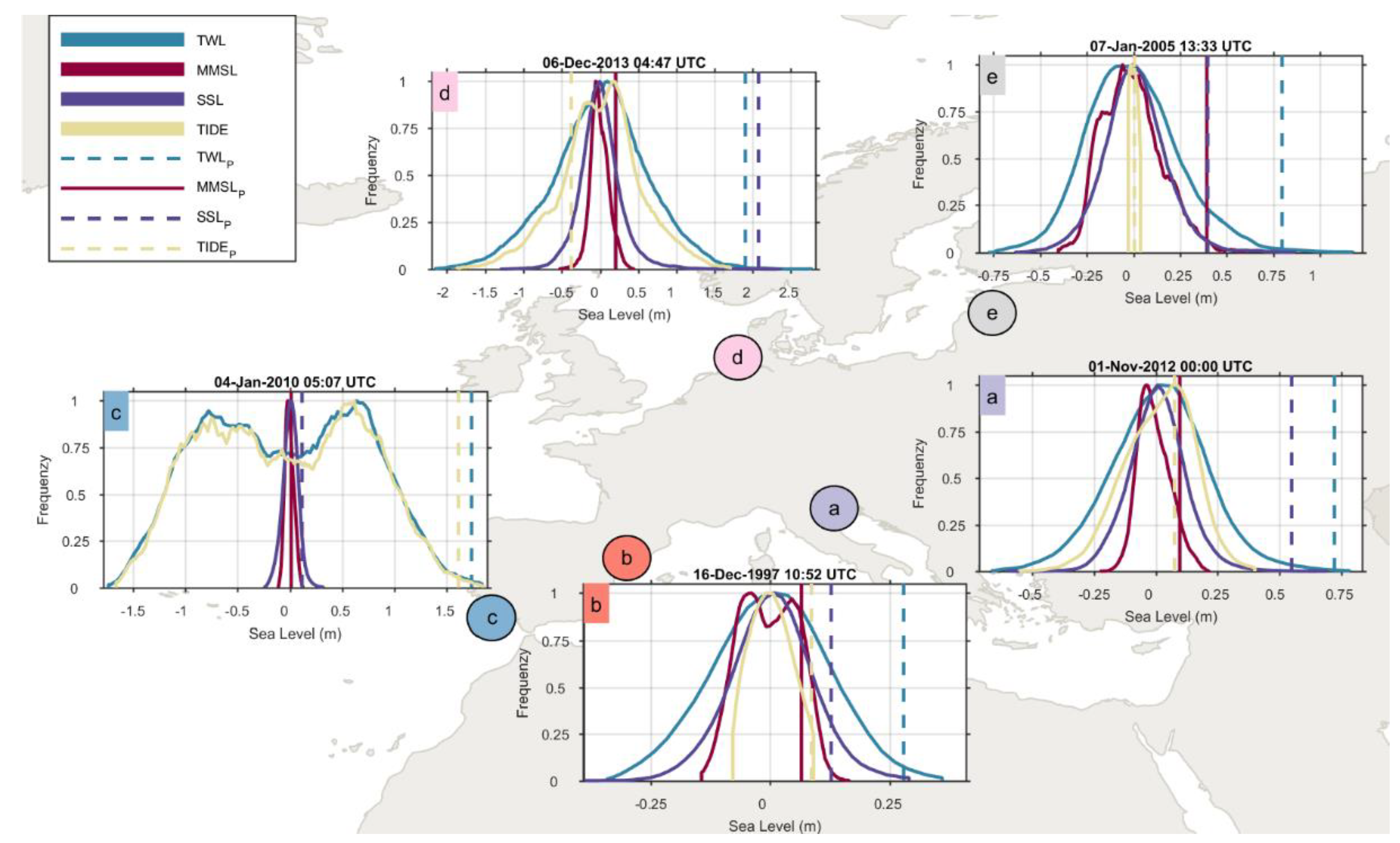
| Central Med. [77]) | West Med. [78] | S-North Atlantic [78] | North Sea ([53]) | Baltic Sea ([79]) | |
|---|---|---|---|---|---|
| TWLp. | 0.72 m (1.16 m) | 0.28 m (0.46 m) | 1.74 m (1.6 m) | 1.9 m (~4.67 m) | 0.8 m (2.22 m) |
| SSLp. | 0.55 m (0.81 m) | 0.13 m | 0.12 m | 2.08 m (2.67 m) | 0.4 m |
| TIDEp | 0.08 m (0.23 m) | 0.09 m | 1.61 m | −0.38 m (~1.5 m) | 0.01 m |
| MMSLp | 0.1 m (~0.12 m) | 0.07 m | 0.01 m | 0.21 m (0.50 m) | 0.39 |
| DATEp | 01.11.2012 00:00 (31-10-2012 23:30) | 16.12.1997 10:52 | 04.01.2010 05:07 | 06.12.2013 04:47 (06.12.2013 02:00) | 07.01.2019 13:33 (09.01.2009 06:00) |
Publisher’s Note: MDPI stays neutral with regard to jurisdictional claims in published maps and institutional affiliations. |
© 2020 by the authors. Licensee MDPI, Basel, Switzerland. This article is an open access article distributed under the terms and conditions of the Creative Commons Attribution (CC BY) license (http://creativecommons.org/licenses/by/4.0/).
Share and Cite
Fernández-Montblanc, T.; Gómez-Enri, J.; Ciavola, P. The Role of Mean Sea Level Annual Cycle on Extreme Water Levels Along European Coastline. Remote Sens. 2020, 12, 3419. https://doi.org/10.3390/rs12203419
Fernández-Montblanc T, Gómez-Enri J, Ciavola P. The Role of Mean Sea Level Annual Cycle on Extreme Water Levels Along European Coastline. Remote Sensing. 2020; 12(20):3419. https://doi.org/10.3390/rs12203419
Chicago/Turabian StyleFernández-Montblanc, Tomás, Jesús Gómez-Enri, and Paolo Ciavola. 2020. "The Role of Mean Sea Level Annual Cycle on Extreme Water Levels Along European Coastline" Remote Sensing 12, no. 20: 3419. https://doi.org/10.3390/rs12203419