Article

Evaluation of the MODIS LAI/FPAR Algorithm Based on 3D-RTM Simulations: A Case Study of Grassland

1
School of Land Science and Techniques, China University of Geosciences, Beijing 100083, China
2
Department of Earth and Environment, Boston University, Boston, MA 02215, USA
3
Department of Systems Design Engineering, University of Waterloo, Waterloo, ON N2L 3G1, Canada
*
Author to whom correspondence should be addressed.
Remote Sens. 2020, 12(20), 3391; https://doi.org/10.3390/rs12203391
Submission received: 12 August 2020 / Revised: 4 October 2020 / Accepted: 14 October 2020 / Published: 16 October 2020
(This article belongs to the Special Issue Remote Sensing of Biophysical Parameters)

Abstract

:
Uncertainty assessment of the moderate resolution imaging spectroradiometer (MODIS) leaf area index (LAI) and the fraction of photosynthetically active radiation absorbed by vegetation (FPAR) retrieval algorithm can provide a scientific basis for the usage and improvement of this widely-used product. Previous evaluations generally depended on the intercomparison with other datasets as well as direct validation using ground measurements, which mix the uncertainties from the model, inputs, and assessment method. In this study, we adopted the evaluation method based on three-dimensional radiative transfer model (3D RTM) simulations, which helps to separate model uncertainty and other factors. We used the well-validated 3D RTM LESS (large-scale remote sensing data and image simulation framework) for a grassland scene simulation and calculated bidirectional reflectance factors (BRFs) as inputs for the LAI/FPAR retrieval. The dependency between LAI/FPAR truth and model estimation serves as the algorithm uncertainty indicator. This paper analyzed the LAI/FPAR uncertainty caused by inherent model uncertainty, input uncertainty (BRF and biome classification), clumping effect, and scale dependency. We found that the uncertainties of different algorithm paths vary greatly (−6.61% and +84.85% bias for main and backup algorithm, respectively) and the “hotspot” geometry results in greatest retrieval uncertainty. For the input uncertainty, the BRF of the near-infrared (NIR) band has greater impacts than that of the red band, and the biome misclassification also leads to nonnegligible LAI/FPAR bias. Moreover, the clumping effect leads to a significant LAI underestimation (−0.846 and −0.525 LAI difference for two clumping types), but the scale dependency (pixel size ranges from 100 m to 1000 m) has little impact on LAI/FPAR uncertainty. Overall, this study provides a new perspective on the evaluation of LAI/FPAR retrieval algorithms.

Graphical Abstract

1. Introduction

Leaf area index (LAI), defined as half of the total green leaf area of per unit horizontal ground area, is a basic parameter for measuring the vegetation canopies [1,2]. This variable plays a key roles in hydrology, biogeochemistry, and ecosystem models that connect vegetation to the climate observing system through the carbon, water cycles, and radiation [3]. Fraction of photosynthetically active radiation (0.4–0.7 μm) absorbed by vegetation (FPAR) measures the proportion of the solar radiation entering at the top of the plant canopy that contributes to the photosynthetic activity [3,4,5,6]. LAI/FPAR retrieved from remote sensing observations in the reflective solar domain, are used as input parameters for models monitoring the Earth’s surface continuously and are key parameters recognized by the global climate observing system (GCOS) to describe climatic characteristics [3,7]. LAI/FPAR products, derived from atmospherically corrected surface reflectances, have entered a new era since the moderate resolution imaging spectroradiometer (MODIS) became operational in 1999 [8,9,10]. The MODIS LAI/FPAR products (MOD15), based on the radiative transfer (RT) model [11], have been widely used to corroborate global climate change [12], to serve as key inputs for terrestrial carbon cycle models [13], and to support the research of both phenomena and possible reasons of large scale vegetation dynamics [14,15,16]. Moreover, the generation of MODIS LAI/FPAR products does not depend on other LAI/FPAR datasets and they are commonly used as input and reference data for the generation and intercomparison of other products [17,18].
Intensive evaluation and validation efforts have been carried out to examine the uncertainty of MODIS LAI/FPAR products and the corresponding retrieval algorithm. These works mainly included: (1) theoretical derivation based on model mechanisms and error propagation [19]; (2) intercomparison with other LAI/FPAR products or related variables (e.g., GLASS, CYCLOPES, VIIRS) [20,21,22,23,24,25]; (3) direct validation using ground LAI/FPAR measurements [25,26]. The theoretical derivation has an explicit mathematical basis and does not require other datasets; however, this approach is highly correlated with the algorithm itself and is easily affected by model limitations and uncertainties [27,28]. Intercomparison with other LAI/FPAR products is an approach that can effectively analyze the spatio-temporal consistency of long-term LAI/FPAR, but the results cannot meet the requirement of product usage and algorithm refinement. Ground-based validations are essential as the basis of all validations, but the accuracy of this validation method includes the uncertainty of the ground measurements, the spatial heterogeneity-caused uncertainty [29] in the upscaling process from the point measurement to the pixel scale, and the product uncertainty. Above all, the previous studies mainly focused on the evaluation of product uncertainty, which introduces the coupled uncertainties from the model, inputs, and assessment method. Therefore, it would hinder the process of evaluating the uncertainty of the algorithm itself and understanding the deficiencies of the algorithm, thus hampering future improvements to the algorithm.
In the above context, real scene computer simulations provide a new approach for remote sensing evaluation and validation [30]. As computing power improves, several 3D RT models have been developed for scene simulation [31,32], such as DART (discrete anisotropic radiative transfer) [33], RAPID (radiosity applicable to porous individual objects) [34], and LESS (large-scale remote sensing data and image simulation framework) [35]. These models have become an important tool in the field of quantitative remote sensing, particularly for studying the radiometric properties of the Earth’s surface [31,36]. 3D RT models can analyze the detailed interactions between solar radiation and vegetation canopies [37], analyze the radiative properties of specific biome types [38], and help the science team define the characteristics of optical sensors through model simulation [39]. Data from simulations based on 3D RT models are widely used for model validation and evaluation. The DART model has been used in studies on the surface energy budget [40], the impact of canopy structure on satellite image texture [41], the 3D distribution of photosynthesis and primary production rates of vegetation canopies [42], and forest biophysical parameter retrieval [43,44]. The LESS model can synergistically use spectral and angular information to simulate the radiation properties of complex realistic landscapes, which can be used for simulating datasets of 3D landscapes [45]. The outputs of LESS can serve as benchmarks for retrieval algorithm evaluation since it has a solid theoretical foundation and its accuracy has already been well-assessed by comparison with other models of radiation transfer model intercomparison (RAMI) [35] and field measurements [46].
This study aimed to provide a new perspective on the evaluation of MODIS LAI/FPAR retrieval algorithms, which differs from previous research by evaluating the algorithm itself rather than the product. In this paper, a computer simulation of a real grassland scene is performed using the ray-tracing LESS model to analyze the uncertainty of the MODIS LAI/FPAR retrieval algorithm. The advantage of simulation-based model evaluation is that the uncertainty caused by a single variable can be analyzed to avoid the effects caused by the mixing of multiple factors. The uncertainty of the MODIS LAI/FPAR algorithm was evaluated by separating the model and input uncertainties. In addition, further analysis was conducted to understand the impact of scale dependency and clumping. The results can serve as guidance for improving this algorithm continuously.
The structure of this paper is organized as follows. Section 2 briefly describes the MODIS LAI/FPAR retrieval algorithm, how we use LESS to analyze the retrieval algorithm for uncertainty, and the methodologies for uncertainty evaluation. Section 3 details the results of LAI/FPAR uncertainty caused by inherent model, reflectance, and biome type uncertainties as well as the clumping effect, and scale dependency. The discussions, including the analysis of the experiment results, are detailed in Section 4. Finally, Section 5 provides some concluding remarks.

2. Materials and Methods

2.1. MODIS LAI/FPAR Retrieval Algorithm

The MODIS LAI/FPAR retrieval algorithm consists of a main algorithm based on the radiative transfer equation (RTE) and a backup algorithm using the relationship between vegetation index and LAI/FPAR. The retrieval algorithm exploits the spectral information content of MODIS surface reflectances at up to 7 spectral bands (band 1: 620–670 nm; band 2: 841–876 nm; band 3: 459–479 nm; band 4: 545–565 nm; band 5: 1230–1250 nm; band 6: 1628–1652 nm; band 7: 2105–2155 nm) [4,8]. Inputs of this algorithm include BRFs at red and near-infrared (NIR) bands (band 1 and 2), their uncertainties, sun–sensor geometry (SZA: solar zenith angle, SAA: solar azimuth angle, VZA: view zenith angle, VAA: view azimuth angle), and a biome classification map. Note that in the current algorithm version, different biome types use different RT models. Herbaceous biomes (B1: grasses and cereal crops; B2: shrubs; B3: broadleaf crops;) were modelled using 1D RT due to the good continuity of the grass distribution and in consideration of the computational efficiency. Savannas (B4) were modelled by a stationary Poisson germ-grain stochastic process (so called stochastic radiative transfer (SRT) model) [47,48]. Forest biomes (B5: evergreen broadleaf forests; B6: deciduous broadleaf forests; B7: evergreen needleleaf forests; and B8: deciduous needleleaf forests) were based on a 3D RTM (3D structures were represented by columns uniformly (deterministically) spaced on the ground). With these RTMs, the science team constructed an LAI/FPAR main algorithm based on angular information, biome type, and spectral information in which the mean and standard deviation values of the LAI and FPAR selected in the spectral retrieval space are reported for retrieval value and its uncertainty. The main look up table (LUT)-based algorithm was designed as follows. Firstly, the main algorithm evaluates a weight coefficient as a function of sun–sensor geometry, wavelength, and LAI by using a field-tested canopy reflectance model. Then it calculates the BRFs by using the weight coefficient and the same model [4,8]. The algorithm tests the eligibility of a canopy radiation model to generate the LUT file where a subset of coefficients is satisfied within a given accuracy [9]. The given atmosphere-corrected BRFs are then compared with the modeled BRFs, which are stored in the biome-specific LUT files. Finally, all candidates of LAI/FPAR are used to calculate the mean values and uncertainty of the retrieval [9]. In the case of highly dense canopies, reflectance will be saturated and insensitive to changes in canopy properties. Therefore, LAI and FPAR values acquired under saturated conditions are less reliable than those generated by unsaturated BRFs. When the main algorithm fails to localize a solution, the backup algorithm is used to retrieve values through an empirical relationship between the normalized difference vegetation index (NDVI) and the canopy LAI/FPAR [11,21]. Such retrievals are flagged in the algorithm path quality assessment (QA) variable [8], which consists of two values for the main algorithm and two values for the backup algorithm (from high quality to low): the main algorithm without saturation (QA = 0), the main algorithm with saturation (QA = 1), the backup algorithm due to sun–sensor geometry (QA = 3), and the backup algorithm due to other reasons (QA = 4) [9,14,49].

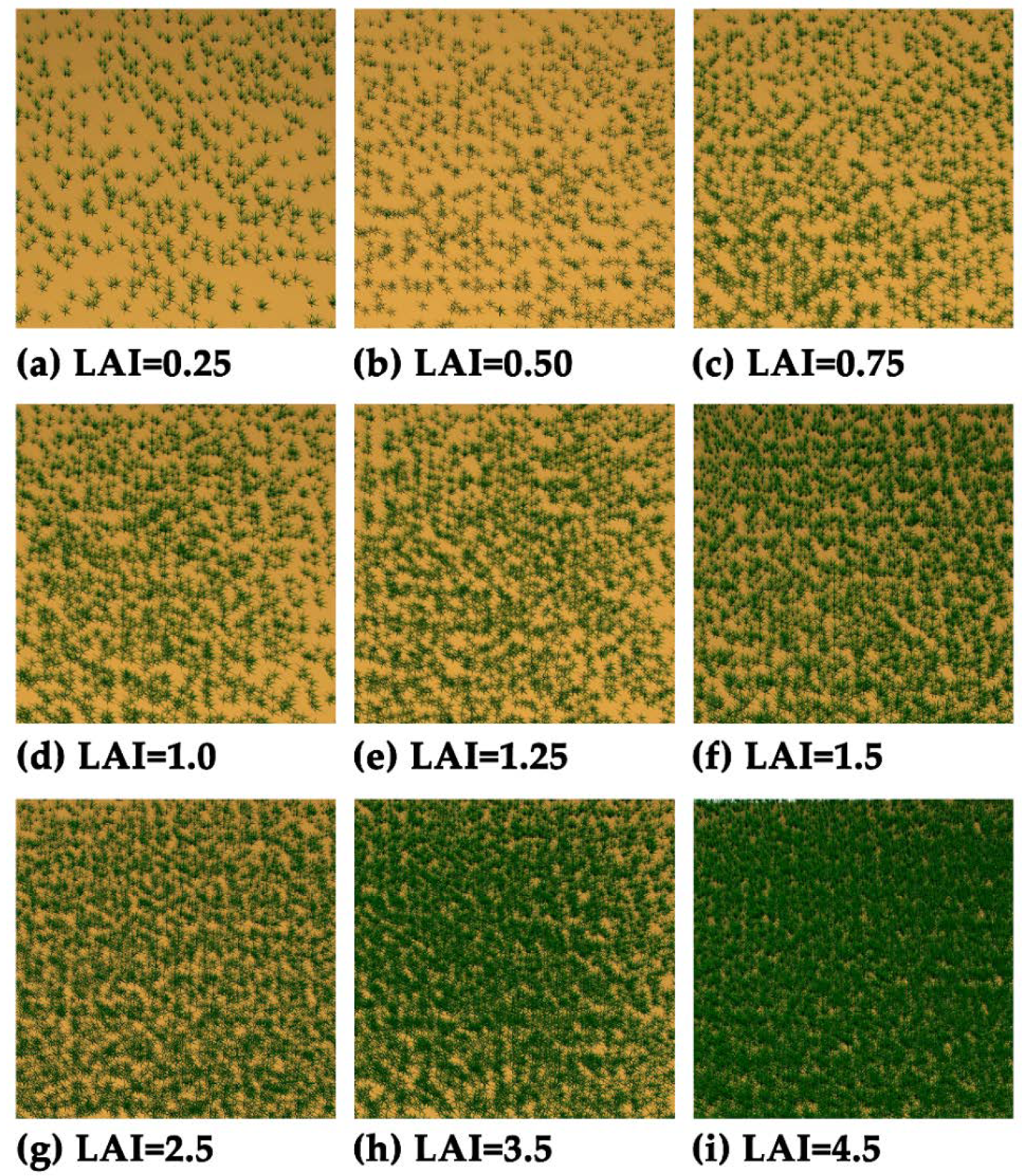
2.2. Three-Dimensional Grassland Scene Simulation

We used the newly proposed but well validated 3D RT model LESS to simulate the interaction between the solar radiation and landscape elements based on the spectral response functions (SRFs) (from ENVI software) of MODIS and calculated the scene BRFs [35,45]. LESS simulates BRFs by a weighted forward photon tracing method as well as simulated energy transfer and generates images by a backward path tracing method [35]. Qi et al. [35] described the comparison between BRFs simulated by LESS and average BRF results from other models (e.g., SPRINT3, RAYTRAN, and RAYSPREAD) over several different homogeneous and heterogeneous canopies from the RAMI website to evaluate the accuracy of LESS.
The input parameters of LESS include 3D landscape elements, optical properties, and sun–sensor geometries. The simulated scenes are covered by grass (Johnson grass) and its component spectra were obtained from the LOPEX93 dataset on the OPTICLEAF website [50]. The soil (grayish brown loam) spectra were selected from the soil spectral library in ENVI software, and the transmittance of the soil is 0 (Figure 1). Then we calculated the two MODIS bands (red: band 1 and NIR: band 2) reflectance and transmittance (see Table 1) using SRFs (the shaded part of Figure 1) of the MODIS sensor by the following equation [51]:
{ R = λ   =   λ m i n λ m a x     S λ R λ /   λ   =   λ m i n λ m a x     S λ T = λ   =   λ m i n λ m a x     S λ T λ / λ   =   λ m i n λ m a x     S λ
where, R and T are MODIS band reflectance and transmittance, respectively. The R λ and T λ are mean narrow-band reflectance and transmittance derived from the spectral curves. The S λ is the SRF value of the MODIS sensor. λ is the value of wavelength, which has a specific upper ( λ m a x : red = 670 μ m , NIR = 876 μ m ) and lower ( λ m i n : red = 620 μ m , NIR = 841 μ m ) limit for each band.
The 3D landscape elements were created with the third-party software OnyxTree, which uses the calculated reflectance and transmittance (Table 1) to make a grass 3D model (obj format file). As shown in Figure 2, we created nine randomly distributed grasslands with different LAIs (0.25, 0.50, 0.75, 1.0, 1.25, 1.5, 2.5, 3.5, and 4.5) using the LESS and grass 3D model. Moreover, LESS calculates FPAR by performing a band integration of the PAR between 380 nm and 710 nm and dividing by the incident radiation (slightly different from MODIS for which the wavelength interval is 400–800 nm) based on the LESS simulation of the collision of photons and the transfer of energy. In addition, to match the canopy structure of grasses in the MODIS LAI/FPAR retrieval algorithm (all organs other than leaves are ignored), only foliage is present in the scene. There is also only direct radiation in these scenes. The size of these scenes is 500 m × 500 m, which matches the spatial resolution of the MODIS LAI/FPAR products.

2.3. Experimental Design

We utilized the standard deviation of all LAI/FPAR candidates (StdLAI and StdFPAR), the retrieval index (RI), and the relative and absolute LAI/FPAR differences as the indicators of LAI/FPAR uncertainty. According to the uncertainty theory, StdLAI and StdFPAR are the standard deviations of all acceptable LAI/FPAR solutions in the LUT, which are the function of both the input uncertainty (biome type and BRF uncertainty) and model uncertainty [4,8]. StdLAI and StdFPAR have been proven and evaluated as quality metrics for MODIS LAI/FPAR products [28,52]. However, these two metrics have limitations due to the regularization introduced by the LUT algorithm and are artificially lowered at large LAIs [8]. Therefore, in this paper, we have also selected the RI (see Equation (2)) as an uncertainty metric, which is defined as the percentage of pixels for which the main RTE-based algorithm generates retrieval results. We note that the RI is used to characterize the overall uncertainty of all pixels [21,25,53], while StdLAI and StdFPAR are used to characterize individual pixel uncertainty.
RI   =   N u m b e r   o f   p i x e l s   r e t r i e v e d   b y   t h e   m a i n   a l g o r i t h m   T o t a l   n u m b e r   o f   p r o c e s s e d   p i x e l s  
To evaluate the consistency between true LAI/FPAR and MODIS retrievals, the difference between the simulation results of LAI (input to the LESS)/FPAR (output from the LESS) and the LAI/FPAR retrieved by the MODIS retrieval algorithm were used. The relative difference (RD, see Equation (3)) and absolute difference (AD, see Equation (4)), were utilized to quantify any differences.
RD   =   ( Retrieval Truth ) / Truth
AD   =   Retrieval Truth
Based on the uncertainty theory, the retrieval uncertainty is a function of both model and input uncertainty and is embedded in the MODIS algorithm. In this study, we explored the relationship between retrieval uncertainty and the retrieval space, sun–sensor geometry, surface reflectance uncertainty, and biome type uncertainty using the variable-controlling approach (see Table 2). We analyzed the inherent model uncertainty in two steps: 1) analysis of the retrieval space; 2) uncertainty changed with sun–sensor geometry. We obtained 4000 red-NIR BRF pairs by adding normally distributed errors (errors with 5% and 15% standard deviation) to the LESS simulated red and NIR band BRFs (1000: red without uncertainties and NIR with 5% standard deviation, 1000: red without uncertainties and NIR with 15% standard deviation, 1000: NIR without uncertainties and red with 5% standard deviation, and 1000: NIR without uncertainties and red with 15% standard deviation). Then we analyzed the LAI/FPAR uncertainty caused by BRF uncertainty within the 4 groups of samples. In addition, we analyzed uncertainties due to biome type misclassification, which is one of the main factors affecting the LAI/FPAR retrieval accuracy [4,54]. Each red-NIR BRF pair was sequentially combined with each biome type as the inputs for the MODIS LAI/FPAR algorithm. In this experiment, only B1 (grasses and cereal crops) was correct while the remaining seven combinations represented the biome type misclassification cases. Finally, we analyzed the influence of scale dependency and clumping effect (“tree groups”) [55] on the uncertainty of LAI/FPAR retrievals. We simulated a randomly distributed 1 km × 1 km scene (Figure 9a-1) and two clumping 1 km × 1 km scenes. Clumping type 1 (CT1, Figure 9a-2) had random clumping and Clumping type 2 (CT2, Figure 9a-3) was half bare ground and half grass. The LAI of the three scenes remained constant and these scenes were downscaled into four 500 m × 500 m scenes, sixteen 250 m × 250 m scenes, and one hundred 100 m × 100 m scenes for the discussion of scale dependency and clumping effect.

3. Results

3.1. Inherent Model Uncertainty

To evaluate the inherent model uncertainty of the MODIS LAI/FPAR retrieval algorithm, we analyzed the effect of the retrieval space and sun–sensor uncertainty, separately. In performing the evaluation of the retrieval space, we paid more attention to the changes in the uncertainty of algorithm paths. While the difference between the LAI/FPAR retrieval and LESS simulations were analyzed when evaluating of the sun–sensor geometry.

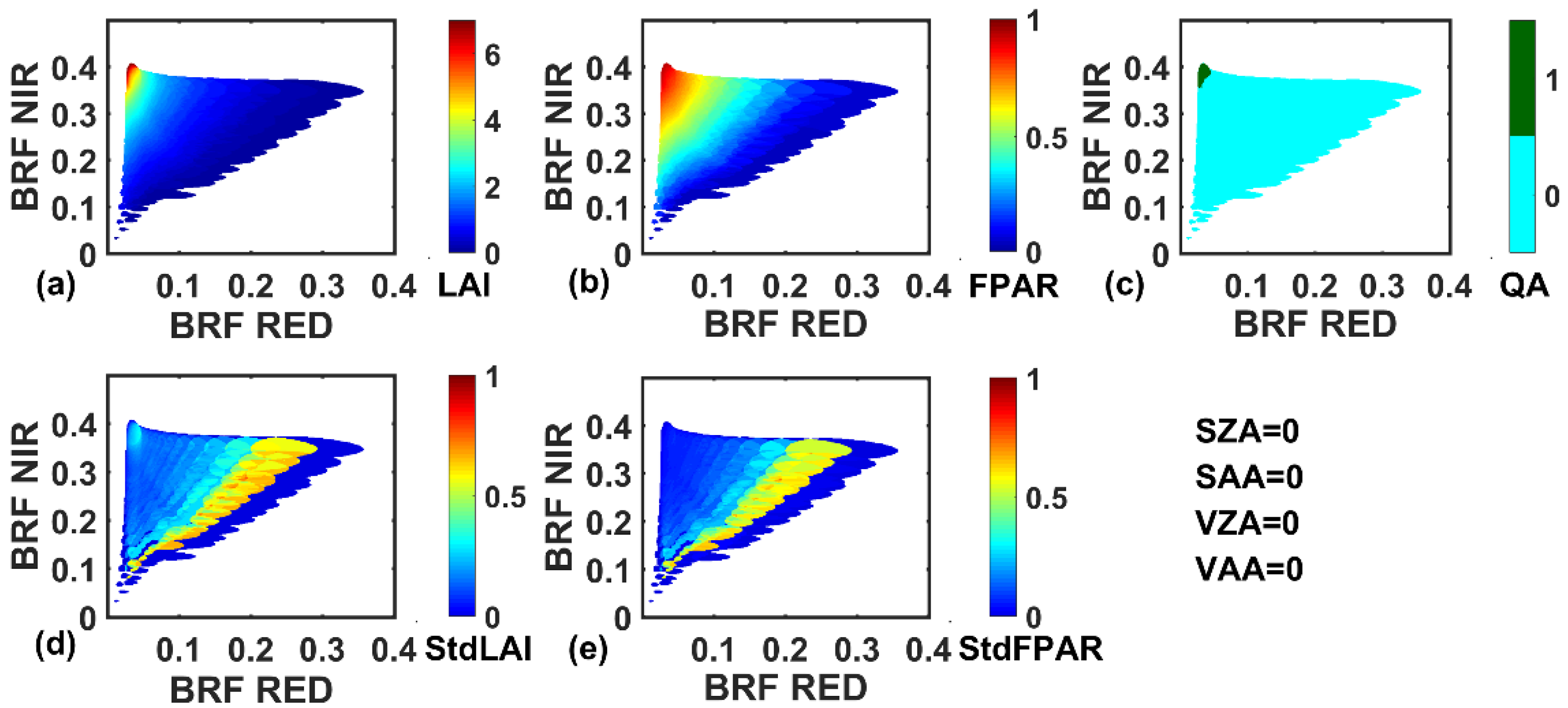
3.1.1. Analysis of Retrieval Space

Figure 3 indicates the variation of LAI/FPAR and its uncertainty in the retrieval space. As we can see, LAI/FPAR is nonlinearly related to surface reflectance (Figure 3a,b), and FPAR is also nonlinearly related to LAI. Moreover, the relationship between LAI/FPAR and its uncertainty (StdLAI and StdFPAR) is also nonlinear. The StdLAI and StdFPAR are very low for lower LAI/FPAR and then increase to the highest values, and then steadily decrease (from the bottom right to the top left of Figure 3d,e) as the LAI/FPAR gets progressively larger (from the bottom right to the top left of Figure 3a,b). It is also obvious that there is a clear division between the saturated (QA = 1) and unsaturated (QA = 0) parts where the LAI/FPAR values are higher in the saturated part (Figure 3c). Compared to the unsaturated part, the bias of LAI (+4.64) and FPAR (+0.631) are high, but the bias of StdLAI (−0.052) and StdFPAR (−0.169) are low in the saturated part. Figure 3d,e show that StdLAI and StdFPAR are relatively small at the boundaries of the area retrieved by the main algorithm due to the regularization of the algorithm [4,8].

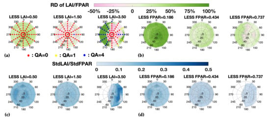
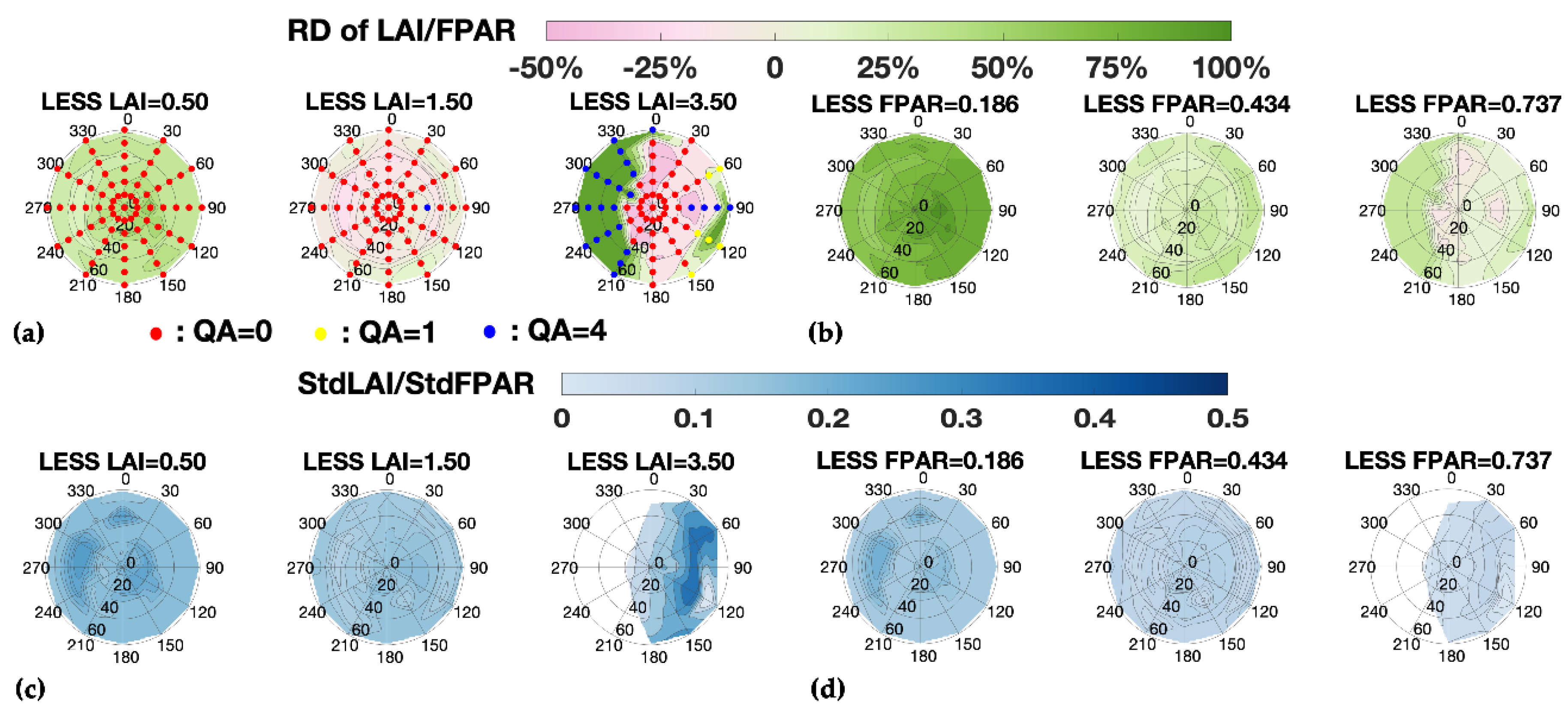
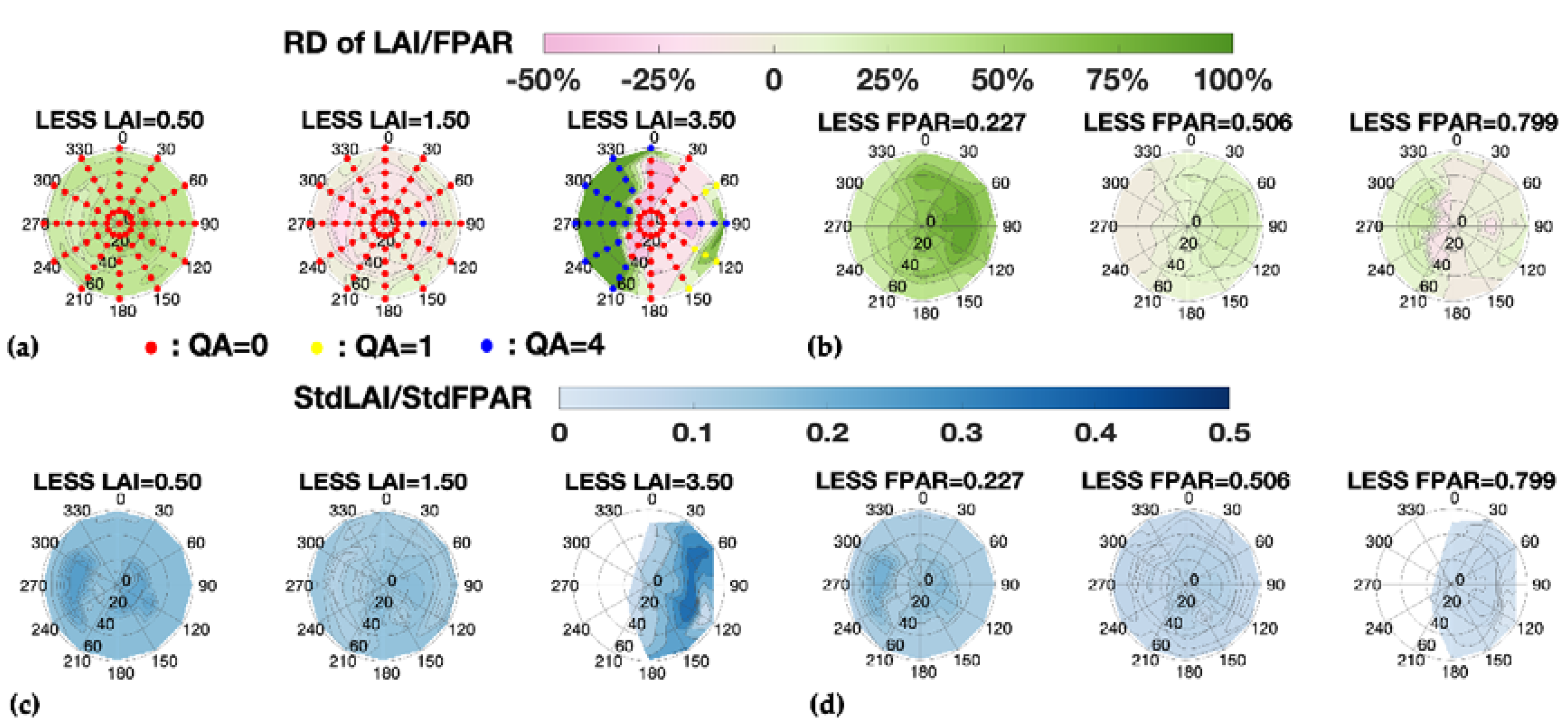
3.1.2. Retrieval Uncertainty as a Function of Sun–Sensor Geometry

The relationship between LAI/FPAR uncertainty and sun–sensor geometry are presented in Figure 4 and Figure 5. In the high LAI scene (Figure 4a, LAI = 3.50), the retrieval results of LAI/FPAR show low consistency with the truth (it yields to an overall uncertainty of 20.01% for RD of LAI and 13.96% for RD of FPAR). The main algorithm shows an averaged 6.61% underestimation of LAI, while the backup algorithm results in an averaged 84.85% overestimation of LAI. In this scene, the backup algorithm appears at the “hotspot” geometry and where the difference between SAA and VAA is large. It can also be seen that the large VZA will lead to saturation. Nevertheless, for the low LAI scene (LAI = 0.50), the retrieved LAI/FPAR showed a significant overestimation (+111.86% RD for LAI, +162.50% RD for FPAR) and large uncertainty (StdLAI = 0.285, and StdFPAR = 0.238). Figure 5 shows the same analysis as above, but we controlled the view position and varied the sun position. Comparing Figure 4 and Figure 5, the distribution of LAI and its uncertainty (Figure 4a,c, and Figure 5a,c) show higher consistency, while FPAR and its uncertainty (Figure 4b,d and Figure 5b,d) are slightly different.

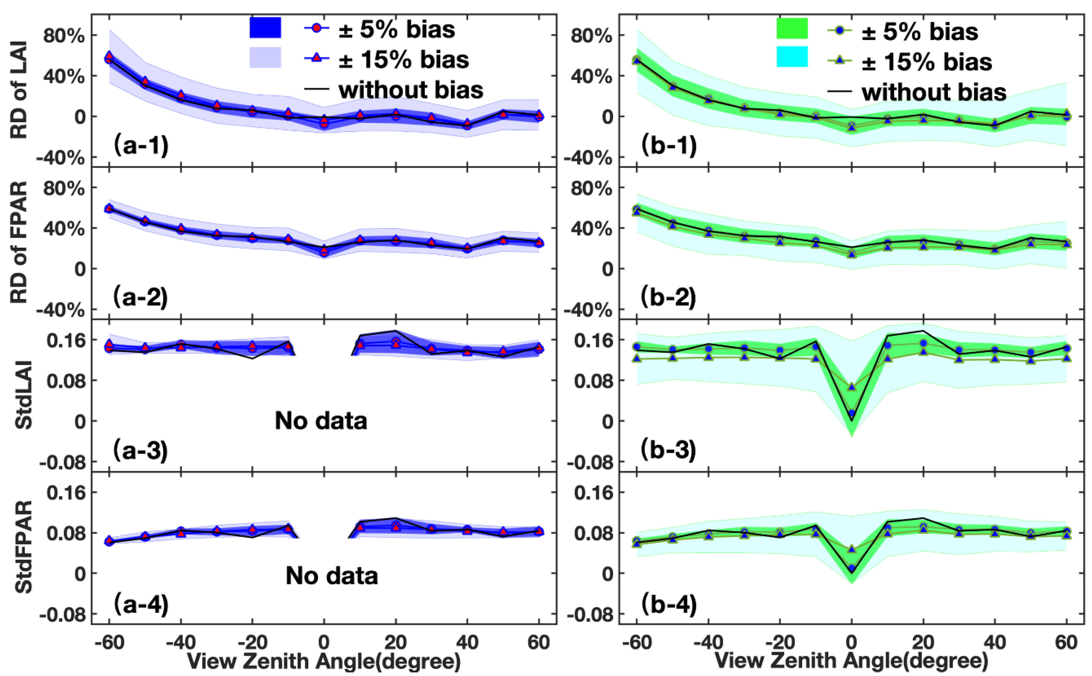
3.2. Input BRF Uncertainty

Here, we calculated the effects of input BRF uncertainty on the LAI/FPAR retrieval. Figure 6 shows that the uncertainty in the LAI/FPAR in the shadow area of the 15% BRF uncertainty is much larger, which means that larger BRF uncertainty will result in larger LAI/FPAR uncertainty. The StdLAI and StdFPAR due to a 5% BRF uncertainty are close to the StdLAI and StdFPAR due to a 15% BRF in the red band. This is because both 5% and 15% BRF uncertainty in the red band will trigger the backup algorithm with no StdLAI and StdFPAR. Comparing the shadow area in panels (a) and (b), we found that the same level of uncertainty in the NIR band BRF has a greater impact on the retrieval than the red band BRF. The main algorithm was not used in the hotspot (VZA = 0) geometry leading to the absence of both StdLAI and StdFPAR in panel (a).

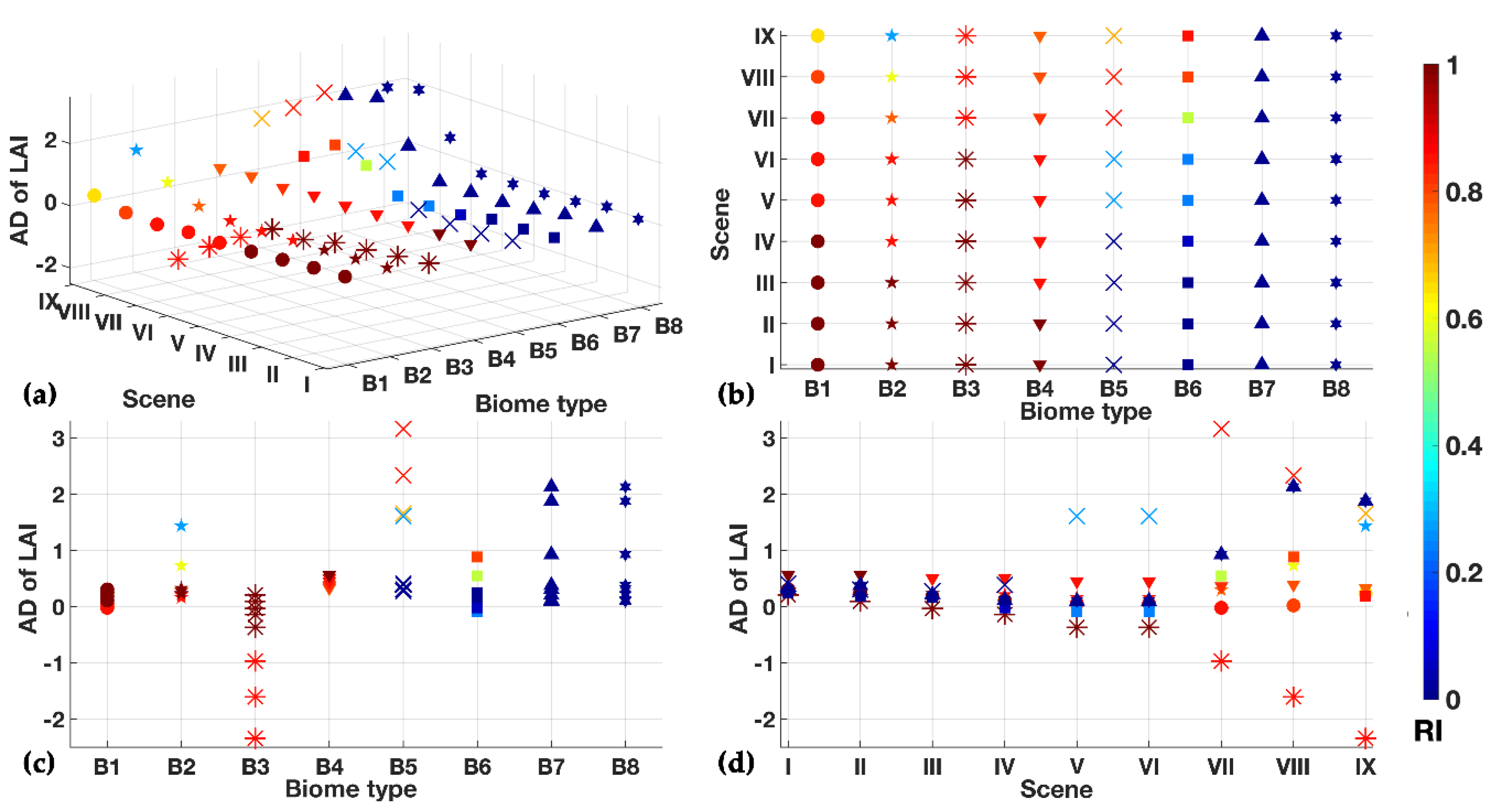
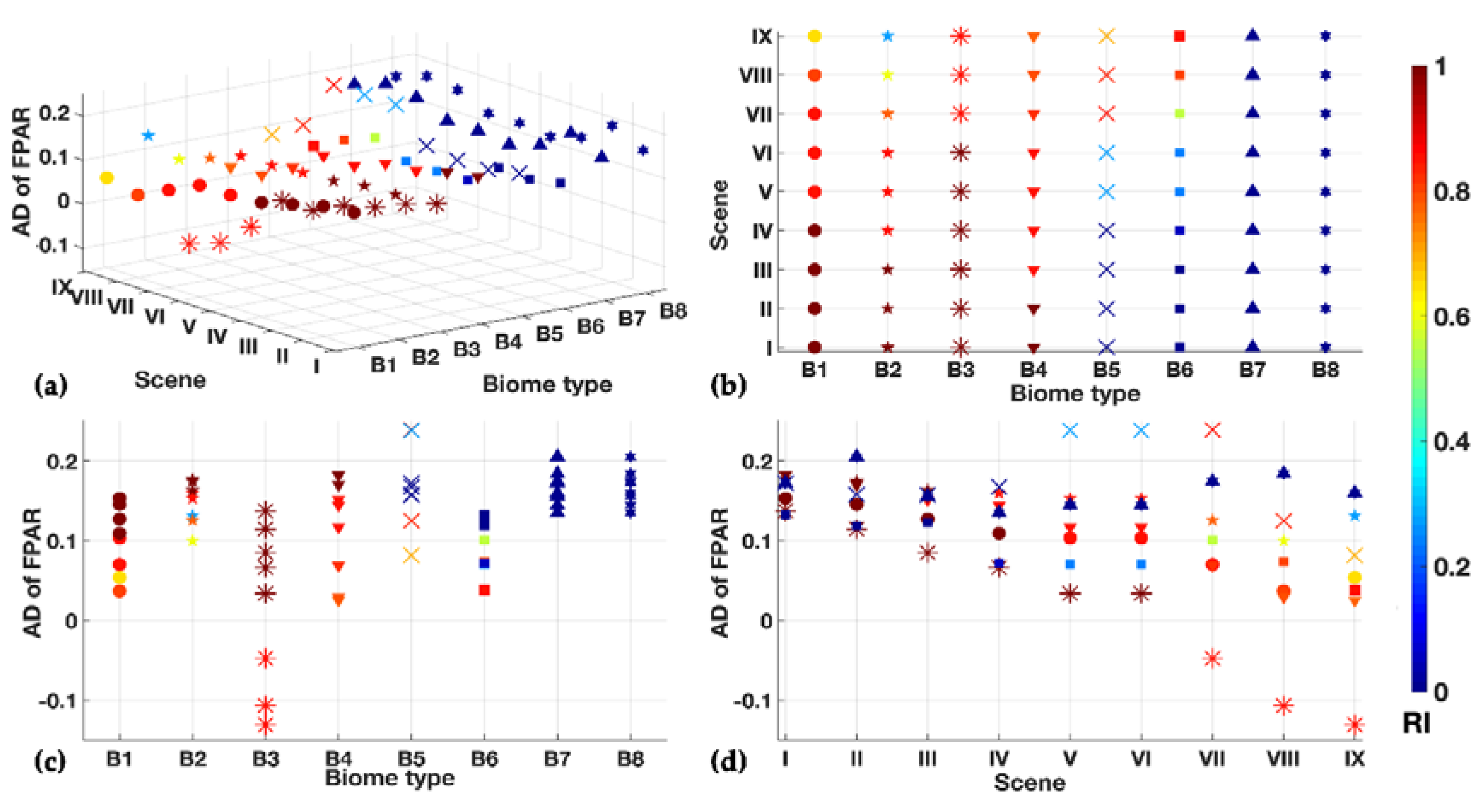
3.3. Input Biome Type Uncertainty

Different biome types have different canopy structures, and the MODIS retrieval algorithm uses photon transport theory and the corresponding RT model for different biome types to parameterize the canopy structures (e.g., reflectance and transmittance of leaves, crown shadowing), which form the LUTs of the MODIS retrieval algorithm. To check the sensitivity of the algorithm to biome type, we modified the input biome type for the retrieval algorithm from the correct type (B1: grasses and cereal crops) to incorrect types (B2: shrubs; B3: broadleaf crops; B4: savannas; B5: evergreen broadleaf forests; B6: deciduous broadleaf forests; B7: evergreen needleleaf forests; and B8: deciduous needleleaf forests). As seen from Figure 7 and Figure 8, the retrieval uncertainty is similar when the input biome types are non-forest biomes (B1-B4) with a greater than 59.5% RI for all four biome types except for B2 in the LAI = 4.5 scene. However, the RI gets much lower when the grassland pixel is misclassified into forest biomes. As shown in Figure 7c and Figure 8c, the uncertainties of the retrieved LAI are high at the scene with high LAI (e.g., LAI = 3.5, 4.5). A significant overestimation (+0.727, +1.434 for AD of LAI) in B2, and a significant underestimation (−1.608, −2.344 for AD of LAI) in B3 is also evident. For B5, the RI is high (>69%) but AD of LAI (>1.656) is also high when LAI is relatively high (e.g., LAI = 2.5, 3.5, 4.5). As shown in Figure 8c, the FPAR calculated from the MODIS algorithm is significantly overestimated for all cases except for B4 high LAI scenes, which appear to be underestimated.

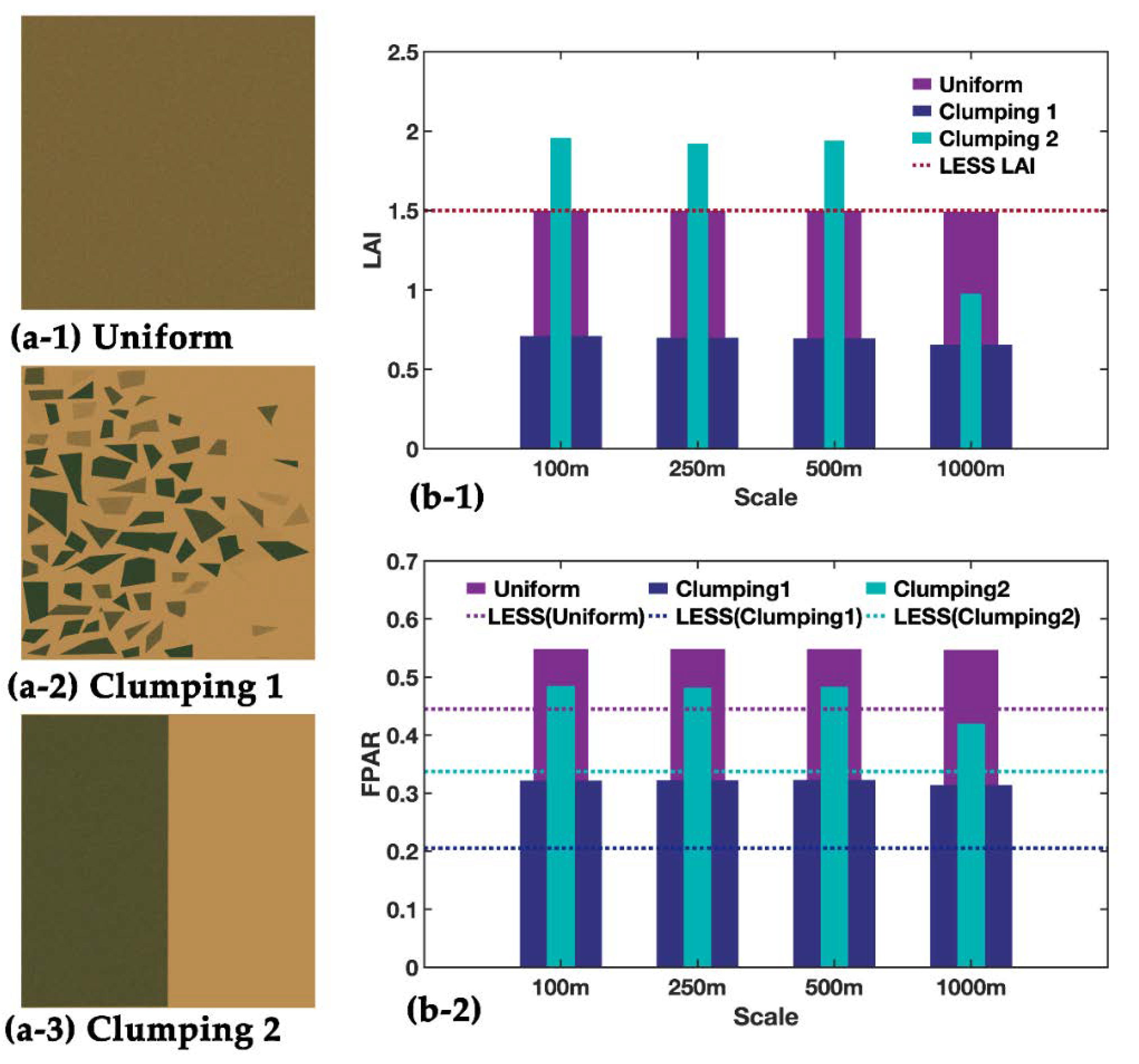
3.4. Impact of Clumping Effect and Scale Dependency

The model scale dependency and clumping effect have attracted much attention from the community in the development of quantitative remote sensing. In this experiment, the model scale dependency refers to the discrepancy between LAI/FPAR uncertainties that are derived from the same algorithm but at different spatial resolutions. The scale dependency determines the adaptive capacity of an algorithm for different pixel size. The clumping effect refers to the discrepancy between retrieved LAI/FPARs with same LAI/FPAR truth but different vegetation spatial distributions. The model nonlinearly and surface heterogeneity together result in the well-known phenomenon called “Inversion first and aggregation later is different from aggregation first and inversion later” [11].
Comparing the algorithm performance at different scales, we found that the MODIS algorithm is nearly scale-invariant from 100 m to 1000 m. Both LAI/FPAR and their uncertainty nearly remain unchanged with increasing pixel size except for the CT2, which shows that the StdLAI and StdFPAR are lower than other scales (Table 3). The retrieved LAIs for all scenes are less than the LAI truth at 1000 m scale, and the underestimations for Uniform, CT1, and CT2 vegetation distributions are −0.005, −0.846, and −0.525, respectively. Comparing the three clumping scenes, we found that the LAI of a uniform scene is very close to the LAI truth (Figure 9b-1). CT1 shows a significant underestimation, while CT2 shows a significant overestimation except in the 1000 m scale. For FPAR, there is a significant overestimation in all three scenes (Figure 9b-2). At the same spatial resolution, the RI of CT1 is the highest, followed by Uniform, and the lowest is CT2 (Table 3). While the values of StdLAI and StdFPAR are as follows (from small to large): Uniform, CT1, and CT2. The standard deviations of StdLAI and StdFPAR also get larger in this order.

4. Discussion

Because of the different sensitivities of LAI/FPAR to surface reflectances, we note that there would be a gap of uncertainty between the saturated part and the unsaturated part [4,8]. However, Figure 3 indicates that for large LAI/FPAR, their theoretical uncertainty is artificially reduced by the method of regularization, which causes the retrieval to have varying degrees of confidence and leads to a problematic evaluation of high LAI/FPAR scenes using the provided StdLAI and StdFPAR. This also places new requirements on future algorithm refinement that the LUT algorithm should be consistent in the saturated case as in the unsaturated case. The LAI/FPAR values estimated by the backup algorithm and calculated by the main algorithm also show significant discontinuity [4,8,9,10] (Figure 4a). Based on this, we point out that future algorithm refinement should increase the coverage of the main algorithm usage, which will greatly improve the overall accuracy of the product. In addition, according to the 3D RT model, the hotspot means that the radiation field tends to peak around the retro-illumination direction. The results of this study indicate that the uncertainty of the MODIS algorithm in the hotspots is quite large (Figure 4, Figure 5 and Figure 6), due to which the science team decided not to include additional hotspot parameters since their inclusion would make algorithm calibration difficult [56,57]. We note that this will not cause large problems in the MODIS LAI/FPAR production because of the fact that observations near the hotspot are rare for MODIS. However, this points out a new refinement direction of this algorithm to improve the accuracy of hotspot modeling for other sensors.
As is known, the uncertainty of the inputting BRFs has some influence on the uncertainty of the retrieval algorithm. In particular, our results show that the uncertainty of NIR BRFs has a larger effect on LAI/FPAR uncertainty compared to the red BRFs (Figure 6). We know that insufficient input information will lead to the “ill-posed” retrieval problem [11]; however, the inputting BRFs of the MODIS operational algorithm are currently only for the red and NIR bands. Therefore, in the future we may try to make use of BRFs in other bands to improve the retrieval accuracy. The MODIS algorithm depends on a priori information about the land surface given by biome type representing the pattern of the architecture of vegetation, as well as patterns of spectral reflectance and transmittance of vegetation [8]. Figure 7 and Figure 8 confirm that the misclassification of biome types with similar structures will result in smaller LAI/FPAR uncertainty, and vice versa [11,58]. This means that the improvement of biome classification accuracy is an efficient way to improve the LAI/FPAR products. Moreover, different biome types also lead to different clumping types. As Figure 9 shows, the underestimation of LAI is significant for two clumping scenes at 1000 m scale. For the other three scales, however, the overestimation of CT2 is due to the backup algorithm retrievals. As our results show, the algorithm only considers the clumping effect at one scale (e.g., B1 is minimal leaf clumping) [4], which can result in large differences in the retrievals; therefore, we suggest that future algorithms consider the clumping effect at more scales (e.g., leaf, branch, and crown).
We note that there are some problems with the way we use LESS to simulate specific scenes and evaluate the MODIS algorithm. First, according to the algorithm, the retrieved LAI/FPAR is a weighted average of the probability values within the error range. Therefore, the probability distribution of LAI/FPAR within the error range based on a great number of realizations has more statistical significance thus may differ from the specific realization (scene) that was used. Secondly, although the LESS model has been well validated, the confidence of our evaluation results depends on the accuracy of the LESS simulation.
In short, validation in the field of remote sensing utilizing computer simulations has proved feasible. In future studies, we will analyze the other seven biome types, which will provide a more comprehensive evaluation of the MODIS LAI/FPAR retrieval algorithm. In addition, we will change the mode of a single specific scene to obtain retrieval results by simulating multiple scenes. Moreover, evaluation of the algorithm at different levels of vegetation clumping will be the focus of our future research.

5. Conclusions

This paper presents an uncertainty assessment of the MODIS LAI/FPAR retrieval algorithm over B1 (grassland) based on computer simulation. To accomplish this assessment, we first analyzed the theoretical uncertainty caused by inherent model uncertainty, then we calculated the uncertainty caused by input parameters (BRF and biome type) over simulated 3D grass scenes. Finally, we analyzed the effects of vegetation clumping and scale dependency of the MODIS algorithm. The 3D grass scenes were simulated by a well validated 3D RT model (LESS), which helps to separate the model uncertainty and other uncertainties. We found that the uncertainty of the main and backup algorithm varies considerably. In the same scene, there is a −6.61% bias for the main algorithm retrieval, while the backup algorithm retrieval has a +84.85% bias. We noted that the uncertainty of the saturated retrievals is artificially reduced compared with unsaturated retrievals. At the same time, MODIS showed significant overestimation at low LAI scenes, with a maximum bias of +111.86% for LAI and +162.50% for FPAR. In the high LAI scenes, the “hotspot” geometry results in greater retrieval uncertainty from the backup algorithm. Moreover, input uncertainties further increased the uncertainty of LAI/FPAR retrieval. We found that the uncertainties in BRF in the NIR band has a greater impact than in the red band. The biome type uncertainty also leads to great retrieval uncertainty. Large uncertainties occurred when grassland was misclassified into forest biomes, while smaller uncertainties occurred when the misclassification was within the non-forest biomes. In addition, the clumping effect results in underestimation (−0.846 and −0.525 for the two clumping types, respectively) and we found that the MODIS algorithm is nearly scale-invariant from 100 m to 1000 m pixel sizes. Overall, these results, based on novel computer simulation experiments, can guide the future refinements of the MODIS LAI/FPAR algorithm.

Author Contributions

J.P.: formal analysis, writing—original draft preparation, investigation. K.Y.: conceptualization, methodology, writing—review and editing, funding acquisition, supervision, project administration. G.Z., Y.L., Y.Z., D.G., and H.L.: software, formal analysis. L.X.: writing—original draft preparation. Y.K. and R.B.M.: conceptualization, methodology. All authors have read and agreed to the published version of the manuscript.

Funding

This work was supported by the National Natural Science Foundation of China (41901298), the open fund of the State Key Laboratory of Remote Sensing Science (OFSLRSS201924), the open fund of the Key Laboratory of Digital Earth Science, the Institute of Remote Sensing and Digital Earth, the Chinese Academy of Sciences (2018LDE002), the Fundamental Research Funds for the Central Universities (2652018031) and the open fund of Shanxi Key Laboratory of Resources, Environment and Disaster Monitoring(2019-04).

Acknowledgments

We thank the MODIS LAI&FPAR team for all of their help and Jianbo Qi for support with the LESS 3D RT model. We also appreciate the fruitful suggestions from the anonymous reviewers which made the work better.

Conflicts of Interest

The authors declare no conflict of interest. The funders had no role in the design of the study; in the collection, analyses, or interpretation of data; in the writing of the manuscript, or in the decision to publish the results.

References

  1. Jacquemoud, S.; Baret, F.; Hanocq, J. Modeling spectral and bidirectional soil reflectance. Remote Sens. Environ. 1992, 41, 123–132. [Google Scholar] [CrossRef]
  2. Chen, J.M.; Black, T.A. Defining leaf area index for non-flat leaves. Plant Cell Environ. 1992, 15, 421–429. [Google Scholar] [CrossRef]
  3. GCOS. Systematic observation requirements for satellite-based products for climate. 2011 update supplemetnatl details to the satellite 39 based component og the implementation plan for the global observing system for climate in support of the unfccc (2010 update). In Technical Report; World Meteorological Organisation (WMO): Geneva, Switzerland, 2011. [Google Scholar]
  4. Knyazikhin, Y.; Martonchik, J.; Myneni, R.B.; Diner, D.; Running, S.W. Synergistic algorithm for estimating vegetation canopy leaf area index and fraction of absorbed photosynthetically active radiation from MODIS and MISR data. J. Geophys. Res. Atmos. 1998, 103, 32257–32275. [Google Scholar] [CrossRef] [Green Version]
  5. Sellers, P.; Dickinson, R.E.; Randall, D.; Betts, A.; Hall, F.; Berry, J.; Collatz, G.; Denning, A.; Mooney, H.; Nobre, C. Modeling the exchanges of energy, water, and carbon between continents and the atmosphere. Science 1997, 275, 502–509. [Google Scholar] [CrossRef] [PubMed] [Green Version]
  6. Zhu, Z.; Bi, J.; Pan, Y.; Ganguly, S.; Anav, A.; Xu, L.; Samanta, A.; Piao, S.; Nemani, R.R.; Myneni, R.B. Global data sets of vegetation leaf area index (LAI) 3g and fraction of photosynthetically active radiation (FPAR) 3g derived from global inventory modeling and mapping studies (GIMMS) normalized difference vegetation index (NDVI3g) for the period 1981 to 2011. Remote Sens. 2013, 5, 927–948. [Google Scholar]
  7. Mason, P.; Zillman, J.; Simmons, A.; Lindstrom, E.; Harrison, D.; Dolman, H.; Bojinski, S.; Fischer, A.; Latham, J.; Rasmussen, J. Implementation Plan for the Global Observing System for Climate in Support of the UNFCCC (2010 Update); World Meteorological Organization: Geneva, Switzerland, 2010; p. 180. [Google Scholar]
  8. Knyazikhin, Y. MODIS Leaf Area Index (LAI) and Fraction of Photosynthetically Active Radiation Absorbed by Vegetation (FPAR) Product (MOD 15) Algorithm Theoretical Basis Document. Available online: https://modis.gsfc.nasa.gov/data/atbd/atbd_mod15.pdf (accessed on 2 February 2017).
  9. Yan, K.; Park, T.; Yan, G.; Chen, C.; Yang, B.; Liu, Z.; Nemani, R.; Knyazikhin, Y.; Myneni, R. Evaluation of MODIS LAI/FPAR Product Collection 6. Part 1: Consistency and Improvements. Remote Sens. 2016, 8, 359. [Google Scholar] [CrossRef] [Green Version]
  10. Myneni, R.; Park, Y. MODIS Collection 6 (C6) LAI/FPAR Product User’s Guide. Available online: https://lpdaac.usgs.gov/sites/default/files/public/product_documentation/mod15_user_guide.pdf (accessed on 1 January 2016).
  11. Myneni, R.B.; Hoffman, S.; Knyazikhin, Y.; Privette, J.; Glassy, J.; Tian, Y.; Wang, Y.; Song, X.; Zhang, Y.; Smith, G. Global products of vegetation leaf area and fraction absorbed PAR from year one of MODIS data. Remote Sens. Environ. 2002, 83, 214–231. [Google Scholar] [CrossRef] [Green Version]
  12. Chen, L.; Dirmeyer, P.A. Adapting observationally based metrics of biogeophysical feedbacks from land cover/land use change to climate modeling. Environ. Res. Lett. 2016, 11, 034002. [Google Scholar] [CrossRef] [Green Version]
  13. Kala, J.; Decker, M.; Exbrayat, J.-F.; Pitman, A.J.; Carouge, C.; Evans, J.P.; Abramowitz, G.; Mocko, D. Influence of leaf area index prescriptions on simulations of heat, moisture, and carbon fluxes. J. Hydrometeorol. 2014, 15, 489–503. [Google Scholar] [CrossRef] [Green Version]
  14. Chen, C.; Park, T.; Wang, X.; Piao, S.; Xu, B.; Chaturvedi, R.K.; Fuchs, R.; Brovkin, V.; Ciais, P.; Fensholt, R.; et al. China and India lead in greening of the world through land-use management. Nat. Sustain. 2019, 2, 122–129. [Google Scholar] [CrossRef]
  15. Zhu, Z.; Piao, S.; Myneni, R.B.; Huang, M.; Zeng, Z.; Canadell, J.G.; Ciais, P.; Sitch, S.; Friedlingstein, P.; Arneth, A.; et al. Greening of the Earth and its drivers. Nat. Clim. Chang. 2016, 6, 791–795. [Google Scholar] [CrossRef]
  16. Zhang, Y.; Song, C.; Band, L.E.; Sun, G.; Li, J. Reanalysis of global terrestrial vegetation trends from MODIS products: Browning or greening? Remote Sens. Environ. 2017, 191, 145–155. [Google Scholar] [CrossRef] [Green Version]
  17. Baret, F.; Weiss, M.; Lacaze, R.; Camacho, F.; Makhmara, H.; Pacholcyzk, P.; Smets, B. GEOV1: LAI and FAPAR essential climate variables and FCOVER global time series capitalizing over existing products. Part1: Principles of development and production. Remote Sens. Environ. 2013, 137, 299–309. [Google Scholar] [CrossRef]
  18. Xiao, Z.; Liang, S.; Wang, J.; Chen, P.; Yin, X.; Zhang, L.; Song, J. Use of General Regression Neural Networks for Generating the GLASS Leaf Area Index Product From Time-Series MODIS Surface Reflectance. IEEE Trans. Geosci. Remote Sens. 2014, 52, 209–223. [Google Scholar] [CrossRef]
  19. Baret, F.; Buis, S. Estimating canopy characteristics from remote sensing observations: Review of methods and associated problems. In Advances in Land Remote Sensing; Springer: Berlin/Heidelberg, Germany, 2008; pp. 173–201. [Google Scholar]
  20. Claverie, M.; Vermote, E.F.; Weiss, M.; Baret, F.; Hagolle, O.; Demarez, V. Validation of coarse spatial resolution LAI and FAPAR time series over cropland in southwest France. Remote Sens. Environ. 2013, 139, 216–230. [Google Scholar] [CrossRef]
  21. Yan, K.; Park, T.; Chen, C.; Xu, B.; Song, W.; Yang, B.; Zeng, Y.; Liu, Z.; Yan, G.; Knyazikhin, Y.J.I.T.o.G.; et al. Generating global products of lai and fpar from snpp-viirs data: Theoretical background and implementation. IEEE Trans. Geosci. Remote Sens. 2018, 56, 2119–2137. [Google Scholar] [CrossRef]
  22. Serbin, S.P.; Ahl, D.E.; Gower, S.T. Spatial and temporal validation of the MODIS LAI and FPAR products across a boreal forest wildfire chronosequence. Remote Sens. Environ. 2013, 133, 71–84. [Google Scholar] [CrossRef]
  23. Fuster, B.; Sánchez-Zapero, J.; Camacho, F.; García-Santos, V.; Verger, A.; Lacaze, R.; Weiss, M.; Baret, F.; Smets, B. Quality Assessment of PROBA-V LAI, fAPAR and fCOVER Collection 300 m Products of Copernicus Global Land Service. Remote Sens. 2020, 12, 1017. [Google Scholar] [CrossRef] [Green Version]
  24. Weiss, M.; Baret, F.; Block, T.; Koetz, B.; Burini, A.; Scholze, B.; Lecharpentier, P.; Brockmann, C.; Fernandes, R.; Plummer, S. On Line Validation Exercise (OLIVE): A web based service for the validation of medium resolution land products. Application to FAPAR products. Remote Sens. 2014, 6, 4190–4216. [Google Scholar] [CrossRef] [Green Version]
  25. Yan, K.; Park, T.; Yan, G.; Liu, Z.; Yang, B.; Chen, C.; Nemani, R.; Knyazikhin, Y.; Myneni, R. Evaluation of MODIS LAI/FPAR Product Collection 6. Part 2: Validation and Intercomparison. Remote Sens. 2016, 8, 460. [Google Scholar] [CrossRef] [Green Version]
  26. De Kauwe, M.G.; Disney, M.; Quaife, T.; Lewis, P.; Williams, M. An assessment of the MODIS collection 5 leaf area index product for a region of mixed coniferous forest. Remote Sens. Environ. 2011, 115, 767–780. [Google Scholar] [CrossRef]
  27. Loew, A.; Bell, W.; Brocca, L.; Bulgin, C.E.; Burdanowitz, J.; Calbet, X.; Donner, R.V.; Ghent, D.; Gruber, A.; Kaminski, T. Validation practices for satellite based earth observation data across communities. Rev. Geophys. 2017, 55, 779–817. [Google Scholar] [CrossRef] [Green Version]
  28. Fang, H.; Baret, F.; Plummer, S.; Schaepman-Strub, G. An overview of global leaf area index (LAI): Methods, products, validation, and applications. Rev. Geophys. 2019, 57, 739–799. [Google Scholar] [CrossRef]
  29. Fang, H.; Wei, S.; Liang, S. Validation of MODIS and CYCLOPES LAI products using global field measurement data. Remote Sens. Environ. 2012, 119, 43–54. [Google Scholar] [CrossRef]
  30. Somers, B.; Tits, L.; Coppin, P. Quantifying Nonlinear Spectral Mixing in Vegetated Areas: Computer Simulation Model Validation and First Results. IEEE J. Sel. Top. Appl. Earth Observ. Remote Sens. 2014, 7, 1956–1965. [Google Scholar] [CrossRef]
  31. Schneider, F.D.; Leiterer, R.; Morsdorf, F.; Gastelluetchegorry, J.P.; Lauret, N.; Pfeifer, N.; Schaepman, M.E. Simulating imaging spectrometer data: 3D forest modeling based on LiDAR and in situ data. Remote Sens. Environ. 2014, 152, 235–250. [Google Scholar] [CrossRef]
  32. Lanconelli, C.; Gobron, N.; Adams, J.; Danne, O.; Blessing, S.; Robustelli, M.; Kharbouche, S.; Muller, J. Report on the Quality Assessment of Land ECV Retrieval Algorithms; Scientific and Technical Report JRC109764; European Commission, Joint Research Centre: Ispra, Italy, 2018. [Google Scholar]
  33. Gastellu-Etchegorry, J.-P.; Yin, T.; Lauret, N.; Cajgfinger, T.; Gregoire, T.; Grau, E.; Feret, J.-B.; Lopes, M.; Guilleux, J.; Dedieu, G. Discrete anisotropic radiative transfer (DART 5) for modeling airborne and satellite spectroradiometer and LIDAR acquisitions of natural and urban landscapes. Remote Sens. 2015, 7, 1667–1701. [Google Scholar] [CrossRef] [Green Version]
  34. Huang, H.; Qin, W.; Liu, Q. RAPID: A Radiosity Applicable to Porous IndiviDual Objects for directional reflectance over complex vegetated scenes. Remote Sens. Environ. 2013, 132, 221–237. [Google Scholar] [CrossRef]
  35. Qi, J.; Xie, D.; Yin, T.; Yan, G.; Gastellu-Etchegorry, J.-P.; Li, L.; Zhang, W.; Mu, X.; Norford, L.K. LESS: LargE-Scale remote sensing data and image simulation framework over heterogeneous 3D scenes. Remote Sens. Environ. 2019, 221, 695–706. [Google Scholar] [CrossRef]
  36. Widlowski, J.L.; Pinty, B.; Lopatka, M.; Atzberger, C.; Buzica, D.; Chelle, M.; Disney, M.; Gastelluetchegorry, J.; Gerboles, M.; Gobron, N. The fourth radiation transfer model intercomparison (RAMI-IV): Proficiency testing of canopy reflectance models with ISO-13528. J. Geophys. Res. 2013, 118, 6869–6890. [Google Scholar] [CrossRef] [Green Version]
  37. Disney, M.; Lewis, P.; Saich, P. 3D modelling of forest canopy structure for remote sensing simulations in the optical and microwave domains. Remote Sens. Environ. 2006, 100, 114–132. [Google Scholar] [CrossRef]
  38. Widlowski, J.-L.; Côté, J.-F.; Béland, M. Abstract tree crowns in 3D radiative transfer models: Impact on simulated open-canopy reflectances. Remote Sens. Environ. 2014, 142, 155–175. [Google Scholar] [CrossRef]
  39. Kuusk, A. 3.03—Canopy Radiative Transfer Modeling. In Comprehensive Remote Sensing; Liang, S., Ed.; Elsevier: Oxford, UK, 2018; pp. 9–22. [Google Scholar] [CrossRef]
  40. Gastelluetchegorry, J.P.; Martin, E.; Gascon, F. DART: A 3D model for simulating satellite images and studying surface radiation budget. Int. J. Remote Sens. 2004, 25, 73–96. [Google Scholar] [CrossRef]
  41. Bruniquelpinel, V.; Gastelluetchegorry, J.P. Sensitivity of Texture of High Resolution Images of Forest to Biophysical and Acquisition Parameters. Remote Sens. Environ. 1998, 65, 61–85. [Google Scholar] [CrossRef]
  42. Guillevic, P.; Gastellu-Etchegorry, J. Modeling BRF and radiative regime of tropical and boreal forests—PART II: PAR regime. Remote Sens. Environ. 1999, 68, 317–340. [Google Scholar] [CrossRef]
  43. Demarez, V.; Gastelluetchegorry, J.P. A Modeling Approach for Studying Forest Chlorophyll Content. Remote Sens. Environ. 2000, 71, 226–238. [Google Scholar] [CrossRef]
  44. Malenovsky, Z.; Homolova, L.; Zuritamilla, R.; Lukes, P.; Kaplan, V.; Hanus, J.; Gastelluetchegorry, J.P.; Schaepman, M.E. Retrieval of spruce leaf chlorophyll content from airborne image data using continuum removal and radiative transfer. Remote Sens. Environ. 2013, 131, 85–102. [Google Scholar] [CrossRef] [Green Version]
  45. Qi, J.; Xie, D.; Yan, G.; Gastelluetchegorry, J.P. Simulating Spectral Images with Less Model Through a Voxel-Based Parameterization of Airborne Lidar Data. In Proceedings of the International Geoscience and Remote Sensing Symposium, Yokohama, Japan, 28 July–2 August 2019; pp. 6043–6046. [Google Scholar]
  46. Qi, J.; Xie, D.; Guo, D.; Yan, G. A Large-Scale Emulation System for Realistic Three-Dimensional (3-D) Forest Simulation. IEEE J. Sel. Top. Appl. Earth Observ. Remote Sens. 2017, 10, 4834–4843. [Google Scholar] [CrossRef]
  47. Huang, D.; Knyazikhin, Y.; Wang, W.; Deering, D.W.; Stenberg, P.; Shabanov, N.V.; Tan, B.; Myneni, R.B. Stochastic transport theory for investigating the three-dimensional canopy structure from space measurements. Remote Sens. Environ. 2008, 112, 35–50. [Google Scholar] [CrossRef]
  48. Yang, B.; Knyazikhin, Y.; Mottus, M.; Rautiainen, M.; Stenberg, P.; Yan, L.; Chen, C.; Yan, K.; Choi, S.; Park, T. Estimation of leaf area index and its sunlit portion from DSCOVR EPIC data: Theoretical basis. Remote Sens. Environ. 2017, 198, 69–84. [Google Scholar] [CrossRef] [Green Version]
  49. Yang, W.; Tan, B.; Huang, D.; Rautiainen, M.; Shabanov, N.V.; Wang, Y.; Privette, J.L.; Huemmrich, K.F.; Fensholt, R.; Sandholt, I. MODIS leaf area index products: From validation to algorithm improvement. IEEE Trans. Geosci. Remote Sens. 2006, 44, 1885–1898. [Google Scholar] [CrossRef]
  50. Hosgood, B.; Jacquemoud, S.; Andreoli, G.; Verdebout, J.; Pedrini, G.; Schmuck, G. Leaf optical properties experiment 93 (LOPEX93). Rep. Eur. 1995, 16095. [Google Scholar]
  51. Trigg, S.; Flasse, S. Characterizing the spectral-temporal response of burned savannah using in situ spectroradiometry and infrared thermometry. Int. J. Remote Sens. 2000, 21, 3161–3168. [Google Scholar] [CrossRef]
  52. Fang, H.; Jiang, C.; Li, W.; Wei, S.; Baret, F.; Chen, J.M.; Garcia-Haro, J.; Liang, S.; Liu, R.; Myneni, R.B.; et al. Characterization and intercomparison of global moderate resolution leaf area index (LAI) products: Analysis of climatologies and theoretical uncertainties. J. Geophys. Res. 2013, 118, 529–548. [Google Scholar] [CrossRef]
  53. Xu, B.; Park, T.; Yan, K.; Chen, C.; Zeng, Y.; Song, W.; Yin, G.; Li, J.; Liu, Q.; Knyazikhin, Y.; et al. Analysis of Global LAI/FPAR Products from VIIRS and MODIS Sensors for Spatio-Temporal Consistency and Uncertainty from 2012–2016. Forests 2018, 9, 73. [Google Scholar] [CrossRef] [Green Version]
  54. Knyazikhin, Y.; Martonchik, J.V.; Diner, D.J.; Myneni, R.B.; Verstraete, M.M.; Pinty, B.; Gobron, N. Estimation of vegetation canopy leaf area index and fraction of absorbed photosynthetically active radiation from atmosphere-corrected MISR data. J. Geophys. Res. 1998, 103, 32239–32256. [Google Scholar] [CrossRef] [Green Version]
  55. Chen, J.M.; Leblanc, S.G. A four-scale bidirectional reflectance model based on canopy architecture. IEEE Trans. Geosci. Remote Sens. 1997, 35, 1316–1337. [Google Scholar] [CrossRef]
  56. Kuusk, A. The hot spot effect on a uniform vegetative cover. Sov. J. Remote Sens 1985, 3, 645–658. [Google Scholar]
  57. Roujean, J.-L. A parametric hot spot model for optical remote sensing applications. Remote Sens. Environ. 2000, 71, 197–206. [Google Scholar] [CrossRef]
  58. Myneni, R.B.; Ramakrishna, R.; Nemani, R.R.; Running, S.W. Estimation of global leaf area index and absorbed par using radiative transfer models. IEEE Trans. Geosci. Remote Sens. 1997, 35, 1380–1393. [Google Scholar] [CrossRef] [Green Version]
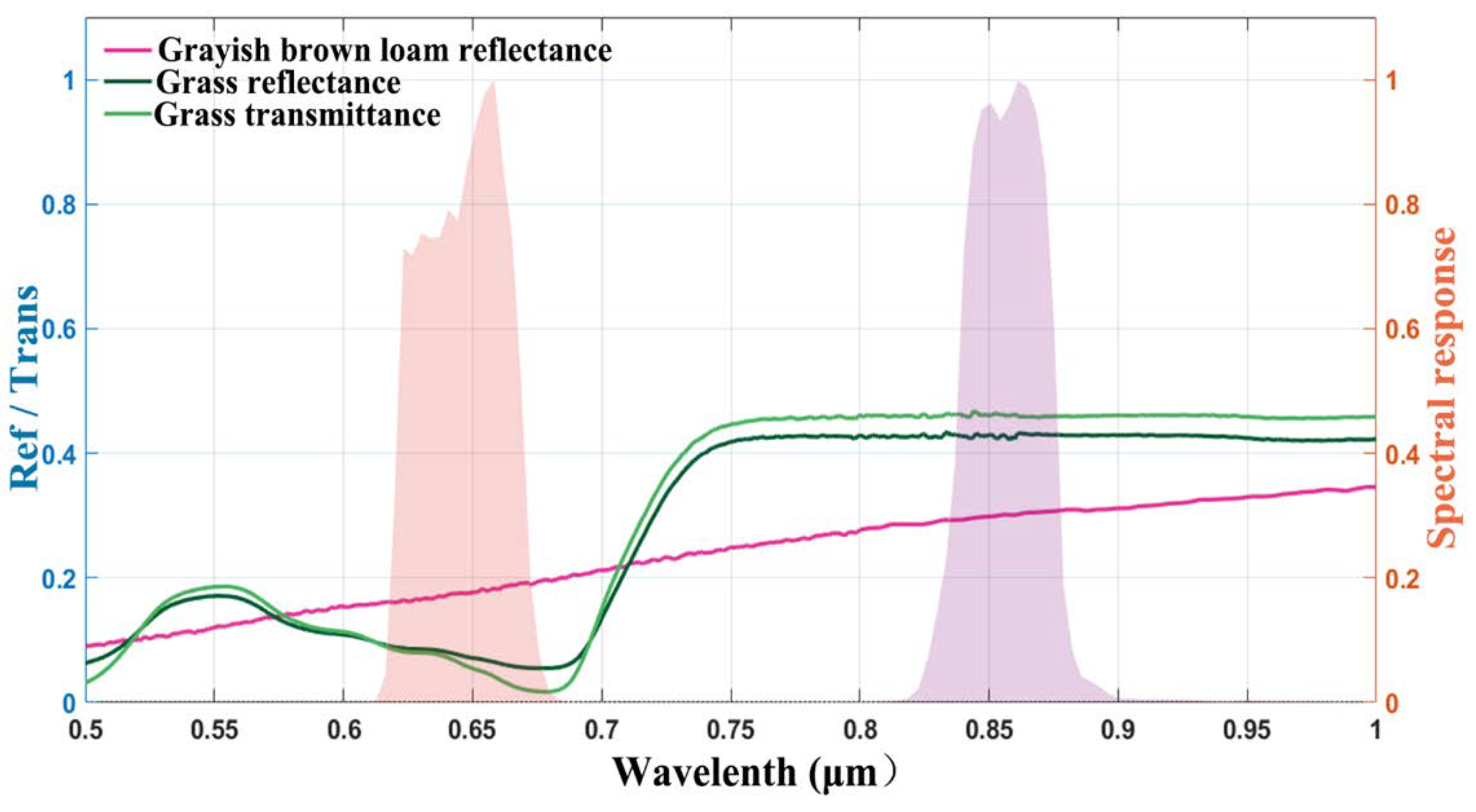
Figure 1. Variation of reflectance (Ref), transmittance (Trans), and spectral response function (SRF) values at different wavelengths. The dark green and magenta curves represent the grass and soil reflectances, and the light green represents the grass transmittance. The shades of red and purple represent the SRFs of the MODIS sensor in the red (620–670 μ m ) and NIR (841–876 μ m ) bands, respectively.
Remotesensing 12 03391 g001
Figure 2. Simulated scenes with nine different LAI values using the LESS 3D RT model. Panels (a)–(i) are with LAI = 0.25, 0.50, 0.75, 1.0, 1.25, 1.5, 2.5, 3.5, and 4.5, respectively. The plots represent a smaller portion (5 m × 5 m) of a 500 m × 500 m scene. The grasses are randomly distributed in these scenes.
Remotesensing 12 03391 g002
Figure 3. Distribution of LAI/FPAR values and associated uncertainty derived from the main RT-based algorithm in the red-NIR space. The SZA, SAA, VZA, and VAA were all fixed at 0°. Panel (ae) represent the retrieved LAI, FPAR, algorithm path (QA = 0: main algorithm without saturation, QA = 1: main algorithm with saturation), StdLAI, and StdFPAR, respectively.
Remotesensing 12 03391 g003
Figure 4. The uncertainty (LAI/FPAR RD, StdLAI, and StdFPAR) as a function of sensor geometry when the SZA is 30° and SAA is 90°. (a)–(d) are RD of LAI, RD of FPAR, StdLAI, and StdFPAR in three different scenes (Scene 1: LAI = 0.50 and FPAR = 0.186, Scene 2: LAI = 1.50 and FPAR = 0.434, Scene 3: LAI = 3.50 and FPAR = 0.737), respectively. The colored dots in panel (a) represent different algorithm paths (main without saturated: QA = 0, main with saturated: QA = 1, backup: QA = 4).
Remotesensing 12 03391 g004
Figure 5. The LAI/FPAR uncertainty as a function of sun geometry. Same as Figure 4 but for sun geometry and the VZA is 30° and VAA is 90°. The FPAR values of the scenes are calculated as the mean of different solar angles.
Remotesensing 12 03391 g005
Figure 6. LAI/FPAR uncertainty caused by input BRF uncertainty as a function of the view zenith angle (VZA). Panel (a) and panel (b) represent the red and NIR band, respectively. The LAI value of the scene is 1.5, and the SZA, SAA and VAA are all set to 0. The upper two panels show the RD of LAI/FPAR and the lower two panels show the StdLAI and StdFPAR, respectively. Dots are the mean values of LAI/FPAR calculated by 1000 different BRFs and shadow indicates the standard deviation of these retrievals. “No data” means that RI is equal to 0 and neither StdLAI nor StdFPAR exists in this VZA condition.
Remotesensing 12 03391 g006
Figure 7. Illustration of the retrieval index (RI, indicated by different colors) and the absolute difference (AD) of LAI as a function of biome type and different scenes. Panel (b) and (d) are the x–z (x means biome type and z means AD) sections of the panel (a) and (c), respectively, which show the approximate range of AD of LAI in different biome types. Scenes I to IX represent the LAI truth being equal to 0.25, 0.5, 0.75, 1.00, 1.25, 1.50, 2.50, 3.50, and 4.50, respectively. The colors in the figure are the values of RI. The eight biome types are: grasses and cereal crops (B1); shrubs (B2); broadleaf crops (B3); savannas (B4); evergreen broadleaf forests (B5); deciduous broadleaf forests (B6); evergreen needleleaf forests (B7); and deciduous needleleaf forests (B8), where B1 is the correct input, and B2–B8 all represent misclassification. The shapes of the different symbols correspond to different biome types (one by one in panel (b) and (c)).
Remotesensing 12 03391 g007
Figure 8. Illustration of the RI and the AD of FPAR as a function of biome type and different scenes. Same as Figure 7 but for FPAR.
Remotesensing 12 03391 g008
Figure 9. Comparison of LAI/FPAR retrievals over different clumping scenes and scales. Panel (a) is for three 1 km2 scenes (a-1: uniform, a-2: randomly generated clumping (CT1), a-3: half-and-half clumping (CT2)) and panel (b) shows the retrievals over three different scenes and four different scales (100 m, 250 m, 500 m, and 1000 m) where the dashed line represents the LAI/FPAR truth.
Remotesensing 12 03391 g009
Table 1. Broad-band reflectance and transmittance of grass and soil used in this study. R and T are abbreviations for broad-band reflectance and transmittance, respectively.
R (Red)T (Red)R (NIR)T (NIR)
Johnson grass0.07380.05770.42760.4607
Grayish brown loam0.175500.30210
Table 2. Parameter configuration for designed experiments. SZA, SAA, VZA, VAA means solar zenith angle, solar azimuth angle, view zenith angle, and view azimuth angle, respectively.
ExperimentLAISZASAAVZAVAAUncertainty Metrics
Retrieval Space/StdLAI, StdFPAR
Sun–Sensor Geometry0.50, 1.5, 3.530°/
0°:10°:60°
90°/
0°:30°:330°
0°:10°:60°/30°0°:30°:330°/
90°
RD, StdLAI, StdFPAR
BRF Uncertainty1.5−60°:10°:60°RD, StdLAI, StdFPAR
Biome Type Uncertainty0.25, 0.50, 0.75, 1.0, 1.25, 1.5, 2.5, 3.5, 4.50°:10°:60°0°:30°:330°RI, AD
Clumping and Scale Effect1.530°0°:30°:60°0°:60°:300°RI, StdLAI, StdFPAR
Table 3. The uncertainty metrics of three different clumping scenes and four scales.
Scene100 m250 m500 m1000 m
RI
(N. of main/N. of all)
Uniform1700/1800272/28868/7217/18
CT11743/1800279/28870/7218/18
CT21565/1800251/28862/7217/18
StdLAI
(mean ± Std)
Uniform0.147±
0.019
0.148±
0.019
0.149±
0.020
0.150±
0.021
CT10.251±
0.108
0.218±
0.074
0.225±
0.066
0.179±
0.074
CT20.340±
0.160
0.339±
0.160
0.342±
0.159
0.181±
0.027
StdFPAR
(mean ± Std)
Uniform0.088±
0.012
0.088±
0.012
0.089±
0.012
0.089±
0.013
CT10.208±
0.109
0.177±
0.070
0.180±
0.058
0.144±
0.061
CT20.269±
0.188
0.269±
0.188
0.271±
0.187
0.130±
0.022
Publisher’s Note: MDPI stays neutral with regard to jurisdictional claims in published maps and institutional affiliations.

