Article

Analyzing Ecological Vulnerability and Vegetation Phenology Response Using NDVI Time Series Data and the BFAST Algorithm

1
College of Land Science and Technology, China Agricultural University, Beijing 100083, China
2
Key Laboratory for Agricultural Land Quality Monitoring and Control, Ministry of Natural Resources, Beijing 100035, China
3
Land Consolidation and Rehabilitation Center, Ministry of Natural Resources of the People’s Republic of China, Beijing 100035, China
*
Author to whom correspondence should be addressed.
Remote Sens. 2020, 12(20), 3371; https://doi.org/10.3390/rs12203371
Submission received: 7 September 2020 / Revised: 1 October 2020 / Accepted: 13 October 2020 / Published: 15 October 2020
(This article belongs to the Special Issue Remote Sensing in Support of Environmental Governance)

Abstract

:
Identifying ecologically vulnerable areas and understanding the responses of phenology to negative changes in vegetation growth are important bases for ecological restoration. However, identifying ecologically vulnerable areas is difficult because it requires high spatial resolution and dense temporal resolution data over a long time period. In this study, a novel method is presented to identify ecologically vulnerable areas based on the normalized difference vegetation index (NDVI) time series from MOD09A1. Here, ecologically vulnerable areas are defined as those that experienced negative changes frequently and greatly in vegetation growth after the disturbances during 2000–2018. The number and magnitude of negative changes detected by the Breaks for Additive Season and Trend (BFAST) algorithm based on the NDVI time-series data were combined to identify ecologically vulnerable areas. TIMESAT was then used to extract the phenology metrics from an NDVI time series dataset to characterize the vegetation responses due to the abrupt negative changes detected by the BFAST algorithm. Focus was given to Jilin Province, a region of China known to be ecologically vulnerable because of frequent drought. The results showed that 13.52% of the study area, mostly in Jilin Province, is ecologically vulnerable. The vulnerability of trees is the lowest, while that of sparse vegetation is the highest. The response of phenology is such that the relative amount of vegetation biomass and length of the growing period were decreased by negative changes in growth for dense vegetation types. The present research results will be useful for the protection of environments being disturbed by regional ecological restoration.

Graphical Abstract

1. Introduction

Frequent natural disasters and the irrational exploitation of natural resources by human beings have led to a gradual increase in ecosystem vulnerability [1,2,3,4]. The definition of vulnerability by Turner et al. is the degree to which a system, subsystem, or system component is likely to experience harm due to exposure to a hazard, either a perturbation or a stress [5]. In other words, compared with ecologically stable areas, the normal functions and structures of an ecosystem in vulnerable areas are more susceptible to damage. Finally, this damage may subsequently trigger a chain of responses leading to the loss of species diversity and a decline in land productivity in vulnerable areas [6]. Consequently, identifying ecologically vulnerable areas has become the first step in ecosystem restoration projects. Negative changes in vegetation growth are an early sign of environmental degradation [7]. Vegetation phenology is often considered the “leading indicator” of ecological responses to environmental changes [8]. Most studies on environmental changes are directed at land use/land cover (LULC) [9]. However, the relationship between negative changes in vegetation growth and phenology remain largely unexplored [10]. Identifying the phenological responses corresponding to negative changes in vegetation growth will be helpful in understanding the process of vegetation restoration and reconstruction.
According to the definition of vulnerability by Turner et al. [5], vulnerability is characterized by instability and sensitivity to disturbances [11]. “Stable” means that ecosystem changes, during a defined period of time, remain constant, oscillate, reach a fixed point, or present some other type of behavior [12]. Sensitivity is the magnitude of the stressing event that the system will resist or absorb without significant change [13]. Thus, the areas where ecosystems are most unstable and sensitive to disturbances are defined as ecologically vulnerable areas. Vegetation growth is a direct and obvious indicator that describes the condition of the ecosystems experiencing disturbances [14]. Vegetation growth is suddenly disrupted—an abrupt change—when an ecosystem is subjected to an extreme disturbance beyond its tolerance threshold [15]. The Ministry of Environmental Protection of China noted in the “National Plan for the Protection of Ecologically Vulnerable Areas” that ecologically vulnerable areas manifest a decline in biological productivity, are sensitive to environmental changes, and exhibit significant inter-annual changes in time [16]. Jiang et al. used abrupt negative changes in vegetation to evaluate the ecological adaptive capacity under drought [17]. Therefore, abrupt changes in vegetation could be used to evaluate ecosystem instability and sensitivity, which are the key features for evaluating vulnerability in response to disturbances. In this paper, ecologically vulnerable areas were identified through instability and sensitivity based on abrupt negative changes in vegetation growth. The number and magnitude of abrupt negative changes in vegetation indicate instability and sensitivity, respectively. Therefore, areas featuring frequent and significant abrupt negative changes in vegetation growth after disturbances during the monitoring period are considered to be ecologically vulnerable areas. Research on phenological changes mainly focuses on climate change and phenological influence, while the phenological changes from abrupt negative changes in vegetation growth have rarely been explored [18,19]. Phenological changes in vegetation experiencing negative changes helps explain the feedback mechanism of vegetation in response to disturbances, from which a theoretical basis for ecological resilience research is also provided [20,21].
Remote sensing (RS) imaging allows for wider spatial coverage and access to a broader archive of historical imagery. The detection of abrupt changes in vegetation involves extracting breakpoints in time-series trajectories from multitemporal satellite RS imagery. It is applied to detect abrupt changes in vegetation caused by disturbances, including human activities and natural events [22], such as fire [23], deforestation [24], droughts [25], and floods [26]. MODIS data are considered an excellent data source in region vegetation dynamic research because they provide 21 years of accumulated data with both high temporal resolution and moderate spatial resolution [27,28,29]. NDVI time series have been applied to analyze vegetation growth history [30], monitor current growth conditions [31], and predict future vegetation dynamics [32]. Some researchers have proven that the breakpoints of NDVI are caused by environmental disturbances. For example, disturbances, such as droughts, floods, and fires, are in line with the negative changes at NDVI breakpoints [22,33,34]. The definitions of the ecosystem or environmental disturbances are often taken from White and Picket (1985), who describe a disturbance as any relatively discrete event that disrupts the structure of an ecosystem, community, or population and changes resource availability or the physical environment [35]. It can be inferred that, at the breakpoint, a negative change in the NDVI time series indicates that the vegetation has been disturbed. The BFAST algorithm detects and identifies the timing and magnitude of breaks in an NDVI time series, which, in turn, can be used to screen areas with frequent and abrupt negative changes and, consequently, identify ecologically vulnerable areas. Several methods have been proposed to detect abrupt changes in vegetation, such as the Landsat-based Detection of Trends in Disturbance and Recovery (LandTrendr) [36], the Breaks for Additive Season and Trend (BFAST) algorithm [37], the Vegetation Change Tracker (VCT) [38], and the Detecting Breakpoints and Estimating Segments in Trend (DBEST) method [39]. The BFAST algorithm, developed by Versbesselt et al. in 2010, is used to identify the breakpoints of the trend components and seasonal components in NDVI time series [40]. With BFAST, high-precision data (with each pixel in the time series fitted individually) can be analyzed without setting a threshold, while detailed information, including the number, time, and magnitude of changes, are estimated. BFAST has been applied to monitor vegetation changes caused by deforestation, forest disturbances, and restoration [41,42]. Considering the phenological parameters of NDVI and trajectory characteristics, some packages, such as HANTS [43], TiSeG [44], TSPT [45], and TIMESAT [46], were developed to extract phenological information. Among the proposed packages, the TIMESAT software package is applied to parameterize the phenological and temporal behavior of NDVI on a seasonal scale. This package integrates a series of filter functions and extraction methods for extracting phenological information, which extract phenological information according to different land types. TIMESAT was developed to generate several seasonal data by fitting a smooth model function to the upper envelope of the RS time-series data. There are three different curve-fitting models: Savitzky–Golay (SG) filtering, asymmetric Gaussian (AG), and double logistic (DL). The SG model has been successfully used for the extraction of phenological parameters due to its high fitting accuracy [47]. In this paper, TIMESAT is used to extract the phenological indicators of different vegetation types.
It is necessary to develop a method for identifying vulnerable areas based on negative changes in vegetation growth and to explore the response mechanisms of the phenology to negative changes. The objectives of this study were (1) to identify areas where the number of negative changes is greater than 0 and the change direction is negative in vegetation growth from the NDVI time series trajectory extracted by the BFAST algorithm in Jilin Province, China during 2000–2018; (2) to compare the stability and sensitivity of different vegetation types; and (3) to explore the response mechanism of the phenology to negative changes by analyzing the relationship between the phenological indicators extracted by TIMESAT and the negative changes decomposed by BFAST.

2. Materials and Methods

2.1. Study Area

Jilin Province is located in the northeast of China (121°38′–131°19′ E, 40°50′–46°19′ N) and covers an area of approximately 18.74 × 10⁴ km2. The topography in Jilin Province is rugged in the east and smooth in the west. The terrain is divided into the southeast Changbai Mountains and the northwest Songliao Plain, taking the Dahei Mountains as the boundary, as shown in the LULC map. The study area has a temperate continental monsoon climate. From the southeast to the northwest, the climate transitions from a humid climate to a semi-humid climate and then to a semi-arid climate. The annual total precipitation forms a southeast–northwest gradient, decreasing from 800 to 400 mm. The annual evapotranspiration increases from 1200 to 1800 mm, and the mean temperature decreases from 7 to 3 °C. The climate in the eastern region is humid and rainy, where the annual precipitation is 650 mm. The western part is dry, where the annual precipitation is below 500 mm. The average wind speed is 3.4–3.8 m/s. The natural vegetation of the Jilin Province has been intensively disturbed by drought, leading to a decline in growth. The dominant vegetation types are trees, herbaceous, cropland, and grass. The northwest area of the region belongs to one of the most sensitive areas to disturbances (dominated by drought) in China and plays a vital role in ecological security.

2.2. Indexes Calculating and LULC Map

MOD09A1, a MODIS reflectance data product with a spatial resolution of 500 m composited over 8 days for the period from April 2000 to September 2018, was used in this study. This product was downloaded from the NASA website (https:/search.earthdata.nasa.gov/search). The April-September period was selected because it corresponds to the vegetation growth period for the study area. The raw sinusoidal projection was converted to an Albers equal area projection with an ellipsoid WGS-84 projection by the MODIS Reprojection Tool (MRT). Pixels contaminated by clouds were masked by the MODIS quality assurance (QA) band. NDVI time-series were calculated by the Google Earth Engine (GEE) platform for band 1 (Red 620–670 nm) and band 2 (NIR 841–875 nm) of MOD09A1.
The standardized precipitation evapotranspiration index (SPEI) was calculated to characterize drought conditions. The SPEI is based on precipitation and temperature data and has the advantage of combining multi-scalar characteristics with the capacity to include the effects of temperature variability on drought assessment. Monthly rainfall and temperature levels at Qianan station (45° N, 124.01° E), downloaded from the National Meteorological Information Center of China (http://data.cma.cn/), were used to compute the SPEI time series for 2000–2018 with the R package “SPEI”. The intensity of drought was classified as in [48]: SPEI ≤ −2 (extreme drought), −2 < SPEI ≤ −1.5 (severe drought), −1.5 < SPEI ≤ −1 (moderate drought), −1 < SPEI ≤ 1 (near normal), 1 < SPEI ≤ 1.5 (moderately wet), 1.5 < SPEI ≤ 2 (severely wet), and 2 ≤ SPEI (extremely wet). Interested readers are referred to [49] for more details about the SPEI.
The ESA CCI-LC maps were released as the time series of annual global land cover maps at 300 m from 1992 to 2018 by merging multiple earth observation products (MERIS, SPOT-VGT, and PROBA-V) based on the GlobCover products of the ESA, with an overall accuracy of about 80% [50]. Global ESA CCI-LC maps describing the land surface with 22 classes were provided and were defined using the United Nations Food and Agriculture Organization’s (UN FAO) Land Cover Classification System (LCCS). The LULC of Jilin Province in 2018 was downloaded (https://cds.climate.copernicus.eu) and projected into the Albers equal area projection to remain consistent with the NDVI data. Twelve land types are included in the study area, including cropland, herbaceous land, mosaic natural vegetation, tree cover, mosaic tree and shrub, mosaic herbaceous cover, shrub land, grassland, sparse vegetation, bare areas, urban areas, and water bodies. The mosaic herbaceous cover and mosaic tree/shrub (combined) were removed due to their small area (the sum of both was 0.6%) and the fact that they also belong to mixed land. The urban areas and water bodies were omitted, as they were not the focus of this research. Bare areas are areas with no dominant vegetation cover of at least 90%. Thus, bare land was excluded. Sparse vegetation included tree, shrub, and herbaceous land <15%. Finally, the seven remaining classes are shown in Figure 1. Cropland and sparse vegetation are distributed across the northwest area of Jilin Province. Cropland and herbaceous areas are concentrated and contiguous in the central region. The vegetation type in the south is dominated by trees, followed by shrubs. We differentiated between the reclassified land use cover maps in 2000 and 2018 and found that the area of change between the two was less than 5%. This change mainly comes from the conversion of grassland to cropland in Baicheng. Therefore, it was assumed that the land covers remained essentially unchanged during the study period. The LULC was used to statistically analyze the changes in information for each type of BFAST and as the input data of TIMESAT to extract the phenological indicators of different vegetation types.

2.3. Ecologically Vulnerable Areas and Phenological Responses Methods

Identifying vulnerable areas and exploring the relationship between negative changes and phenology were conducted in two steps. In the first step, areas with frequent and large magnitudes of negative changes in vegetation growth were screened by the number of changes and the magnitude of changes extracted using BFAST from the NDVI time series. Ecological vulnerability was deduced from the number of negative changes. In the second step, changes in phenological indicators obtained from the TIMESAT and NDVI trends decomposed by BFAST were compared by the year of negative change to explore the response of the phenology to negative changes. The flowchart is shown in Figure 2.

2.3.1. Identifying Ecologically Vulnerable Areas

The abrupt changes in vegetation growth were obtained by BFAST based on the NDVI time series during 2000–2018. Breakpoints detected by BFAST indicate a sudden change of the NDVI, while the trend of the NDVI time series is different on both sides of the breakpoint. The number of changes represents the number of breakpoints in the NDVI trend decomposed by BFAST. The magnitude of change is the difference between the NDVI values before and after the breakpoint, while the time of change refers to the year of the change. The frequency of negative changes refers to the pixels whose numbers of breakpoints are greater than or equal to 1. Great negative changes mean that the magnitude of change is less than −0.05. Then, pixels with frequent and great negative changes were superimposed to identify ecologically vulnerable areas, while the vulnerability level was determined by the number of negative changes in ecologically vulnerable areas. The statistics of the BFAST results for different vegetation types according to the ESA CCI-LC and BFAST results were used to explore the vulnerability of different vegetation types.
BFAST is an iterative algorithm used to detect changes by decomposing time-series NDVI into three components: the trend, seasonality, and remainder components. The decomposition model is as follows:
Y t = T t + S t + e t   ( t = 1 ,   ,   p ) ,
where Y t is the NDVI at time t; and Tt, St, and et, respectively, represent the trend, seasonality, and remainder components. p represents the number of observations, which is 380 in this paper. Tt is fitted by piecewise linear models with specific slopes βi and intercepts αi on different segments, as in formula (2):
T t = α i + β i t   ( τ i 1 < t τ i   , i   =   1 ,   ,   m ) ,
where m represents the number of breakpoints in the trend component, which is the number of changes suffered by the area. τ i is the time at the breakpoint i, and St is fitted as the piecewise harmonic on different n + 1 segments as shown in model (3):
S t = K = 1 K [ γ j , k sin ( 2 π k t f ) + θ j , k cos ( 2 π k t f ) ]   ( τ j 1 < t τ j   , j   =   1 ,   ,   n ) ,
where n is the number of breakpoints in the seasonal component, τ j is the time at the breakpoint j, and k is the order of the harmonic function, which was set as 3 to more accurately detect complex changes, such as double or even triple-vegetation patterns, within a year. As a result, not only simple seasonal patterns, such as a yearly growth cycle, but also complex growth patterns could be accurately detected. The frequency f was set as 20 for annual observations within a year of the time-series NDVI data. The iteration process was initialized by estimating the seasonal component St with the STL algorithm.
First, the NDVI time series data were decomposed into their seasonal, trend, and remainder components with the seasonal–trend decomposition procedure based on Loess (STL). Then, an ordinary least squares moving sum (OLS-MOSUM) test was used to determine if any breakpoints were present in the time series. If the OLS-MOSUM test indicated a significant change (p < 0.05), then the numbers and locations of the breakpoints were estimated separately for the seasonal and trend components using OLS fitting. A third-order harmonic model was automatically fitted by BFAST. The result was a set of piecewise season-trend models that minimizes the errors of the whole time series. The difference between the intercept and slope terms of consecutive models was used to calculate the magnitude of change between the breakpoints. The number of changes is the count of the breakpoints. The time of the change is the time corresponding to the breakpoint location.
The BFAST results are shown in Figure 3, which provides an example of the original data (Yt) and the seasonal (St), trend (Tt), and remainder (et) components of the NDVI time series for a pixel of grassland (Lat. 46°39′ N, Lon. 123°13′ E) from 2000 to 2018 that was decomposed by the BFAST algorithm. The dashed lines in Tt represent the negative changes in the NDVI trend components. One breakpoint in the NDVI trend was detected by the OSL-MOSUM algorithm. The trend was fitted by y = 0.012x + 0.3369 and y = 0.021x1.1761. The NDVI change between the two equations at breakpoint was −0.154. Thus, there was a breakpoint that occurred in 2008, which is, therefore, the year of change. The magnitude of change was −0.154. At the breakpoint, the multi-year trend of NDVI changes and the NDVI values experienced a sudden change, which means that the value of NDVI did not follow the change trend before the breakpoint and manifest as a sudden drop or rise. The number of changes was 1.

2.3.2. BFAST Result Verification

The negative abrupt changes in the NDVI trend detected by BFAST were used to represent the growth change of the vegetation after being disturbed. In this paper, the two drought events detected by SPEI in 2007 and 2010 are compared with the breakpoints in the NDVI trend obtained from BFAST. The drought conditions can be characterized by SPEI, which includes the drought events, the trend of drought, and the relative intensity of the drought in two events. These drought conditions were compared with the breakpoints, the time of occurrence, the trend, and the magnitude of the change in the NDVI trend. The negative changes in vegetation growth can be used to indicate the disturbed changes in vegetation growth.
According to official records, external disturbances in the northwest region of Jilin Province were dominated by drought during these years, particularly in 2007 and 2010. Therefore, the Qian’an meteorological station in the northwest was selected to monitor the drought. The precipitation at the site in 2007 and 2010 was 308.3 and 244.4 mm, respectively, which is lower than the average annual precipitation of 414.37 mm. The SPEI data over 12 months were computed with the R package “SPEI”, and the SPEI values for April to September were selected during 2000–2018. The NDVI trend detected by BFAST for the pixels near the station was extracted for a comparison with SPEI. The consistency of the magnitude and time of the negative changes detected by BFAST and the degree and time of the drought detected by SPEI were compared to verify the relationship between negative vegetation changes and disturbances. The analysis of this comparison is provided in Section 3.2.

2.3.3. Exploring the Phenological Response Mechanism to Negative Changes

To explore the phenological responses to the negative changes of vegetation, three steps were implemented. First, based on the year of change extracted by BFAST, the year in which each type of vegetation had the most negative changes was determined, and the average NDVI time series of the negative change pixels in that year was calculated. At the same time, the 2000–2018 phenological indicators of these pixels were extracted. The average value was then calculated to obtain the phenological indicators of each type of vegetation from 2000 to 2018. Then, the overall time series similarity of the NDVI trends and the phenological indicators were compared to screen the phenological indicators related to growth. Finally, the changes in phenological indicators and NDVI trends during the year of change were compared to explore the responses of the phenology to negative changes.
TIMESAT was developed to extract phenological indicators based on time-series NDVI data derived from satellite RS images [51]. This process can be summarized in three steps.
(1)
The number of seasons and their approximate years were identified. For all vegetation types in the study area, one year was taken as a growing season. Every interval of 20 data points was considered a growth cycle, and 19 growth phases were counted between 2000 and 2018.
(2)
The best fitting model was selected according to the characteristics of the time-series trajectory. In TIMESAT, there are three fitting models: double logistic, asymmetric Gaussian, and SG filtering. The SG method was chosen, with which subtle and rapid changes in the simulation of local variations can be captured [52]. The expression for SG filtering is as follows:
Y j * = i = m m C i Y j N ,
where Y j * is the reconstructed time-series NDVI data, Ci is the filtering coefficient, Yj is the original NDVI data, N is the number of data points in the sliding window (N = 2m + 1), and 2m + 1 is the filtering window width. Two parameters are required in SG filtering: the filter window width and the order of the polynomial for the smooth fitting process. The filter coefficients of the SG filter were determined by an unweighted linear least-squares regression and a second-order polynomial model. In this paper, the size of the filter window was set to 5, and the order of the fitting polynomial was taken as 2.
(3)
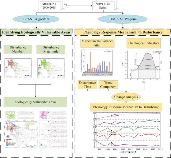
The time series trajectory characteristics of NDVI were extracted by BFAST and TIMESAT. The difference is that BFAST detects the inter-annual variation characteristics of the long-term time series, while TIMESAT detects the local variation characteristics of the NDVI time series (that is, the seasonal changes). The phenological indicators extracted by TIMESAT were divided into 3 categories according to their mean growth phase: start of season (SOS) and end of season (EOS). The maximum during the growth phase is taken as the peak and amplitude, and the integral during the growth phase includes the large integral (the L. integral) and small integral (the S. integral). The S. integral is equal to the L. integral minus the integral of the base line from SOS to EOS. In this study, the SOS and EOS were determined using a fixed threshold approach, with which the smoothed 8-day NDVI reached 25% of the mean amplitude for each growth phase for each pixel. The amplitude was calculated as the peak minus the minimum of the smoothed NDVI values. The minimum of the smoothed NDVI values was set to zero if the smoothed NDVI values were negative. The length of season (LOS) was calculated as the EOS minus SOS. The position of each indicator in the time-series trajectory is shown in Figure 4.

3. Results

3.1. Identification of Ecologically Vulnerable Areas by BFAST

The number and magnitude of abrupt changes in vegetation indicate the instability and sensitivity of the ecosystem, respectively. The number, magnitude, and year of change were detected in the NDVI trend component decomposed using BFAST for each pixel. The spatial distribution and area percentage of the number of changes are shown in Figure 5a,g, respectively. The areas that experienced changes were mainly concentrated in the northwestern part of Jilin Province and accounted for 23.85% of the total area. This indicates that the ecosystem in the northwest is unstable against environmental changes. Using numbers from 1 to 5, as the area percentage decreased, the number increased. The areas with a score of 1 for negative changes were distributed in Siping, Changchun, and Songyuan, accounting for 55.56% of the changed area. Thus, the ecosystems in these areas are relatively stable compared to the areas with numbers greater than 1. The areas with numbers greater than 1 were mainly located in Baicheng city and Songyuan city, as shown in Figure 5d. This suggests that the system stability levels of Baicheng and Songyuan are the worst in the whole region. The larger the magnitude of change, the more sensitive the ecosystem is to external changes. The magnitude of change is shown in Figure 5b,h. The magnitude varied from −2 to 2, within which a magnitude of variation between −0.4 and 0.4 accounted for 86% of the area of change. The percentage of magnitude close to 0 was the highest, which indicates that the ecosystems in most areas are not sensitive to environmental changes. The areas that experienced a negative change, located in Baicheng and Songyuan, occupied 52% of the area of change, which is greater than the areas of positive change, which were located in Siping and Tonghua. This suggests that the areas with the worst anti-disturbance ability in the ecosystem produce a decline in vegetation growth. Figure 5c,i reveal the years of change for the whole region. The whole change span ranged from 2002 to 2016 and was divided into three segments of 2002 to 2004, 2004 to 2008, and 2008 to 2016, according to the characteristics of changes, with increased changes at the beginning followed by decreased changes. The peaks were in 2003, 2005, and 2011. The highest percentage appeared in 2011 (15.4%) in Baicheng and Songyuan. The area of change in 2002 was the lowest (mainly located in Baicheng). The above results show that the ecologically unstable and sensitive areas are located in Baicheng and Songyuan, mostly with one change each, and an abrupt change occurred around 2005 and 2011.
The areas with abrupt declines (negative changes) in vegetation growth after disturbances during the monitoring period were considered to be ecologically vulnerable areas due to their sensitivity and instability. Since the negative changes are mainly concentrated from −0.05 to −0.4, areas with a magnitude of change less than −0.05 and a number of changes greater than 0 were considered ecologically vulnerable areas (Figure 6). Vulnerability was divided into five categories according to the number of changes: low vulnerability, slight vulnerability, moderate vulnerability, high vulnerability, and serious vulnerability, as the number of changes increased, as shown in Table 1.
Figure 6 shows that ecologically vulnerable areas accounted for 13.52% of the total region, mainly concentrated in the northwest (Baicheng, Songyuan) of Jilin Province, where disturbances are caused by drought. The vulnerability of the study area was at a low level, which indicated that resistance against drought disasters was common. Areas of low vulnerability appeared in the southwest of Baicheng and the east of Songyuan, accounting for 46.9% of the vulnerable area; these areas were dominated by cropland and herbaceous. In areas with less precipitation but a large effective irrigation area to reduce the impact of regional drought, wind erosion weakened due to the cropland’s shelterbelts. Areas of slight vulnerability accounted for 37.91% of the vulnerable area and were found in the northwest of Baicheng and to the north of Songyuan, where there was sparse vegetation mixed with cropland and a mosaic of natural vegetation. The precipitation in the region was relatively low, and the irrigation conditions were poor. The landscape was fragmented, the surface structure was simple, and the wind erosion and irrigation conditions were slightly worse in this region than those in areas of low vulnerability. Areas of moderate, high, and serious vulnerability accounted for 15.19% of the vulnerable area and were located in the northeast of Songyuan, which is dominated by sparse vegetation. The wind erosion and soil salinization in this area were the most serious in the entire region. These areas usually suffered from hazardous drought and the most serious vegetation degradation. The poor ecological environment in this area led to vegetation degradation and the poorest ability to cope with drought.

3.2. BFAST Result Verification

A comparison between the NDVI trend and SPEI at the sites is illustrated in Figure 7. In the 5 months of the study (May to September), the NDVI trends corresponded well to the SPEI in terms of their trend and slope. Before April 2007, the drought at the site became serious, leading to a gradual decline in the NDVI trend. The relatively low intensity of the drought (severe drought) period from April to September 2007 (SPEI < −1.5) led to the first drop (abrupt change) of 0.04 in the NDVI trend within a month. After September, 2007, the drought at the site gradually weakened as the SPEI increased, which led to an upward NDVI trend. The second highest intensity drought (extreme drought) period from May 2009, to April 2010 (SPEI < −2) led to a dramatic drop in the NDVI trend. Within two years, the average NDVI value decreased by 0.1. After May 2010, the humidity of the site gradually increased, leading to an upward trend in the NDVI. The decreasing trends were all significant (p < 0.001). In general, the negative changes of NDVI detected by BFAST reflected changes in vegetation after being disturbed.

3.3. Analysis of the Vulnerability of Different Vegetation Types

The vulnerability of different vegetation types against drought was also explored. Figure 8a shows the number of negative changes that represents the instability of each vegetation type. The tree cover, which experienced a negative change of 1, accounted for 99% of the change areas during 2000−2018. Numbers from 1 to 5 were determined for sparse vegetation, while areas with 1 and 2 accounted for 40% and 34%, respectively. The area percentage with a score greater than 1 for other vegetation types was less than that of the sparse vegetation. Tree cover was relatively stable and changed little in response to drought, while sparse vegetation changed frequently and was thus the most unstable in resisting external drought.
The magnitude of change was then compared to determine the sensitivity of different vegetation types. Figure 8b illustrates the mean and the 95% confidence range of the negative magnitude. For the negative changes, sparse vegetation (−0.429) had the lowest mean, while tree cover (−0.092) had the highest mean for the negative magnitude. The 95% confidence range of sparse vegetation was the highest at 0.623, while that of the tree cover was the lowest at 0.175. The results indicated that the order of sensitivity of negative changes from small to large was tree cover, cropland, herbaceous land, shrubland, mosaic natural vegetation, grassland, and sparse vegetation. In general, the strongest and the weakest abilities to resist external drought belonged to tree cover and sparse vegetation, respectively.
Figure 9 shows the percentage of the negative change area for each type of vegetation compared to the total negative change area during 2000−2018. The years with negative changes ranged from 2002 to 2016. The area proportion from large to small was herbaceous land, cropland, mosaic natural vegetation, grassland, shrubland, sparse vegetation, and tree cover. The year with the largest negative change area ranged from 2010 to 2014, which indicates that the northwest area of Jilin suffered more drought during 2010 to 2014 than during the other years.

3.4. Vegetation Phenological Responses to Negative Changes

Finding the pattern underlying the most negative changes for each vegetation type was a prerequisite for exploring the response mechanism of phenology to negative changes. First, the year with the largest proportion was selected according to Figure 9, as shown in Table 2.
Then, the correlation between the NDVI trend representing the growth detected by BFAST and the phenological indicators obtained by TIMESAT were used to screen the phenological indicators related to growth. As shown in Table 3, for the growth phase, the correlation coefficient of SOS was higher than that of EOS in the cropland, mosaic natural vegetation, and grassland. The EOS correlation was higher than that of SOS and length for the herbaceous land, tree cover, shrubland, and sparse vegetation. For all types, the correlation of the peak was higher than that of the amplitude at its maximum. The correlation of the L. integral was higher than that of the S. integral in the integral value. The EOS, SOS, peak, and L. integral were selected as the sensitivity indicators related to growth to explore the phenological responses to negative changes. The peak and L. integral were the indicators for vegetation biomass [53], while the EOS and SOS were indicators of the growth phase.
The trajectory of the NDVI trend component decomposed by BFAST and the sensitive phenological indicators are shown in Figure 10. For the overall change, the NDVI trend was more similar to the L. integral than the peaks for cropland, herbaceous land, shrubland, mosaic natural vegetation, tree cover, and sparse vegetation for the vegetation biomass. For the growth phase, the EOS was consistent with the NDVI trend for all types. The results also demonstrated that the L. integral and EOS were more consistent with growth in the vegetation biomass and the growth phase.
For local changes, the NDVI trend and the sensitive phenological indicators were compared by the years of negative changes. In terms of vegetation biomass, the L. integral decreased due to negative changes of the NDVI trend for cropland, herbaceous land, mosaic natural vegetation, tree cover, shrubland, and grassland, while the L. integral of sparse vegetation increased. Thus, the negative changes had a positive effect on the L. integral for dense vegetation types (Figure 10a–f). For sparse vegetation, the negative change negatively impacted the L. integral. Further, the length of the growth phase was shortened under negative changes for cropland, herbaceous land, tree cover, mosaic natural vegetation, shrubland, and grassland. However, the length for sparse vegetation was extended. For the dense vegetation types, a positive impact on the length of the growth phase was caused by the negative change. For the sparse vegetation, the negative change negatively affected the length.
For the peak changes, both EOS and SOS decreased, while the growth phase advanced. The time of the peak was earlier than that of the previous year, whereas the peak declined for mosaic natural vegetation, shrubland, grassland, and sparse vegetation, as shown in Figure 10c,e–g. For cropland and herbaceous land, EOS and SOS both increased, and the growth phase was delayed. The time of the peak was late, and an increase in the peak is shown in Figure 10a,b. When the decrease in EOS was greater than the increase in SOS, the growth phase had advanced. When the year of the peak was earlier, the peak declined for tree cover, as shown in Figure 10d. In summary, for all vegetation types, the variation of the peak depended on the peak time. Specifically, the peak time was earlier when the peak declined. Otherwise, the time of the peak was delayed as the peak rose.

4. Discussion

4.1. Spatial Distribution of the Ecologically Vulnerable Area

The results in Section 3.1 show that the ecologically vulnerable areas were located in the northwest area of Jilin Province. Compared with the southeastern part, which is covered by trees, the northwestern part was mainly covered by cropland and sparse vegetation, where more frequent and severe drought occurred. This result is consistent with the fact that the stability of the trees was greater than the stability of sparse vegetation and cropland, as shown in Section 3.3. Moreover, the results of this paper are consistent with previous research [54]. Consequently, the method based on abrupt change detection from RS time-series data is able to identify ecologically vulnerable areas. Thus, the regional disaster prevention capabilities were identified effectively by BFAST. The northwest area contained arid and semi-arid areas and the vulnerable ecological zone of cropland and grass in northeastern China. This study area belongs to the junction between a temperate continental climate and a temperate monsoon climate, which is the reason for the complex community structure, high degree of environmental heterogeneity due to poor anti-interference abilities, and climatic sensitivity of the ecological system, as well as the space–time fluctuations with a high frequency and weak edge effect in the area. In the agricultural belt of the northwest, as a result of long-term continuous cropping and the excessive application of pesticides and fertilizers, soil fertility has declined. The degradation and erosion of black soil have become gradually more serious under the impact of non-point-source pollution and wind erosion. The surface temperature and biological distribution structure have also been changed by human interference. However, soil salinization and grassland degradation have reduced drought resistance in the northern region, which is located in the agricultural and pastoral ecotone zone. At the same time, blind reclamation, wetland environment deterioration, function decline, and the extent of vulnerable ecosystems were much worse.

4.2. The Response of Vegetation Phenology to Negative Changes

As shown in Figure 10, parts of the NDVI trends were not similar to the phenology indicators. For example, the changes of the phenological indicators in the cropland from 2005 to 2006 were more significant than those from 2011 to 2012. The environment changed from humid to drought in 2005–2006, as shown in Figure 7. Although the degree of drought did not reach an extreme level, the water needed for vegetation growth changed from a sufficient deficit, and vegetation growth began to be stressed. There were also some fluctuations in the phenological indicators. Compared to the changes in 2007–2010, the changes in the phenological trajectory during 2005–2006 were relatively short-lived and had less of an impact on the overall trend. The phenological changes caused by the severe drought in 2007–2010 had a greater impact on the trend changes in the following years and was a turning point that affected the changes in phenological trends.
In this paper, the relative amount of vegetation biomass and length of the growing period were decreased by negative changes. However, the peak and SOS were less affected by negative changes. This indicates that the impact of negative change on vegetation phenology has long-term effects. When vegetation growth suddenly drops, the balanced state of the interactive process between vegetation and the environment is broken. Therefore, vegetation constantly adjusts itself to adapt to the changing environment. For example, vegetation closes its stomata to reduce water loss and fit the drought status. Vegetation needs a period of recovery before reaching its next stable period. Therefore, negative changes had a more significant effect on the cumulative values than the instantaneous values. Additionally, when a negative change occurred after the time of peak, the effect of the negative change was also independent of the peak. The peak declined as the peak time advanced, while the peak rose as the peak time was delayed. Advancement of the peak time indicated that the vegetation was not located in the correct ecological environment and was much susceptible to the stress of water and nutrients. Thus, the peak declined. Otherwise, when the peak time was delayed, there was enough available soil water, heat, and fertilizer to improve photosynthesis efficiency. Consequently, the peak rose. In general, the results of this study show that when the changes in phenology are known, changes in the surrounding environment can be inferred. When the length of the growing period and the relative amount of vegetation biomass decreased significantly, vegetation growth was under environmental stress, indicating that the environment could gradually deteriorate.

4.3. Limitations and Future Work

In this paper, the negative changes of NDVI were used to identify the ecologically vulnerable areas under drought, although this method is also applicable to other disturbances that cause declines in vegetation growth, such as insect infestations and flood disasters, because the negative changes in the NDVI reflect the sensitivity and stability of vegetation being disturbed. However, specific disturbances need to be compared with the results of BFAST to verify that the vegetation change is, in fact, caused by the disturbance.
Three major limitations of this study should be discussed further. First, vulnerable areas were identified based only on negative changes in vegetation growth. This limitation led to overlooking areas of low vegetation cover. So, areas with less than 10% vegetation cover were excluded in the vulnerable area analysis. This was a necessary trade-off because it is difficult to assess ecological vulnerability in areas of low vegetation cover. This, however, should not be a great concern as only a small proportion of the study area (1.54%) was characterized by low vegetation cover. Second, in this paper, the relationship of change between phenology and negative changes was revealed. However, the sensitivity between negative changes and phenological changes could be further explored, such as the range of negative changes that will not trigger changes in phenology and the threshold of negative changes that will affect changes in phenology. Third, when comparing the negative changes for different vegetation types, this paper assumed that the soil profile and depth were homogeneous. The influences of different soil depths and slopes on the drought resistance of vegetation will be considered in future work. Further investigations on this issue should thus be carried out in the future.

5. Conclusions

On the basis of the changes in vegetation growth in Jilin Province, China, during 2000–2018, a method to identify ecologically vulnerable areas was developed based on detecting abrupt changes in NDVI time series. Then, the response of phenology to negative changes was explored by analyzing the phenological indictors and the NDVI trend. The following conclusions were reached:
(1)
In this paper, an ecologically fragile zone identification framework based on the breakpoint detection of the BFAST NDVI time series was proposed. By identifying ecologically vulnerable areas to detect the number of negative changes and the magnitude of negative changes in vegetation growth over many years, we fully considered the long-term stability of vegetation growth and sensitivity to specific disturbances. This method can accurately reflect the long-term and short-term changes in vegetation growth and has better applicability in semi-arid regions.
(2)
During the past 19 years, northwest Jilin Province located in the semi-arid area was identified as ecologically vulnerable, primarily with low and slight vulnerability, where rainfall is scarce. Moreover, artificial irrigation cannot meet the needs of vegetation growth. Moisture is the main limiting factor leading to the vulnerability of the region’s ecological environment.
(3)
Compared to other vegetation types with dense coverage, 60% of the area had a number of negative changes greater than 1, a much larger area than that of other vegetation types (less than 50%). The magnitude of change in sparse vegetation was −0.429, which is the lowest among the vegetation types. This shows that sparse vegetation is more susceptible to drought. Therefore, increasing the vegetation coverage or changing to more stable vegetation types can reduce the fragility in ecologically vulnerable areas.
(4)
For vegetation types with dense coverage, the impact of negative changes on vegetation phenology shows long-term effects. The negative changes in the NDVI trends of various types of vegetation led to a fluctuation range of the integral value from −0.06 to −6.9 and a phenological period length from −0.3 to −5.4; the peak value varied from −0.11 to 0.12. Negative change had a significant effect on the cumulative values of the growth phase, such as the relative amount of vegetation biomass and the length of the growing period, but less of an effect on the instantaneous value of the peak. Detecting changes in the growth phase or the integral value could be used to predict whether the vegetation growth experiences a negative change.

Author Contributions

Conceptualization, J.M. and W.Y.; data curation, W.C. and L.G.; investigation, W.C.; methodology, J.M., C.Z., and W.Y.; project administration, J.M.; software, H.W.; supervision, C.Z.; validation, J.M. and W.C.; visualization, L.G.; writing—original draft, J.M.; writing—review and editing, C.Z. and H.G. All authors approved the version submitted for publication. All authors have read and agreed to the published version of the manuscript.

Funding

This research was supported by the National Key Research and Development Program of China (project No. 2018YFE0122700).

Acknowledgments

The authors are grateful for research assistance from Dehai Zhu, Yongxia Yang, Jianyu Yang, Dongling Zhao, Xiaochuang Yao, Jinyou Li, Changzhi Wang, Zhengyu Liu, and Yuan Yao. The insightful and constructive comments of the anonymous reviewers are also appreciated.

Conflicts of Interest

The authors declare no conflict of interest.

References

  1. Feehan, J.; Harley, M.; Minnen, J. Climate change in Europe. Impact on terrestrial ecosystems and biodiversity. A review. Agron. Sustain. Dev. 2009, 29, 409–421. [Google Scholar] [CrossRef]
  2. Shriver, R.K.; Andrews, C.M.; Arkle, R.S.; Barnard, D.M.; Duniway, M.C.; Germino, M.J.; Pilliod, D.S.; Pyke, D.A.; Welty, J.L.; Bradford, J.B. Transient population dynamics impede restoration and may promote ecosystem transformation after disturbance. Ecol. Lett. 2019, 22, 1357–1366. [Google Scholar] [CrossRef] [PubMed]
  3. E Fernández-Giménez, M.; Allington, G.; Angerer, J.; Reid, R.S.; Jamsranjav, C.; Ulambayar, T.; Hondula, K.; Baival, B.; Batbuyan, B.; Altanzul, T.; et al. Using an integrated social-ecological analysis to detect effects of household herding practices on indicators of rangeland resilience in Mongolia. Environ. Res. Lett. 2018, 13, 075010. [Google Scholar] [CrossRef]
  4. Reid, R.S.; Fernández-Giménez, M.E.; Galvin, K.A. Dynamics and Resilience of Rangelands and Pastoral Peoples Around the Globe. Annu. Rev. Environ. Resour. 2014, 39, 217–242. [Google Scholar] [CrossRef]
  5. Turner, B.L.; Kasperson, R.E.; Matson, P.A.; McCarthy, J.J.; Corell, R.W.; Christensen, L.; Eckley, N.; Kasperson, J.X.; Luers, A.; Martello, M.L.; et al. A framework for vulnerability analysis in sustainability science. Proc. Natl. Acad Sci. USA 2003, 100, 8074–8079. [Google Scholar] [CrossRef] [Green Version]
  6. Hong, W.; Jiang, R.; Yang, C.; Zhang, F.; Su, M.; Liao, Q. Establishing an ecological vulnerability assessment indicator system for spatial recognition and management of ecologically vulnerable areas in highly urbanized regions: A case study of Shenzhen, China. Ecol. Indic. 2016, 69, 540–547. [Google Scholar] [CrossRef]
  7. Zhumanova, M.; Mönnig, C.; Hergarten, C.; Darr, D.; Wrage-Mönnig, N. Assessment of vegetation degradation in mountainous pastures of the Western Tien-Shan, Kyrgyzstan, using eMODIS NDVI. Ecol. Indic. 2018, 95, 527–543. [Google Scholar] [CrossRef]
  8. Chen, X.; Wang, W.; Chen, J.; Zhu, X.; Shen, M.; Gan, L.; Cao, X. Does any phenological event defined by remote sensing deserve particular attention? An examination of spring phenology of winter wheat in Northern China. Ecol. Indic. 2020, 116, 106456. [Google Scholar] [CrossRef]
  9. Yuan, F. Land-cover change and environmental impact analysis in the Greater Mankato area of Minnesota using remote sensing and GIS modelling. Int. J. Remote. Sens. 2007, 29, 1169–1184. [Google Scholar] [CrossRef]
  10. Fraga, H.; Amraoui, M.; Malheiro, A.C.; Moutinho-Pereira, J.; Eiras-Dias, J.; Silvestre, J.; Santos, J.A. Examining the relationship between the Enhanced Vegetation Index and grapevine phenology. Eur. J. Remote. Sens. 2014, 47, 753–771. [Google Scholar] [CrossRef]
  11. Pei, H.; Fang, S.; Lin, L.; Qin, Z.; Wang, X. Methods and applications for ecological vulnerability evaluation in a hyper-arid oasis: A case study of the Turpan Oasis, China. Environ. Earth Sci. 2015, 74, 1449–1461. [Google Scholar] [CrossRef] [Green Version]
  12. Lewontin, R.C. The meaning of stability. In Brookhaven Symposia in Biology; Brookhaven National Laboratory: Upton, NY, USA, 1969; Volume 22, pp. 13–24. [Google Scholar]
  13. Romer, H.; Willroth, P.; Kaiser, G.; Vafeidis, A.T.; Ludwig, R.; Sterr, H.; Diez, J.R. Potential of remote sensing techniques for tsunami hazard and vulnerability analysis – a case study from Phang-Nga province, Thailand. Nat. Hazards Earth Syst. Sci. 2012, 12, 2103–2126. [Google Scholar] [CrossRef] [Green Version]
  14. Smith, A.M.S.; Kolden, C.A.; Tinkham, W.T.; Talhelm, A.F.; Marshall, J.D.; Hudak, A.T.; Boschetti, L.; Falkowski, M.J.; Greenberg, J.A.; Anderson, J.W.; et al. Remote sensing the vulnerability of vegetation in natural terrestrial ecosystems. Remote. Sens. Environ. 2014, 154, 322–337. [Google Scholar] [CrossRef]
  15. Ratajczak, Z.; Carpenter, S.R.; Ives, A.R.; Kucharik, C.J.; Ramiadantsoa, T.; Stegner, M.A.; Williams, J.W.; Zhang, J.; Turner, M.G. Abrupt Change in Ecological Systems: Inference and Diagnosis. Trends Ecol. Evol. 2018, 33, 513–526. [Google Scholar] [CrossRef]
  16. Bulletin of the People’s Republic of China Home Page. Available online: http://www.gov.cn/gongbao/content/2009/content_1250928.htm (accessed on 14 October 2020).
  17. Jiang, L.; Huang, X.; Wang, F.; Liu, Y.; An, P. Method for evaluating ecological vulnerability under climate change based on remote sensing: A case study. Ecol. Indic. 2018, 85, 479–486. [Google Scholar] [CrossRef]
  18. Richardson, A.D.; Keenan, T.F.; Migliavacca, M.; Ryu, Y.; Sonnentag, O.; Toomey, M. Climate change, phenology, and phenological control of vegetation feedbacks to the climate system. Agric. For. Meteorol. 2013, 169, 156–173. [Google Scholar] [CrossRef]
  19. Sankey, J.B.; Wallace, C.S.; Ravi, S. Phenology-based, remote sensing of post-burn disturbance windows in rangelands. Ecol. Indic. 2013, 30, 35–44. [Google Scholar] [CrossRef]
  20. Ma, X.; Huete, A.; Moran, S.; Ponce-Campos, G.; Eamus, D. Abrupt shifts in phenology and vegetation productivity under climate extremes. J. Geophys. Res. Biogeosciences 2015, 120, 2036–2052. [Google Scholar] [CrossRef]
  21. Minin, A.A.; Trofimov, I.E.; Zakharov, V.M. Assessment of the Stability of Phenological Indices of the Silver Birch Betula pendula under Climate Change. Biol. Bull. 2020, 47, 149–152. [Google Scholar] [CrossRef]
  22. Verbesselt, J.; Zeileis, A.; Herold, M. Near real-time disturbance detection using satellite image time series. Remote. Sens. Environ. 2012, 123, 98–108. [Google Scholar] [CrossRef]
  23. Jones, M.O.; Kimball, J.S.; Jones, L.A. Satellite microwave detection of boreal forest recovery from the extreme 2004 wildfires in Alaska and Canada. Glob. Chang. Biol. 2013, 19, 3111–3122. [Google Scholar] [CrossRef] [PubMed]
  24. Bullock, E.L.; Woodcock, C.E.; Olofsson, P. Monitoring tropical forest degradation using spectral unmixing and Landsat time series analysis. Remote. Sens. Environ. 2020, 238, 110968. [Google Scholar] [CrossRef]
  25. Wen, L.; Saintilan, N. Climate phase drives canopy condition in a large semi-arid floodplain forest. J. Environ. Manag. 2015, 159, 279–287. [Google Scholar] [CrossRef] [PubMed]
  26. Qu, C.; Hao, X.; Qu, J.J. Monitoring Extreme Agricultural Drought over the Horn of Africa (HOA) Using Remote Sensing Measurements. Remote. Sens. 2019, 11, 902. [Google Scholar] [CrossRef] [Green Version]
  27. Price, B.; Waser, L.T.; Wang, Z.; Marty, M.; Ginzler, C.; Zellweger, F. Predicting biomass dynamics at the national extent from digital aerial photogrammetry. Int. J. Appl. Earth Obs. Geoinformation 2020, 90, 102116. [Google Scholar] [CrossRef]
  28. DeChant, B.; Ryu, Y.; Badgley, G.; Zeng, Y.; Berry, J.A.; Zhang, Y.; Goulas, Y.; Li, Z.; Zhang, Q.; Kang, M.; et al. Canopy structure explains the relationship between photosynthesis and sun-induced chlorophyll fluorescence in crops. Remote. Sens. Environ. 2020, 241, 111733. [Google Scholar] [CrossRef] [Green Version]
  29. Malenovský, Z.; Mishra, K.B.; Zemek, F.; Rascher, U.; Nedbal, L. Scientific and technical challenges in remote sensing of plant canopy reflectance and fluorescence. J. Exp. Bot. 2009, 60, 2987–3004. [Google Scholar] [CrossRef] [PubMed] [Green Version]
  30. Ju, J.; Masek, J.G. The vegetation greenness trend in Canada and US Alaska from 1984–2012 Landsat data. Remote. Sens. Environ. 2016, 176, 1–16. [Google Scholar] [CrossRef]
  31. Qian, Y.; Yang, Z.; Di, L.; Rahman, S.; Tan, Z.; Xue, L.; Gao, F.; Yu, E.; Zhang, X. Crop Growth Condition Assessment at County Scale Based on Heat-Aligned Growth Stages. Remote. Sens. 2019, 11, 2439. [Google Scholar] [CrossRef] [Green Version]
  32. Zhou, Z.; Ding, Y.; Shi, H.; Cai, H.; Fu, Q.; Liu, S.; Li, T. Analysis and prediction of vegetation dynamic changes in China: Past, present and future. Ecol. Indic. 2020, 117, 106642. [Google Scholar] [CrossRef]
  33. Watts, L.M.; Laffan, S.W. Effectiveness of the BFAST algorithm for detecting vegetation response patterns in a semi-arid region. Remote. Sens. Environ. 2014, 154, 234–245. [Google Scholar] [CrossRef]
  34. Chen, H.; Liang, Q.; Liang, Z.; Liu, Y.; Xie, S. Remote-sensing disturbance detection index to identify spatio-temporal varying flood impact on crop production. Agric. For. Meteorol. 2019, 180–191. [Google Scholar] [CrossRef]
  35. White, P.S.; Pickett, S.T.A. Chapter 1—Natural Disturbance and Patch Dynamics: An Introduction. In The Ecology of Natural Disturbance and Patch Dynamics; Pickett, S.T.A., White, P.S., Eds.; Academic Press: San Diego, CA, USA, 1985; pp. 3–13. [Google Scholar] [CrossRef]
  36. Yang, Y.; Erskine, P.D.; Lechner, A.M.; Mulligan, D.; Zhang, S.; Wang, Z. Detecting the dynamics of vegetation disturbance and recovery in surface mining area via Landsat imagery and LandTrendr algorithm. J. Clean. Prod. 2018, 178, 353–362. [Google Scholar] [CrossRef]
  37. Morrison, J.; Higginbottom, T.P.; Symeonakis, E.; Jones, M.J.; Omengo, F.; Walker, S.L.; Cain, B. Detecting Vegetation Change in Response to Confining Elephants in Forests Using MODIS Time-Series and BFAST. Remote. Sens. 2018, 10, 1075. [Google Scholar] [CrossRef] [Green Version]
  38. Li, M.; Huang, C.; Zhu, Z.; Wen, W.; Xu, D.; Liu, A. Use of remote sensing coupled with a vegetation change tracker model to assess rates of forest change and fragmentation in Mississippi, USA. Int. J. Remote. Sens. 2009, 30, 6559–6574. [Google Scholar] [CrossRef]
  39. Shen, X.-J.; An, R.; Feng, L.; Ye, N.; Zhu, L.; Li, M. Vegetation changes in the Three-River Headwaters Region of the Tibetan Plateau of China. Ecol. Indic. 2018, 93, 804–812. [Google Scholar] [CrossRef]
  40. Verbesselt, J.; Hyndman, R.; Newnham, G.; Culvenor, D. Detecting trend and seasonal changes in satellite image time series. Remote. Sens. Environ. 2010, 114, 106–115. [Google Scholar] [CrossRef]
  41. Fang, X.; Zhu, Q.; Ren, L.; Chen, H.; Wang, K.; Peng, C. Large-scale detection of vegetation dynamics and their potential drivers using MODIS images and BFAST: A case study in Quebec, Canada. Remote. Sens. Environ. 2018, 206, 391–402. [Google Scholar] [CrossRef]
  42. Schultz, M.; Clevers, J.G.; Carter, S.; Verbesselt, J.; Avitabile, V.; Quang, H.V.; Herold, M. Performance of vegetation indices from Landsat time series in deforestation monitoring. Int. J. Appl. Earth Obs. Geoinformation 2016, 52, 318–327. [Google Scholar] [CrossRef]
  43. Roerink, G.J.; Menenti, M.; Verhoef, W. Reconstructing cloudfree NDVI composites using Fourier analysis of time series. Int. J. Remote. Sens. 2000, 21, 1911–1917. [Google Scholar] [CrossRef]
  44. Colditz, R.R.; Conrad, C.; Wehrmann, T.; Schmidt, M.; Dech, S. TiSeG: A Flexible Software Tool for Time-Series Generation of MODIS Data Utilizing the Quality Assessment Science Data Set. IEEE Trans. Geosci. Remote. Sens. 2008, 46, 3296–3308. [Google Scholar] [CrossRef]
  45. McKellip, R.; Prados, D.; Ryan, R.; Ross, K.; Spruce, J.; Gasser, G.; Greer, R. Remote-Sensing Time Series Analysis, a Vegetation Monitoring Tool. Front. Environ. Sci. 2008. [Google Scholar] [CrossRef] [Green Version]
  46. Jönsson, P.; Eklundh, L. TIMESAT—a program for analyzing time-series of satellite sensor data. Comput. Geosci. 2004, 30, 833–845. [Google Scholar] [CrossRef] [Green Version]
  47. Stanimirova, R.; Cai, Z.; Melaas, E.; Gray, J.M.; Eklundh, L.; Jönsson, P.; Friedl, M.A. Gray An Empirical Assessment of the MODIS Land Cover Dynamics and TIMESAT Land Surface Phenology Algorithms. Remote. Sens. 2019, 11, 2201. [Google Scholar] [CrossRef] [Green Version]
  48. Wang, Q.; Wu, J.; Li, X.; Zhou, H.; Yang, J.; Geng, G.; An, X.; Liu, L.; Tang, Z. A comprehensively quantitative method of evaluating the impact of drought on crop yield using daily multi-scale SPEI and crop growth process model. Int. J. Biometeorol. 2016, 61, 685–699. [Google Scholar] [CrossRef] [PubMed]
  49. Vicente-Serrano, S.M.; Beguería, S.; López-Moreno, J.I. A Multiscalar Drought Index Sensitive to Global Warming: The Standardized Precipitation Evapotranspiration Index. J. Clim. 2010, 23, 1696–1718. [Google Scholar] [CrossRef] [Green Version]
  50. Pérez-Hoyos, A.; Rembold, F.; Kerdiles, H.; Gallego, J. Comparison of Global Land Cover Datasets for Cropland Monitoring. Remote. Sens. 2017, 9, 1118. [Google Scholar] [CrossRef] [Green Version]
  51. Jönsson, P.; Eklundh, L. Seasonality extraction by function fitting to time-series of satellite sensor data. IEEE Trans. Geosci. Remote. Sens. 2002, 40, 1824–1832. [Google Scholar] [CrossRef]
  52. Walker, J.J.; Soulard, C.E. Phenology Patterns Indicate Recovery Trajectories of Ponderosa Pine Forests After High-Severity Fires. Remote. Sens. 2019, 11, 2782. [Google Scholar] [CrossRef] [Green Version]
  53. Tian, F.; Brandt, M.; Liu, Y.Y.; Verger, A.; Tagesson, T.; Diouf, A.A.; Rasmussen, K.; Mbow, C.; Wang, Y.; Fensholt, R. Remote sensing of vegetation dynamics in drylands: Evaluating vegetation optical depth (VOD) using AVHRR NDVI and in situ green biomass data over West African Sahel. Remote. Sens. Environ. 2016, 177, 265–276. [Google Scholar] [CrossRef] [Green Version]
  54. Guo, Y.; Wang, R.; Tong, Z.; Liu, X.; Zhang, J. Dynamic Evaluation and Regionalization of Maize Drought Vulnerability in the Midwest of Jilin Province. Sustainability 2019, 11, 4234. [Google Scholar] [CrossRef] [Green Version]
Figure 1. (a) Spatial distribution of land cover types in 2015 in Jilin Province (data from ESA CCI-LC); (b) the spatial distribution of elevation in Jilin Province (DEM from GDEMDEM data with a 30-m spatial resolution).
Remotesensing 12 03371 g001
Figure 2. Flowchart of the identification of ecologically vulnerable areas and exploration of the phenological response mechanism for disturbances using Breaks for Additive Season and Trend (BFAST) and TIMESAT from the remote sensing (RS) time series.
Remotesensing 12 03371 g002
Figure 3. BFAST detected that one breakpoint and a negative magnitude occurred in 2008 in the time-series normalized difference vegetation index (NDVI) during 2000–2018.
Remotesensing 12 03371 g003
Figure 4. Phenological indicators extracted from TIMESAT: amplitude, start of season (SOS), end of season (EOS), base value, large integral (L. integral), small integral (S. integral), peak, and growth phase length (length).
Remotesensing 12 03371 g004
Figure 5. Abrupt change of the NDVI time series in Jilin Province during 2000–2018: (a) spatial distribution of the number of changes; (b) spatial distribution of the magnitude of change; (c) spatial distribution of the year of change; (df) spatial disturbance of the number, magnitude, and year in Baicheng and Songyuan, respectively; (g) area percentage of the number of changes; (h) area percentage of the magnitude of change; (i) area percentage of the year of change.
Remotesensing 12 03371 g005
Figure 6. Spatial distribution of the ecologically vulnerable area and the BFAST results for different levels of vulnerability: (ae) Spatial distribution and temporal changes of low vulnerability, slight vulnerability, moderate vulnerability, high vulnerability, and serious vulnerability, respectively.
Remotesensing 12 03371 g006
Figure 7. The 5-month (May–September) standardized precipitation evapotranspiration index (SPEI) (orange bar) and NDVI trend (line) components decomposed by BFAST at Qianan station. C, D, E, F, respectively, represent the NDVI trend for 4 pixels near the site extracted by BFAST.
Remotesensing 12 03371 g007
Figure 8. (a) Area percentage of the number of negative changes in different vegetation types between 2000 and 2018. (b) Interval plot of the negative magnitude for different vegetation types (the blue line indicates the range of the 95% confidence intervals, and the red dot in the center is the mean value).
Remotesensing 12 03371 g008
Figure 9. Area percentages of negative changes in each vegetation area during 2000–2018.
Remotesensing 12 03371 g009
Figure 10. The trajectory changes of the trend component and the sensitive phenological indicators extracted by TIMESAT. (a) trajectory changes of cropland, (b) trajectory changes of herbaceous, (c) trajectory changes of mosaic natural vegetation, (d) trajectory changes of tree cover, (e) trajectory changes of shrubland, (f) trajectory changes of grassland, and (g) trajectory changes of sparse vegetation.
Remotesensing 12 03371 g010aRemotesensing 12 03371 g010b
Table 1. Vulnerability level classification standard.
Number of Negative ChangesVulnerability
1Low Vulnerability
2Slight Vulnerability
3Moderate Vulnerability
4High Vulnerability
5Serious Vulnerability
Table 2. Statistics of the negative changes with the largest areas for each vegetation type.
Vegetation TypesNumber of ChangesYear of Change
Cropland12011
Herbaceous12012
Mosaic Natural Vegetation12012
Tree Cover12009
Shrubland12014
Grassland12010
Sparse Vegetation12011
Table 3. The correlation coefficients of phenological indicators and the NDVI trend for vegetation types.
Vegetation TypesGrowth PhaseMaximum Integral
SOSEOSAmplitudePeakL. integralS. integral
Cropland−0.730.160.610.830.890.74
Herbaceous−0.430.54−0.150.180.750.68
Mosaic Natural Vegetation0.680.650.760.860.950.83
Tree Cover−0.270.460.420.780.790.57
Shrubland−0.50.580.710.740.880.74
Grassland−0.28−0.270.690.920.810.70
Sparse Vegetation0.290.710.150.650.670.46
Publisher’s Note: MDPI stays neutral with regard to jurisdictional claims in published maps and institutional affiliations.

