Moving Target Imaging Using GNSS-Based Passive Bistatic Synthetic Aperture Radar


Abstract
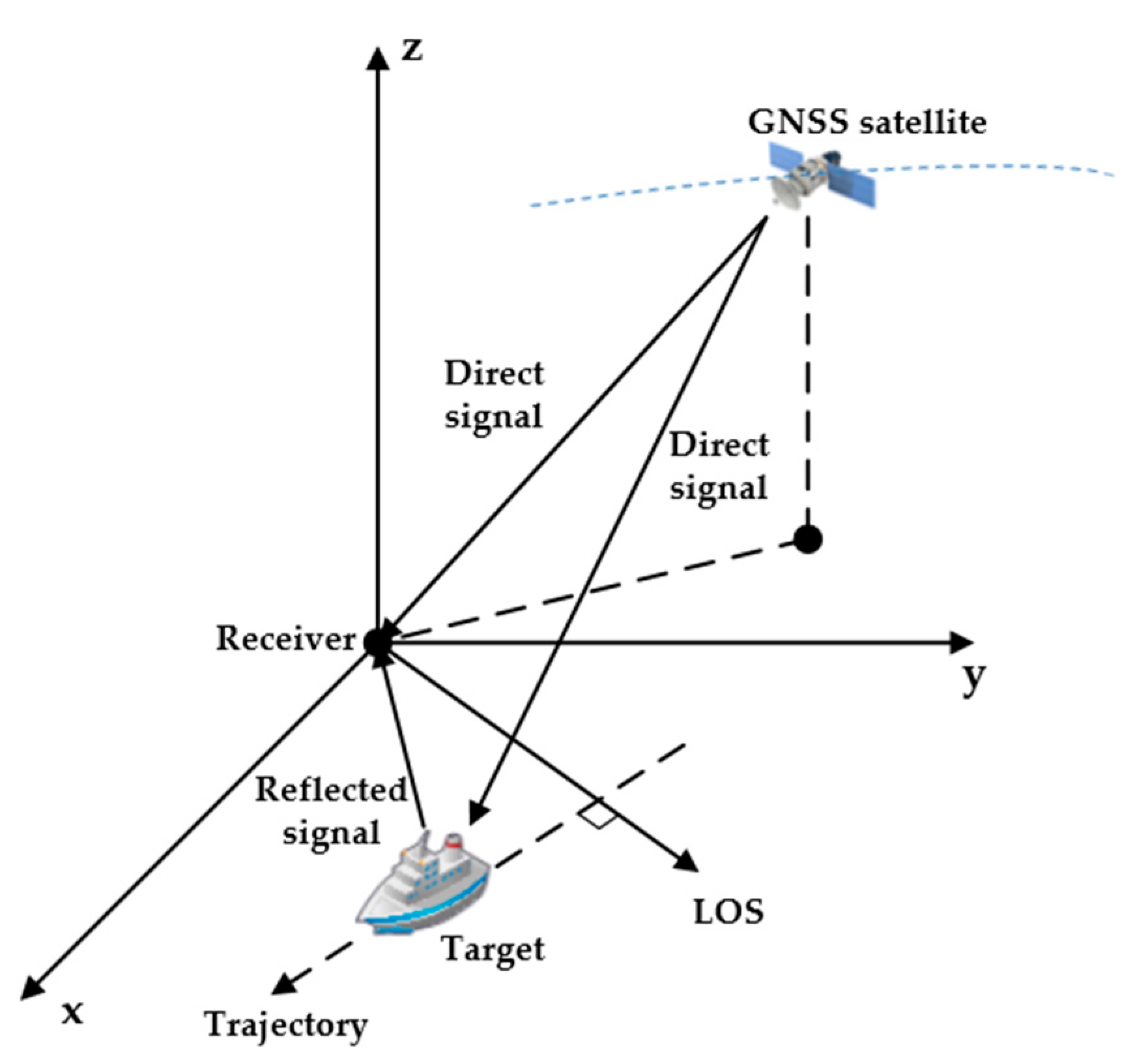
:1. Introduction
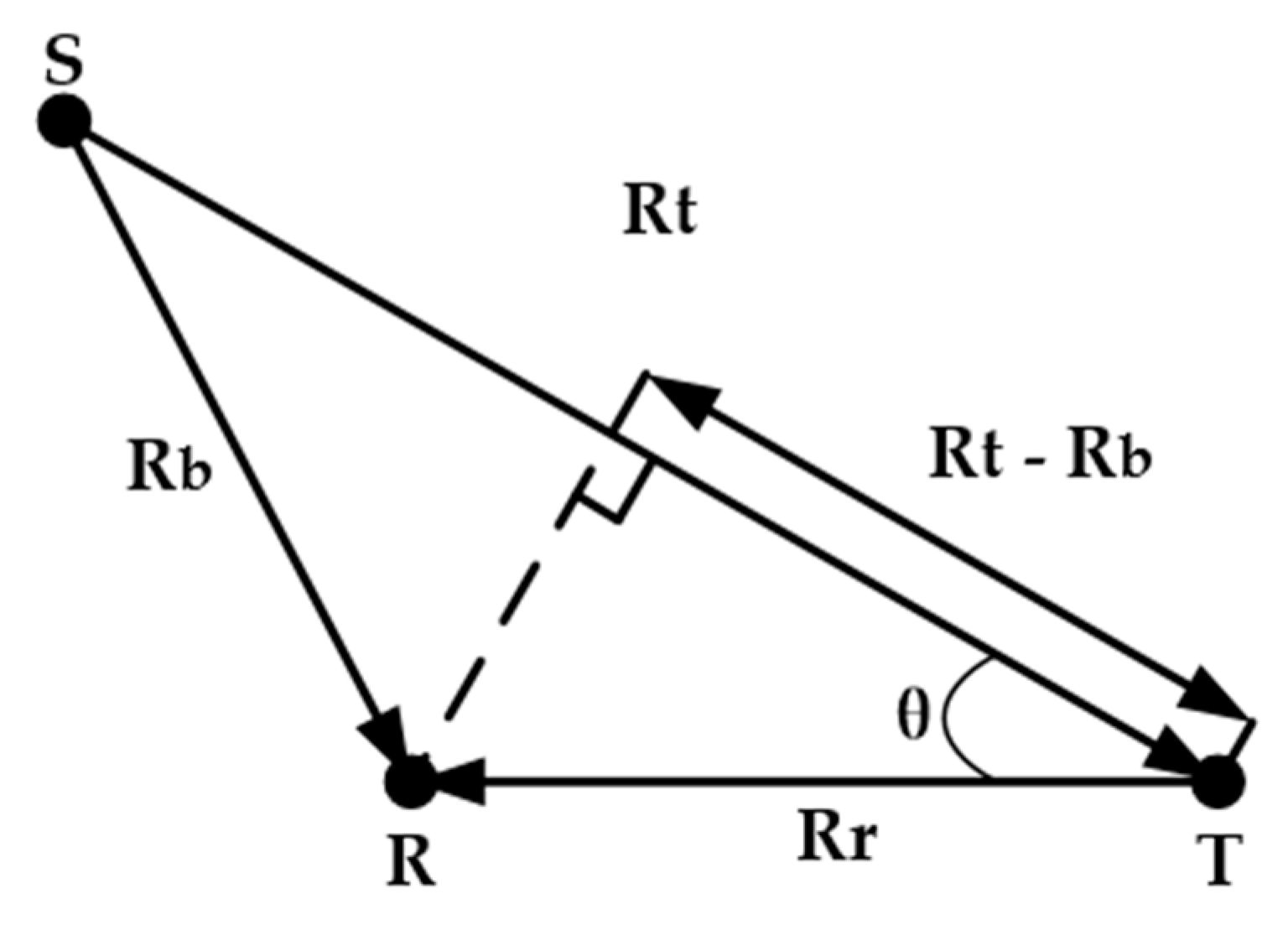
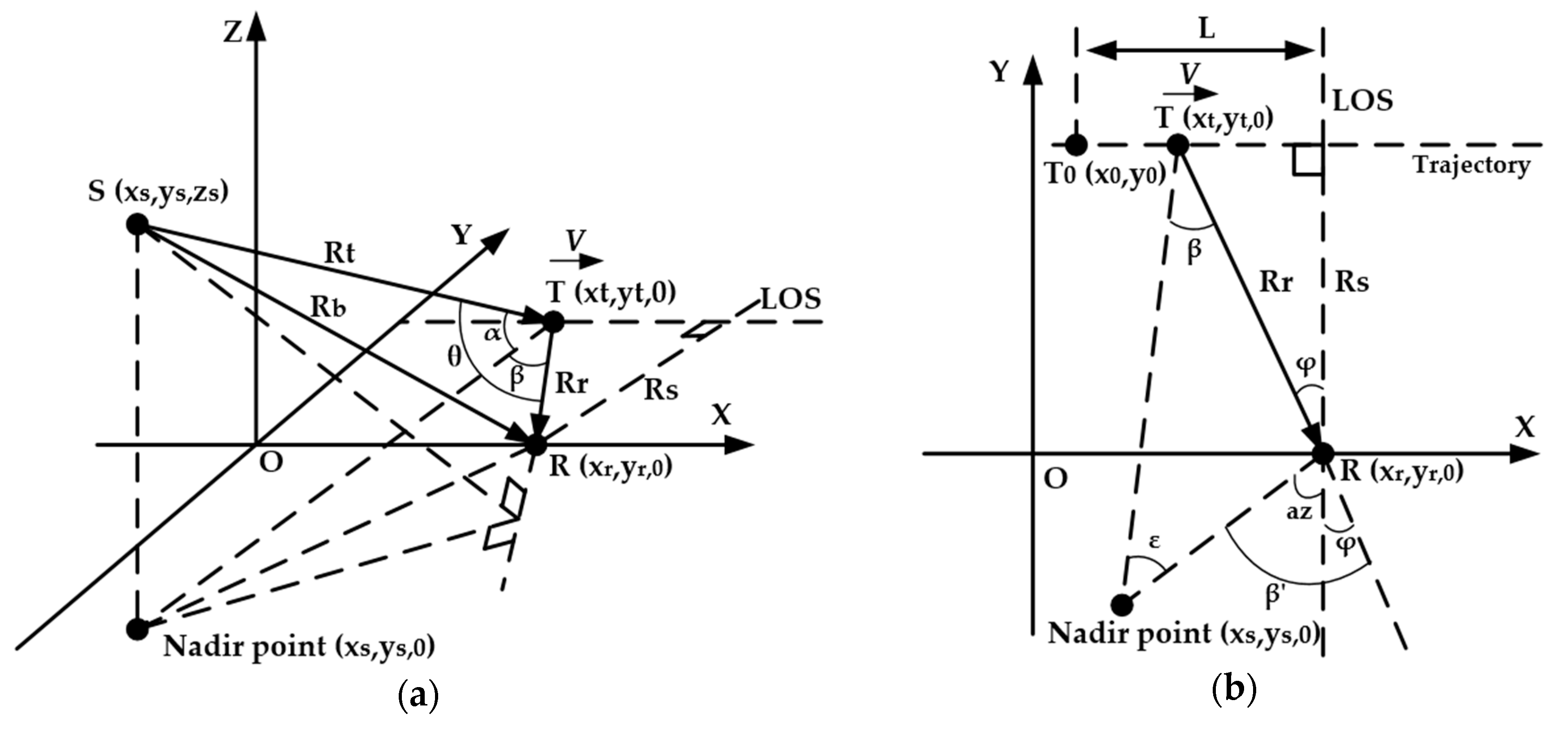
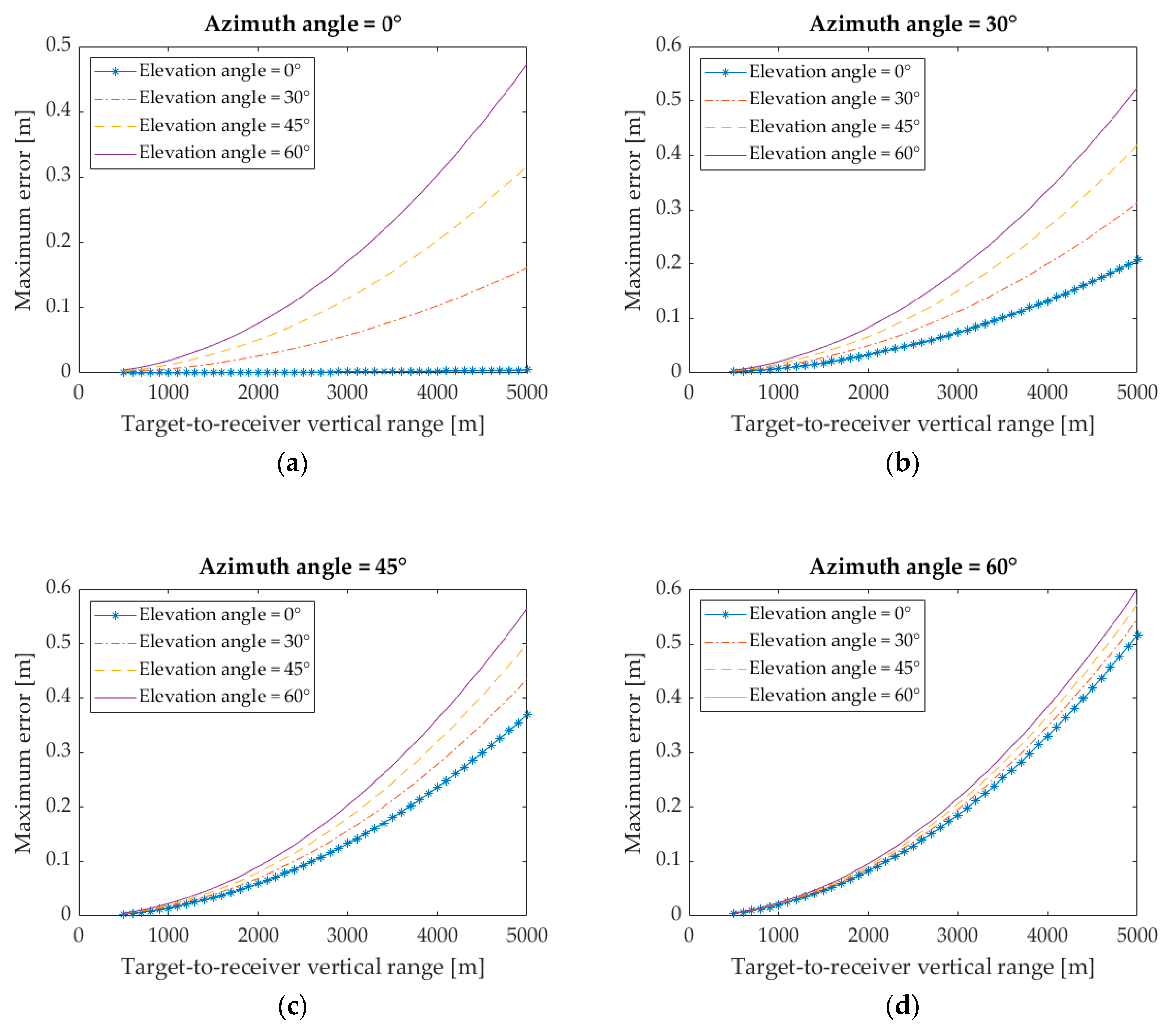
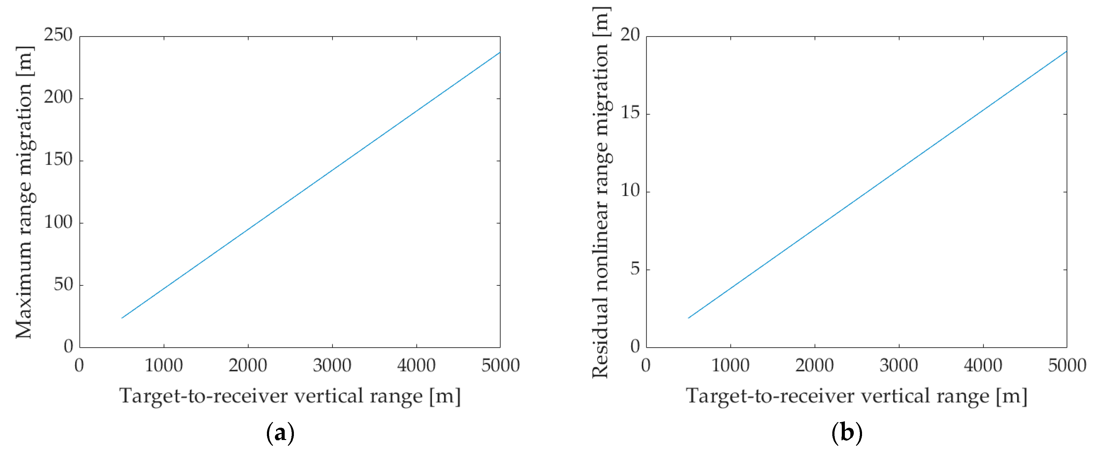
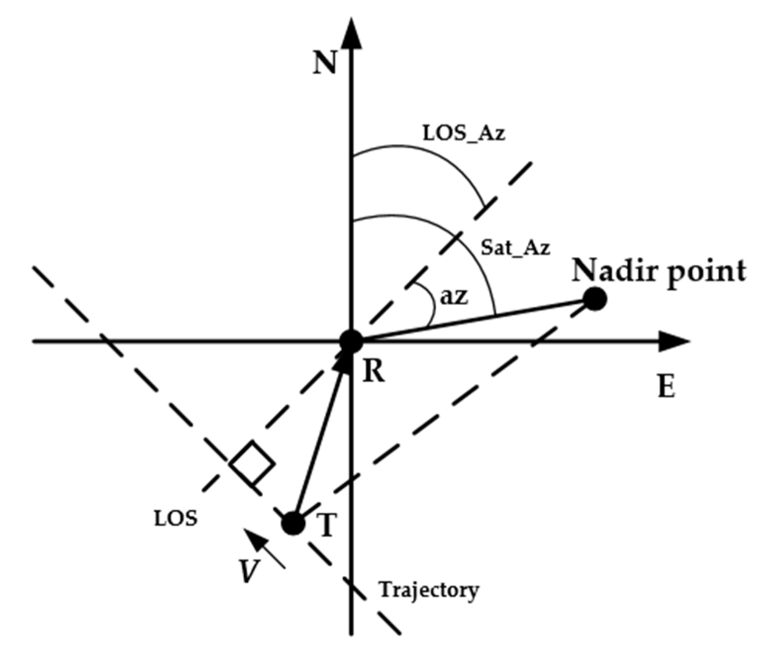
2. Approximate Bistatic Range History
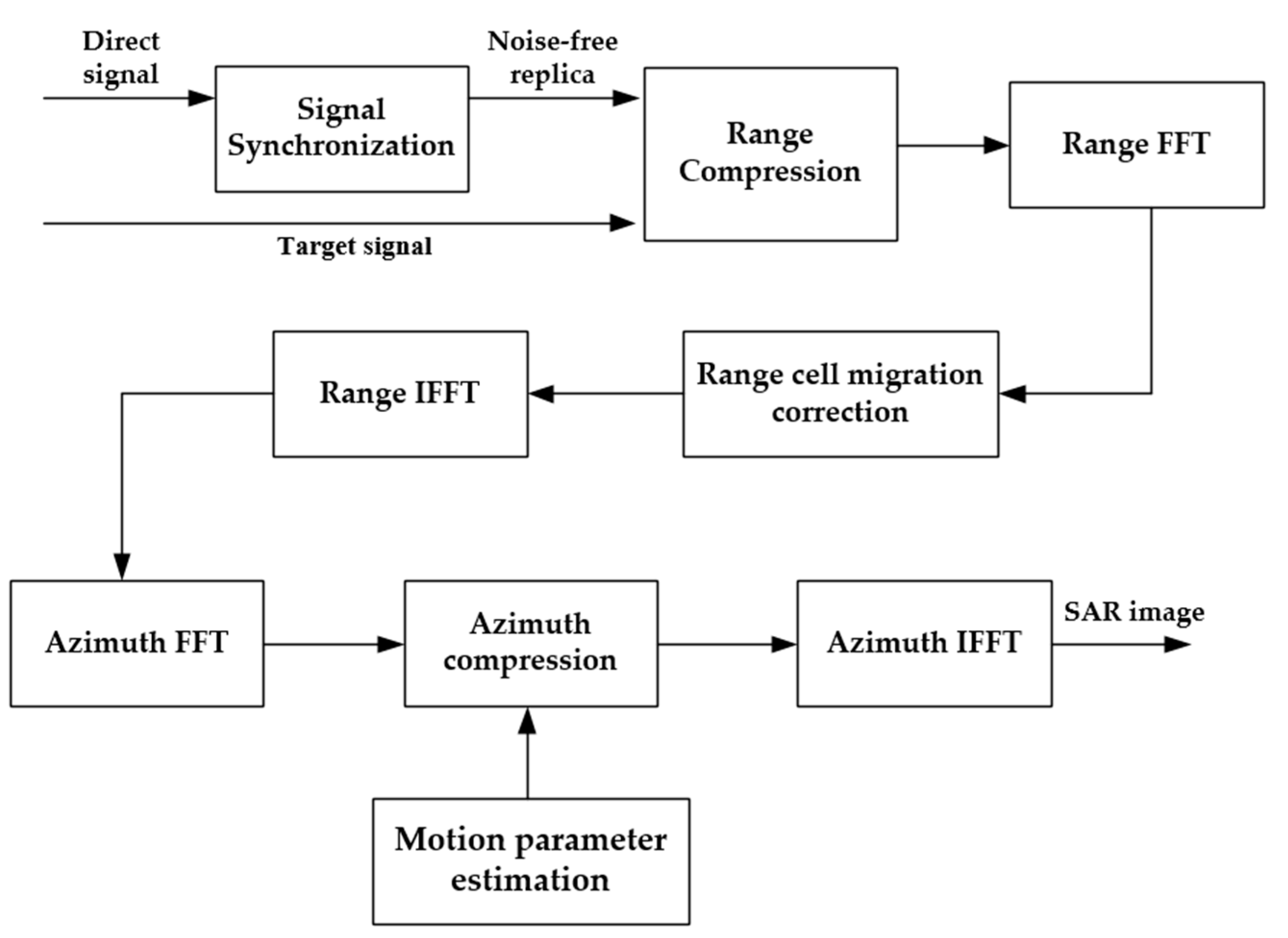
3. Moving Target Image Formation Algorithm
3.1. Signal Synchronization and Signal Model
3.2. Range Compression
- The reference signal and the target signal have the same navigation data within the range of 6000 km [33].
- has eliminated the total phase errors, respectively, induced by the atmospheric factors and the receiver errors due to the similar atmospheric factors and the shared oscillator in the RC and SC [34].
- can be neglected considering the low Doppler frequencies induced by the moving target during the PRI [34].
3.3. Range Cell Migration Correction
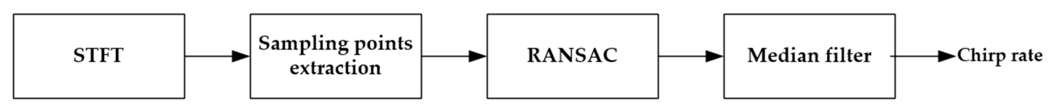
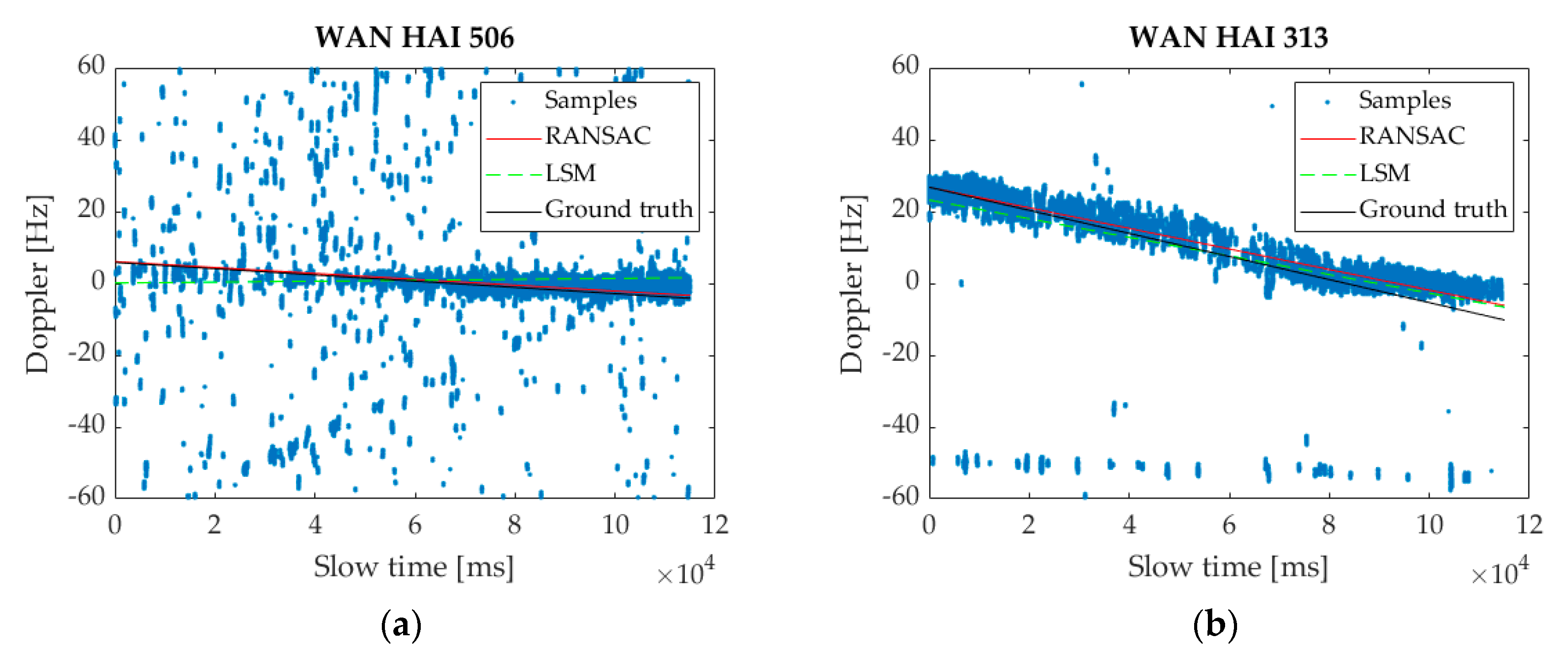
3.4. Motion Parameter Estimation
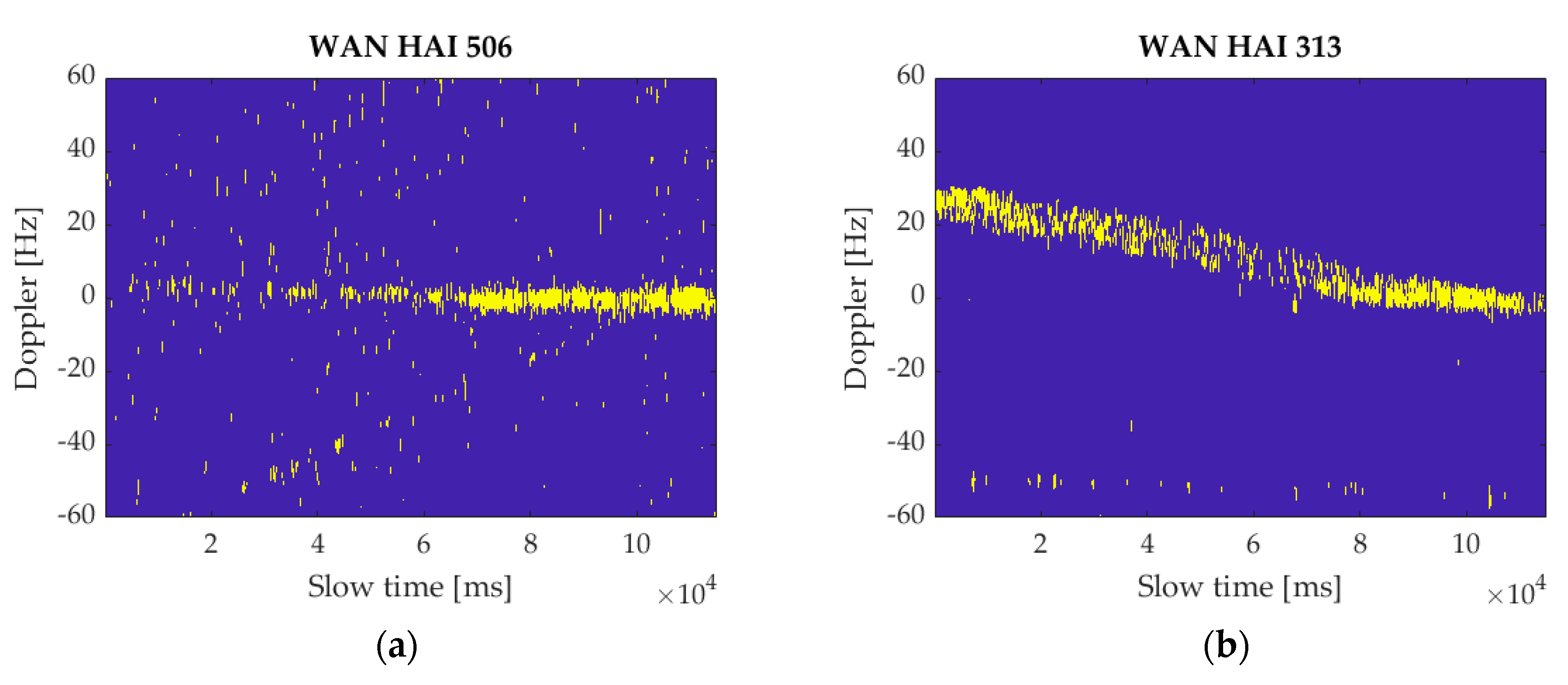
3.4.1. STFT and Time-Frequency Sampling Point Extraction
3.4.2. RANSAC and Median Filter
- Because the chirp rate in (22) is always negative, two points with the positive slope value are not considered.
- The maximum considered chirp rate value can be set to limit the point selection region.
- Because of the long observation time, two points with respect to the time axis should be selected as far away as possible so that the line can fit more sampling points.
3.5. Azimuth Compression
4. Experimental Results
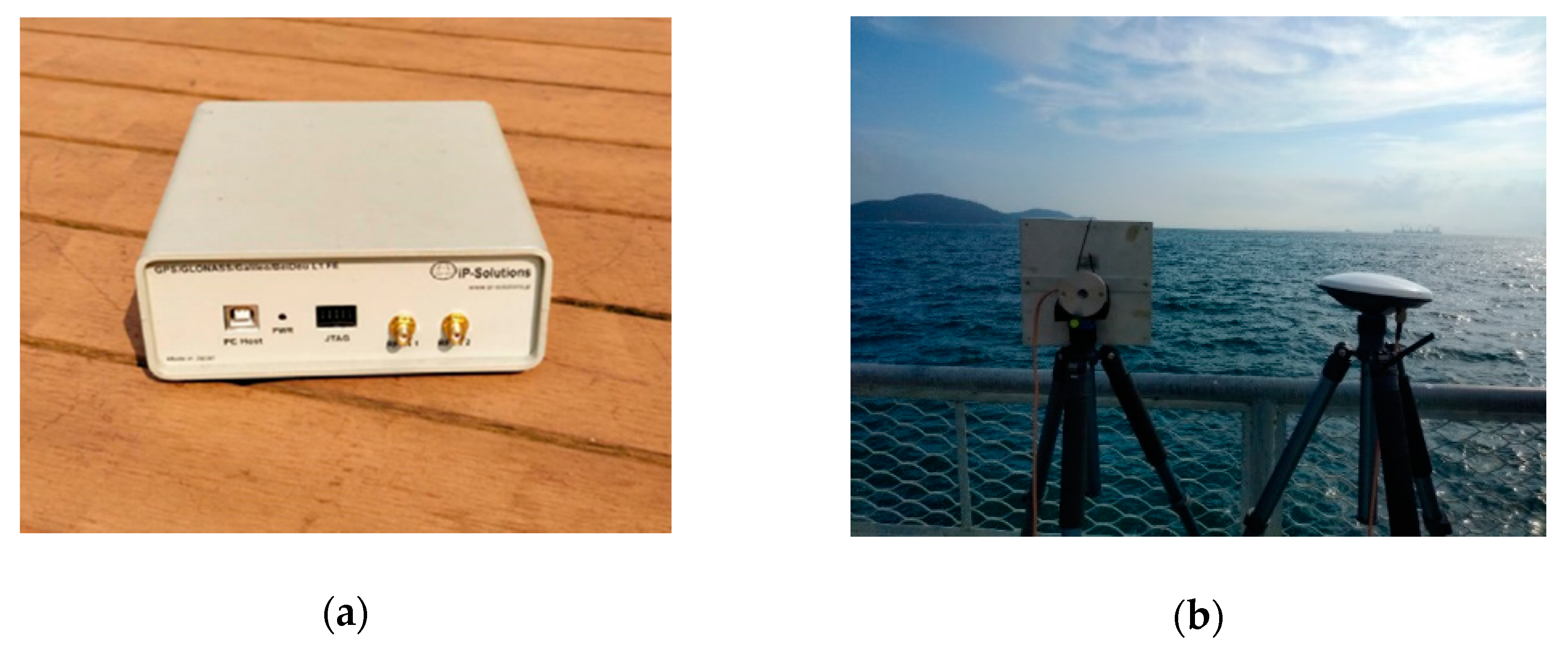
4.1. Experimental Setup
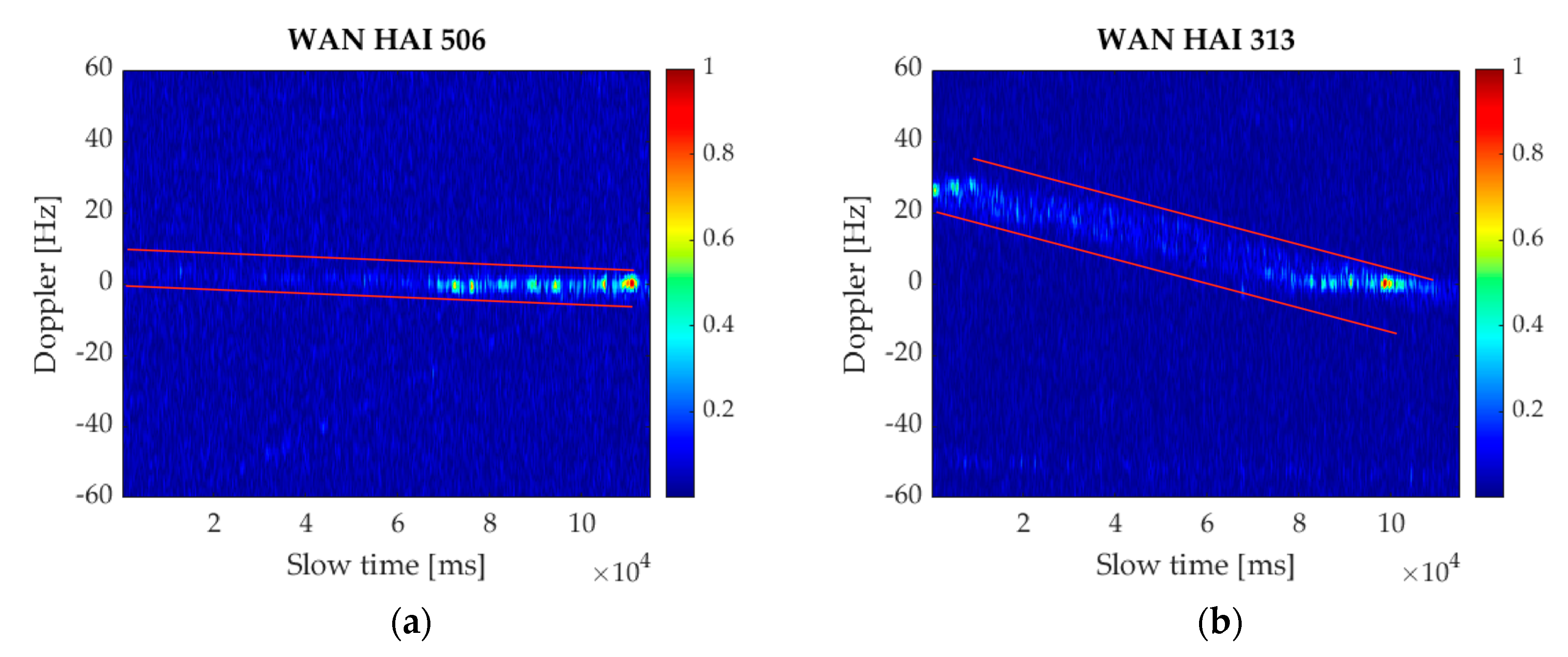
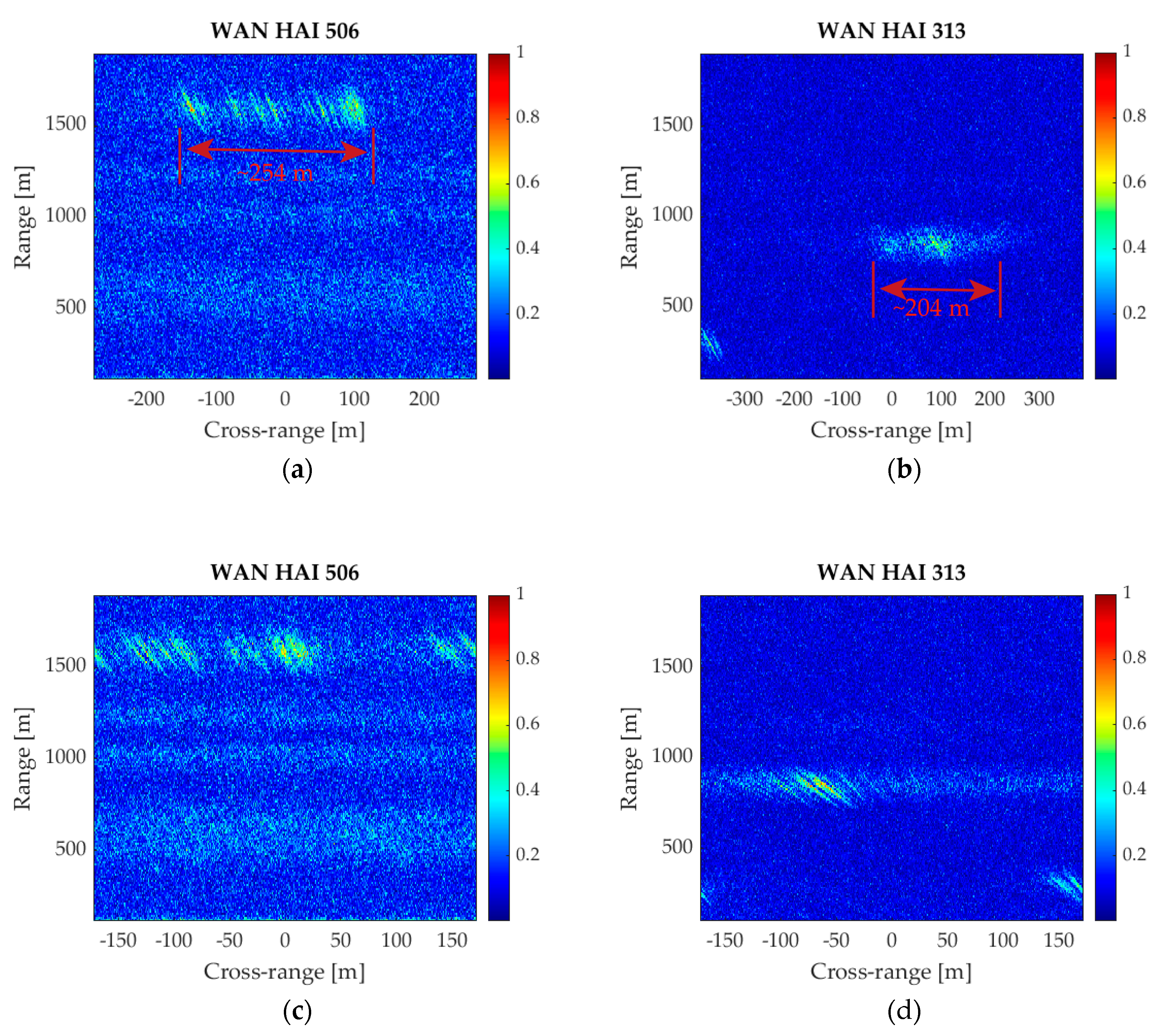
4.2. Velocity Estimation Results and SAR Images
5. Discussion
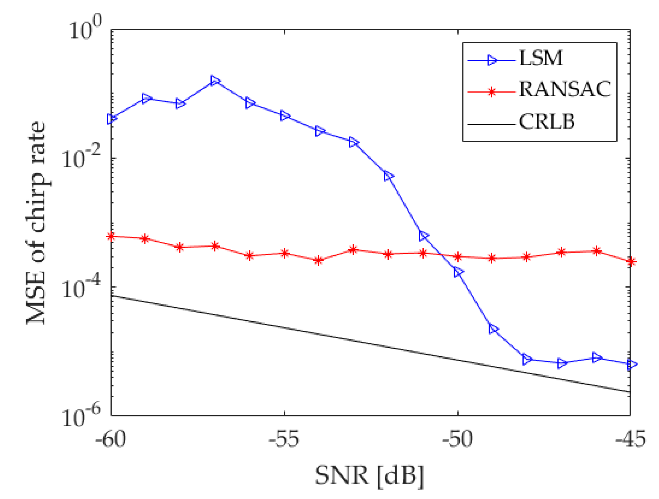
5.1. Mean Square Error of the Chirp Rate Estimation Method
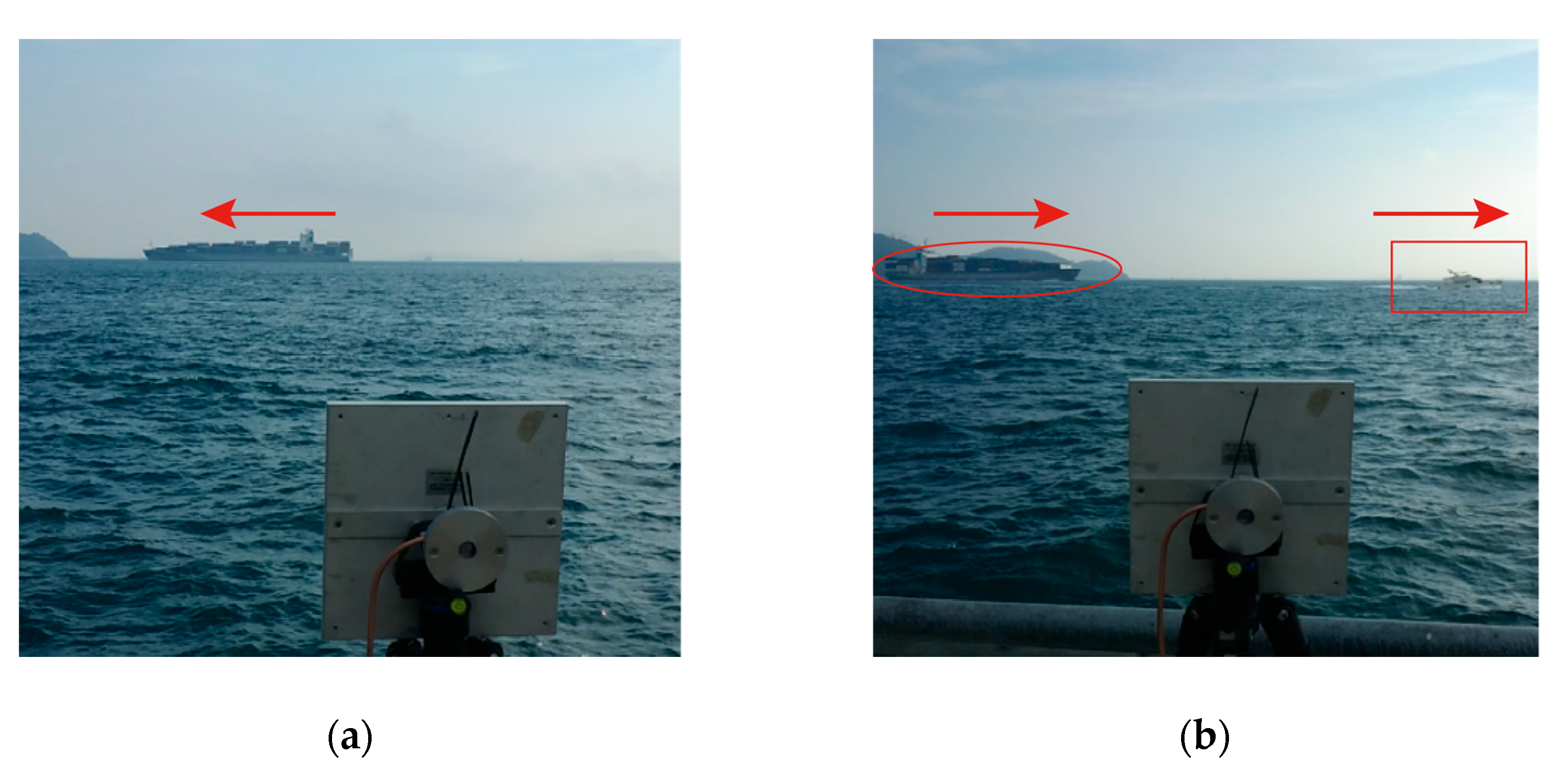
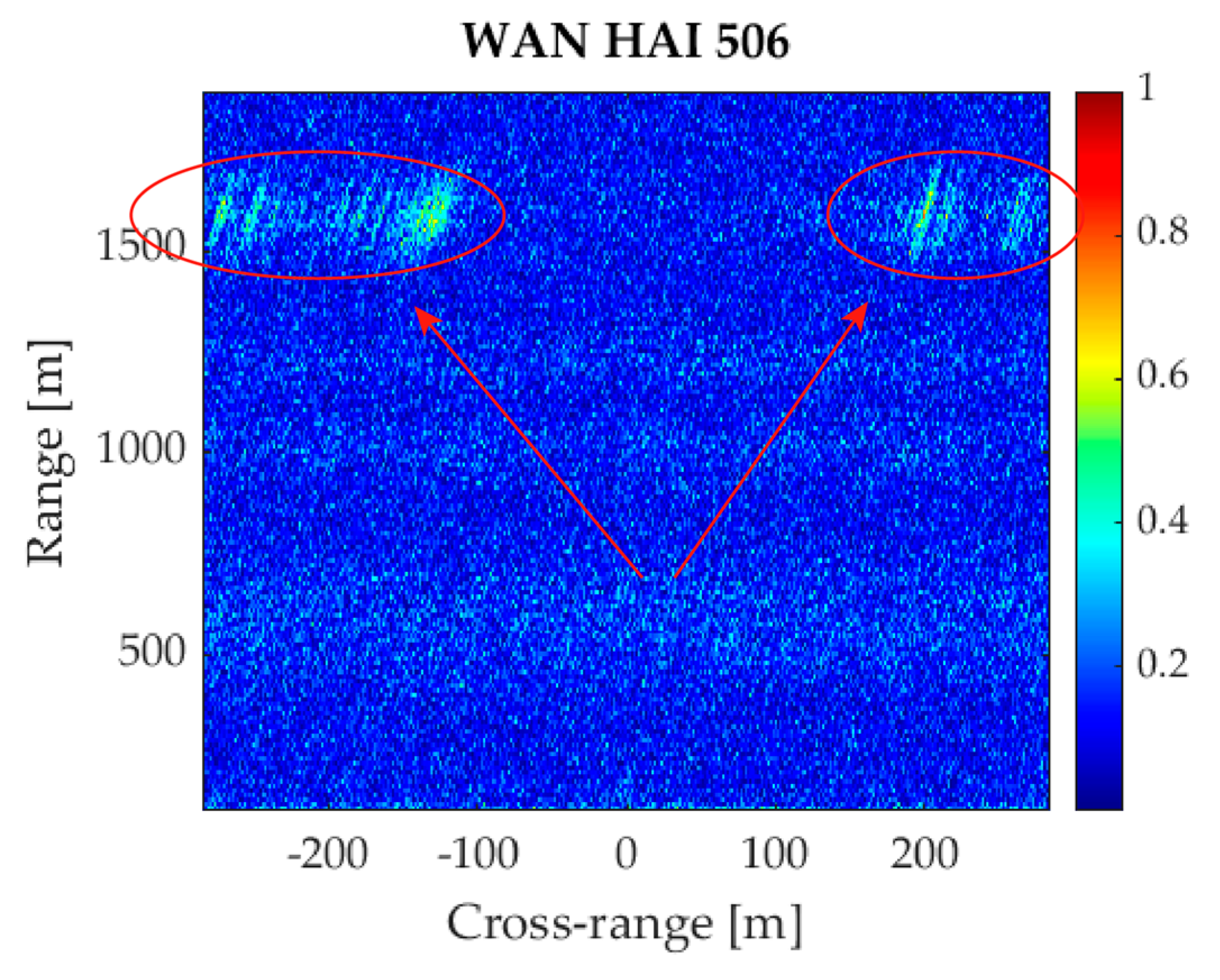
5.2. Target’s Moving Direction Determination
6. Conclusions
Author Contributions
Funding
Conflicts of Interest
References
- Gromek, D.; Kulpa, K.; Samczynski, P. Experimental Results of Passive SAR Imaging Using DVB-T Illuminators of Opportunity. IEEE Geosci. Remote. Sens. Lett. 2016, 13, 1124–1128. [Google Scholar] [CrossRef]
- Colone, F.; Pastina, D.; Marongiu, V. VHF Cross-Range Profiling of Aerial Targets Via Passive ISAR: Signal Processing Schemes and Experimental Results. IEEE Trans. Aerosp. Electron. Syst. 2017, 53, 218–235. [Google Scholar] [CrossRef]
- Zemmari, R.; Nickel, U.; Broetje, M.; Battistello, G. GSM passive coherent location system: Performance prediction and measurement evaluation. IET Radar Sonar Navig. 2014, 8, 94–105. [Google Scholar] [CrossRef]
- Cherniakov, M. Space-surface bistatic synthetic aperture radar: Prospective and problems. In Proceedings of the IEE Conference Publication, Edinburgh, UK, 15–17 October 2002; pp. 22–25. [Google Scholar]
- Antoniou, M.; Cherniakov, M. GNSS-based bistatic SAR: A signal processing view. EURASIP J. Adv. Signal Process. 2013, 2013, 98. [Google Scholar] [CrossRef]
- Antoniou, M.; Cherniakov, M.; Ma, H. Space-surface bistatic synthetic aperture radar with navigation satellite transmissions: A review. Sci. China Inf. Sci. 2015, 58, 1–20. [Google Scholar] [CrossRef] [Green Version]
- Antoniou, M.; Saini, R.; Cherniakov, M. Results of a Space-Surface Bistatic SAR Image Formation Algorithm. IEEE Trans. Geosci. Remote. Sens. 2007, 45, 3359–3371. [Google Scholar] [CrossRef]
- Antoniou, M.; Cherniakov, M.; Hu, C. Space-Surface Bistatic SAR Image Formation Algorithms. IEEE Trans. Geosci. Remote. Sens. 2009, 47, 1827–1843. [Google Scholar] [CrossRef]
- Antoniou, M.; Zhang, Q.; Cherniakov, M.; Hong, Z.; Zhangfan, Z.; Zuo, R. Passive bistatic synthetic aperture radar imaging with Galileo transmitters and a moving receiver: Experimental demonstration. IET Radar Sonar Navig. 2013, 7, 985–993. [Google Scholar] [CrossRef]
- Zeng, T.; Liu, F.; Antoniou, M.; Cherniakov, M. GNSS-based BiSAR imaging using modified range migration algorithm. Sci. China Inf. Sci. 2015, 58, 1–13. [Google Scholar] [CrossRef]
- Zeng, H.-C.; Wang, P.-B.; Chen, J.; Liu, W.; Ge, L.; Yang, W. A Novel General Imaging Formation Algorithm for GNSS-Based Bistatic SAR. Sensors 2016, 16, 294. [Google Scholar] [CrossRef]
- Zeng, Z.; Shi, Z.; Xing, S.; Pan, Y. A Fourier-Based Image Formation Algorithm for Geo-Stationary GNSS-Based Bistatic Forward-Looking Synthetic Aperture Radar. Sensors 2019, 19, 1965. [Google Scholar] [CrossRef] [PubMed] [Green Version]
- Zhou, X.-K.; Chen, J.; Wang, P.; Zeng, H.-C.; Fang, Y.; Men, Z.-R.; Liu, W. An Efficient Imaging Algorithm for GNSS-R Bi-Static SAR. Remote. Sens. 2019, 11, 2945. [Google Scholar] [CrossRef] [Green Version]
- Liu, F.; Antoniou, M.; Zeng, Z.; Cherniakov, M. Coherent Change Detection Using Passive GNSS-Based BSAR: Experimental Proof of Concept. IEEE Trans. Geosci. Remote. Sens. 2013, 51, 4544–4555. [Google Scholar] [CrossRef]
- Zhang, Q.; Antoniou, M.; Chang, W.; Cherniakov, M. Spatial Decorrelation in GNSS-Based SAR Coherent Change Detection. IEEE Trans. Geosci. Remote. Sens. 2014, 53, 219–228. [Google Scholar] [CrossRef]
- Liu, F.; Fan, X.; Zhang, L.; Zhang, T.; Liu, Q. GNSS-based SAR for urban area imaging: Topology optimization and experimental confirmation. Int. J. Remote. Sens. 2019, 40, 4668–4682. [Google Scholar] [CrossRef]
- Ma, H.; Antoniou, M.; Cherniakov, M. Passive GNSS-Based SAR Resolution Improvement Using Joint Galileo E5 Signals. IEEE Geosci. Remote. Sens. Lett. 2015, 12, 1640–1644. [Google Scholar] [CrossRef]
- Zheng, Y.; Yang, Y.; Chen, W. A Novel Range Compression Algorithm for Resolution Enhancement in GNSS-SARs. Sensors 2017, 17, 1496. [Google Scholar] [CrossRef] [Green Version]
- Zeng, Z.; Shi, Z.; Zhou, Y.; Chen, Y.; Pan, Y. An Improved Pre-Processing Algorithm for Resolution Optimization in Galileo-Based Bistatic SAR. IEEE Access 2019, 7, 122972–122981. [Google Scholar] [CrossRef]
- Fang, Y.; Chen, J.; Wang, P.; Zhou, X. An Image Formation Algorithm for Bistatic SAR Using GNSS Signal With Improved Range Resolution. IEEE Access 2020, 8, 80333–80346. [Google Scholar] [CrossRef]
- Sun, G.-C.; Xing, M.; Xia, X.-G.; Wu, Y.; Bao, Z. Robust Ground Moving-Target Imaging Using Deramp–Keystone Processing. IEEE Trans. Geosci. Remote. Sens. 2012, 51, 966–982. [Google Scholar] [CrossRef]
- Yang, J.; Liu, C.; Wang, Y. Detection and Imaging of Ground Moving Targets With Real SAR Data. IEEE Trans. Geosci. Remote. Sens. 2014, 53, 920–932. [Google Scholar] [CrossRef]
- Pelich, R.; Longepe, N.; Mercier, G.; Hajduch, G.; Garello, R. Vessel Refocusing and Velocity Estimation on SAR Imagery Using the Fractional Fourier Transform. IEEE Trans. Geosci. Remote. Sens. 2015, 54, 1670–1684. [Google Scholar] [CrossRef]
- Li, Z.; Wu, J.; Liu, Z.; Huang, Y.; Yang, H.; Yang, J. An Optimal 2-D Spectrum Matching Method for SAR Ground Moving Target Imaging. IEEE Trans. Geosci. Remote. Sens. 2018, 56, 5961–5974. [Google Scholar] [CrossRef]
- Colone, F.; Pastina, D.; Falcone, P.; Lombardo, P. WiFi-Based Passive ISAR for High-Resolution Cross-Range Profiling of Moving Targets. IEEE Trans. Geosci. Remote. Sens. 2013, 52, 3486–3501. [Google Scholar] [CrossRef]
- Pisciottano, I.; Cristallini, D.; Pastina, D. Maritime target imaging via simultaneous DVB-T and DVB-S passive ISAR. IET Radar Sonar Navig. 2019, 13, 1479–1487. [Google Scholar] [CrossRef]
- Pieralice, F.; Santi, F.; Pastina, D.; Antoniou, M.; Cherniakov, M. Ship targets feature extraction with GNSS-based passive radar via ISAR approaches: Preliminary experimental study. In Proceedings of the EUSAR 2018; 12th European Conference on Synthetic Aperture Radar, Aachen, Germany, 4–7 June 2018; pp. 1–5. [Google Scholar]
- Santi, F.; Pieralice, F.; Pastina, D.; Antoniou, M.; Cherniakov, M. Passive radar imagery of ship targets by using navigation satellites transmitters of opportunity. In Proceedings of the 20th International Radar Symposium (IRS), Ulm, Germany, 26–28 June 2019; pp. 1–10. [Google Scholar] [CrossRef]
- Martorella, M.; Pastina, D.; Berizzi, F.; Lombardo, P. Spaceborne Radar Imaging of Maritime Moving Targets With the Cosmo-SkyMed SAR System. IEEE J. Sel. Top. Appl. Earth Obs. Remote. Sens. 2014, 7, 2797–2810. [Google Scholar] [CrossRef]
- Perry, R.; DiPietro, R.; Fante, R. SAR imaging of moving targets. IEEE Trans. Aerosp. Electron. Syst. 1999, 35, 188–200. [Google Scholar] [CrossRef]
- Fischler, M.; Bolles, R. Random sample consensus: A paradigm for model fitting with applications to image analysis and automated cartography. Commun. ACM 1981, 24, 381–395. [Google Scholar] [CrossRef]
- Yang, Y.; Zheng, Y.; Yu, W.; Chen, W.; Weng, D. Deformation monitoring using GNSS-R technology. Adv. Space Res. 2019, 63, 3303–3314. [Google Scholar] [CrossRef]
- Zeng, Z. Passive Bistatic SAR with GNSS Transmitter and a Stationary Receiver. Ph.D. Thesis, University of Birmingham, Birmingham, UK, 2013. [Google Scholar]
- Pastina, D.; Santi, F.; Pieralice, F.; Bucciarelli, M.; Ma, H.; Tzagkas, D.; Antoniou, M.; Cherniakov, M. Maritime Moving Target Long Time Integration for GNSS-Based Passive Bistatic Radar. IEEE Trans. Aerosp. Electron. Syst. 2018, 54, 3060–3083. [Google Scholar] [CrossRef] [Green Version]
- Wood, J.; Barry, D. Radon transformation of time-frequency distributions for analysis of multicomponent signals. IEEE Trans. Signal Process. 1994, 42, 3166–3177. [Google Scholar] [CrossRef]
- Xia, X.-G. Discrete chirp-Fourier transform and its application to chirp rate estimation. IEEE Trans. Signal Process. 2000, 48, 3122–3133. [Google Scholar] [CrossRef] [Green Version]
- Ozaktas, H.; Arikan, O.; Kutay, M.; Bozdagt, G. Digital computation of the fractional Fourier transform. IEEE Trans. Signal Process. 1996, 44, 2141–2150. [Google Scholar] [CrossRef] [Green Version]
- Cumming, I.G.; Wong, F.H. Digital Processing of Synthetic Aperture Radar Data: Algorithms and Implementation; Artech House Print on Demand: London, UK, 2005. [Google Scholar]
- Di Simone, A.; Braca, P.; Millefiori, L.M.; Willett, P. Ship detection using GNSS-reflectometry in backscattering configuration. In Proceedings of the 2018 IEEE Radar Conference (RadarConf18), Oklahoma City, OK, USA, 23–27 April 2018; pp. 1589–1593. [Google Scholar]
- Peleg, S.; Porat, B. The Cramer-Rao lower bound for signals with constant amplitude and polynomial phase. IEEE Trans. Signal Process. 1991, 39, 749–752. [Google Scholar] [CrossRef]


| Parameters | Values |
|---|---|
| Coordinates of the receiver | (0, 0, 0) |
| Satellite-to-receiver range (Rb) | 20,000 km |
| Satellite elevation angle (α) | 0°, 30°, 45°, 60° |
| Local azimuth angle (az) | 0°, 30°, 45°, 60° |
| Radar antenna beam angle (θbw) | 10° |
| Target-to-receiver vertical range (Rs) | 500–5000 m |
| Half-length of the synthetic aperture (L) | Rs × tan(θbw/2) |
| Coordinates of the receiver | (0, 0, 0) |
| Satellite-to-receiver range (Rb) | 20,000 km |
| Parameters | Values |
|---|---|
| Sampling frequency | 16.368 MHz |
| Pulse repetition frequency (PRF) | 1000 Hz |
| Observation time | 120 s |
| Azimuth angle of antenna pointing direction | 239.7° |
| Length of the analyzing window (T) | 2048 ms |
| Sampling points extraction threshold | 0.1 |
| The maximum RANSAC iteration number | 200 |
| The tolerance threshold | (PRF/T) × 3 |
| The proportion of the minimum number of inliers | 7.5% |
| Name | Length | Speed | Vertical Range | PRN/Elev/Az |
|---|---|---|---|---|
| WAN HAI 506 | 269 m | 4.94 m/s | 1663.7 m | 3/40°/68° |
| WAN HAI 313 | 213 m | 7.21 m/s | 938.6 m | 22/19°/46° |
| Name | Est. Chirp Rate | Est. Velocity | AIS Chirp Rate | AIS Velocity |
|---|---|---|---|---|
| WAN HAI 506 | −0.082 Hz/s | 4.81 m/s | −0.087 Hz/s | 4.94 Hz/s |
| WAN HAI 313 | −0.286 Hz/s | 6.81 m/s | −0.321 Hz/s | 7.21 Hz/s |
| Parameters | Values | |
|---|---|---|
| Boltzmann constant | 1.38 × 10²³ | |
| Environment | Temperature | 300 K |
| Power density on the ground | −153 W/m2 | |
| Observation time | 16,384 ms | |
| Antenna gain | 20 dB | |
| Receiver | Receiver noise bandwidth | 1.023 MHz |
| Receiver Noise figure | 2.03 dB | |
| Target | Target’s velocity | 7.47 m/s |
| Target-to-receiver vertical range | 1000 m |
Publisher’s Note: MDPI stays neutral with regard to jurisdictional claims in published maps and institutional affiliations. |
© 2020 by the authors. Licensee MDPI, Basel, Switzerland. This article is an open access article distributed under the terms and conditions of the Creative Commons Attribution (CC BY) license (http://creativecommons.org/licenses/by/4.0/).
Share and Cite
He, Z.-Y.; Yang, Y.; Chen, W.; Weng, D.-J. Moving Target Imaging Using GNSS-Based Passive Bistatic Synthetic Aperture Radar. Remote Sens. 2020, 12, 3356. https://doi.org/10.3390/rs12203356
He Z-Y, Yang Y, Chen W, Weng D-J. Moving Target Imaging Using GNSS-Based Passive Bistatic Synthetic Aperture Radar. Remote Sensing. 2020; 12(20):3356. https://doi.org/10.3390/rs12203356
Chicago/Turabian StyleHe, Zhen-Yu, Yang Yang, Wu Chen, and Duo-Jie Weng. 2020. "Moving Target Imaging Using GNSS-Based Passive Bistatic Synthetic Aperture Radar" Remote Sensing 12, no. 20: 3356. https://doi.org/10.3390/rs12203356