Simulation of the Dynamic Water Storage and Its Gravitational Effect in the Head Region of Three Gorges Reservoir Using Imageries of Gaofen-1

Abstract

The construction of a high-resolution dynamic water storage model, driven by the mass load of the huge water storage of the Three Gorges Reservoir (TGR), is the necessary basic data for accurately simulating changes in the geophysical field, e.g., gravity, crustal deformation, and stress. However, previously established models cannot meet the needs of accurately simulating the impoundment effects of TGR, because these models were simplified and approximated and did not consider the variation of river boundaries caused by water level changes. In this study, we combined high-resolution Gaofen-1 (GF-1) satellite imageries and real-time water level in front of the dam and extracted 31 river boundaries of the head region of TGR between the lowest (145 m) and the highest (175 m) impoundment stages based on the Normalized Differential Water Index (NDWI) and threshold segmentation from Otsu method. Developed dynamic water storage model based on higher-resolution GF-1 data can show the true river boundary changes more exactly, especially in local areas. Compared to the previous approximate models, the model that we constructed accurately depicts the boundary distribution information of the different impoundment stages. Moreover, we simulated TGR-induced gravitational effects based on the high-precision forward modeling of the dynamic water storage model (i.e., considering changes of dynamic water area and water level). The theoretical modelled results are consistent with in situ gravity measurements with the difference mainly within 10 μGal. Our results indicate that water storage variations of TGR mainly affect the gravity field response within 1000 m of the reservoir bank with its maximum amplitude up to several hundred μGal. The dynamic water storage and its simulation results of gravitational effects can effectively eliminate the impact of surface water load driven by the TGR under human control and greatly improve the signal-to-noise ratio of regional gravity observational data. Thus, this work will be beneficial in the application of geophysical and geodetic monitoring aimed to comprehensively track the local and regional geological structural stability, e.g., artificial reservoir induced earthquake and landslide.

1. Introduction

Determining the Earth’s surface hydrological processes of terrestrial water storage or human-induced water storage is considered a recent interest because the processes reflect the information of modern climate cycles changes [1]. The Three Gorges Reservoir (TGR) in China, covering the section from Yichang to Chongqing of Yangtze River basin (Figure 1), is one of the largest reservoirs in the world and a typical representative of man-made terrestrial water circulation [2,3]. Since the impoundment successfully reached its largest capacity (i.e., ~175 m water level) in 2008, the water level of the reservoir is perennially controlled in the periodic fluctuation between 145 m and 175 m for meeting the needs of flood control and irrigation in its lower reaches of the Yangtze River basin.

The huge water storage change caused by impoundment in the TGR and its impacts on the regional environment [4,5,6] and accompanying variations in crustal load and deformation due to the water level rising and falling have been the focus issues for a long time [7,8]. The result of water storage fluctuation is considered as important inducing factors for geological hazards such as reservoir earthquakes and landslides around the TGR [7,8]. Therefore, constructing a water storage model of the TGR is necessary to estimate the impacts due to water storage change. Models established previously [9,10,11,12] were relatively simple, and the variation of river boundaries caused by the impoundment was not considered. Since the change of reservoir water level has great influence on the nearshore area, where numerous landslides and earthquakes occurred during the impoundment process of the TGR [13,14], developing more accurate models is helpful to further understand the water storage of the TGR in different impoundment periods and dynamically analyze its impacts in time.

Previous models were constructed based on Digital Elevation Model (DEM) data. The Shuttle Radar Topographic Mission (SRTM), with a ground resolution of ~90 m and a vertical error of less than 16 m at a 90% confidence level [15,16], was widely used for determining TGR modelling data in previous studies [9,10,11,12]. Because the SRTM DEM’s lower spatial resolution may result in large uncertainties and does not provide the information of seasonable water boundary lines [9], combining it with high resolution satellite imageries is of benefit to tack water boundary lines at different water levels, establishing a more accuracy and dynamic water storage model. Satellite imageries with high spatio-temporal resolution can provide detailed information for target identification. They are frequently used for the monitoring of river basin evolution [17,18], in hydrodynamic process modeling [19,20], and in the analysis of characteristic changes of water bodies [21,22,23]. The Gaofen-1 (GF-1) is the first satellite in the series of China High-resolution Earth Observation Satellites (CHEOS). Imageries from GF-1 have a favorable spatio-temporal resolution with revisit period of 3 to 5 days and ground resolution of ~2 m and have been used for classifying water bodies [22,23] and extracting water information [22,24,25,26].

Geophysical and geodetic monitoring system usually is employed in large reservoirs aiming to comprehensively investigate the local and regional geological structural stability. The gravitational effects derived from the variation of water storage in a reservoir are sensitive geophysical responses of the water mass variation and water leakage of the reservoir as well as crustal deformation around the reservoir. As an effective monitoring approach, high precision gravity surveys on the ground and in the space are frequently applied to investigate the mass migration on the surface of the Earth [2,3,4,6,11,12,27,28,29]. The simulation of the gravitational effect generated by the water storage change is an essential step to effectively distinguish causes of the local and regional geological structural stability (e.g., deformation, water leakage) from superposed signals. An accuracy water storage model of the TGR represents a good opportunity to detailly investigate gravitational responses in this process [3].

In this study, we used GF-1 satellite imageries to extract the water boundaries at water levels of ~145 m and ~175 m over the head region of the TGR (from Zigui to Badong, see Figure 1). Subsequently, we acquired the water boundary data at different water levels between 145 m and 175 m, and used obtained water boundary data to simulate gravitational effects generated by the dynamic water storage at various water levels. Then, we used the method of polyhedral integral of complex body to calculate the change of the gravity field based on the established dynamic water storage model. Simulated results were verified by ground gravity data measurements (i.e., A10 absolute gravity).

2. Data and Methods

Construction of dynamic water storage model is mainly divided into three steps: (1) selecting imageries and doing data preprocessing, (2) extracting the water boundaries at the highest and the lowest water levels based on post-processing satellite imageries, and (3) determining water boundaries in middle water levels between the highest and lowest water levels by interpolating and then constructing a series of models, which have water bodies with complex reservoir bank surface and can reflect water storages in different impoundment phases in the front of TGR dam. Corresponding gravitation effects caused by dynamic water models can be presented by the algorithm based on the exact theory.

2.1. GF-1 Imageries and Data Preprocessing

The GF-1′s payload has high spatial and temporal resolutions and a wide swath width (

Table 1. General information of the payload and specification of the GF-1 satellite.

Sensor	Band No.	Spectral Range (μm)	Spatial Resolution (m)	Swath Width (km)	Repeat Cycle (Days)	Regression Cycle (Days)
Panchromatic camera		0.45–0.89	2	60 (2 cameras combined)	3–5	41
Multispectral camera	B1	0.45–0.52	8
	B2	0.52–0.59
	B3	0.63–0.69
	B4	0.77–0.89

). Fusing panchromatic imagery data (2 m resolution) and multispectral imagery data (8 m resolution), the product of the GF-1 is capable of identifying meticulous water boundaries and is easily used for the visual interpretation. Here, raw panchromatic and multispectral imageries need to go through a series of preprocessing before application. For removing the geometrical distortions, we applied the ASTER GDEM to orthorectify selected imageries. ASTER GDEM is a newer global DEM and has a ground resolution of ~30 m (https://lpdaac.usgs.gov/products/astgtmv002/). The imagery data preprocessing procedure shown in Figure 2 was completed using the ArcMap software (available at https://desktop.arcgis.com/zh-cn/arcmap/).

Satellite imagery compatible to our task needs to be selected from the large dataset of GF-1. The water level of the TGR varies throughout the whole year, but it usually stays at high water level for power generation in the winter months (November to February) and stays at low water level for flood control (June to August) [4]. Imageries acquired in these two periods are acceptable, except that there are a lot of clouds over the study area. Imageries acquired in the periods in which the water level quickly rises (September to October) and quickly falls (March to May) are not acceptable because those imageries cannot provide clear water boundaries due to the water level varying rapidly. Therefore, time frame for imagery acquisition is crucial in the study. We finally selected 11 imageries over the study area with little cloud cover in the period when water levels were about 145 m and 175 m (

Table 2. The selected GF-1 imageries at different impoundment periods.

Impoundment Period	Imagery No	Product ID	Center Coordinate (WGS84)	Acquired Date	Cloud Cover (%)	Water Level (m)
Low water level (June to August)	1	2446123	30°43′, 110°58′	27 June 2017	7	145.66
	2	2446067	31°04′, 110°40′		14
	3	96759	31°17′, 110°28′	8 August 2015	8	145.48
	4	96760	31°00′, 110°24′		13
High water level (November to February)	5	177856	30°51′, 110°16′	6 December 2013	0	174.40
	6	126992	30°47′, 110°38′		0
	7	127087	31°08′, 110°21′		0
	8	1939558	31°00′, 111°01′	5 November 2016	0	174.40
	9	1939560	30°43′, 110°57′		0
	10	1939455	31°04′, 110°40′		0
	11	1939462	31°20′, 110°44′		0

).

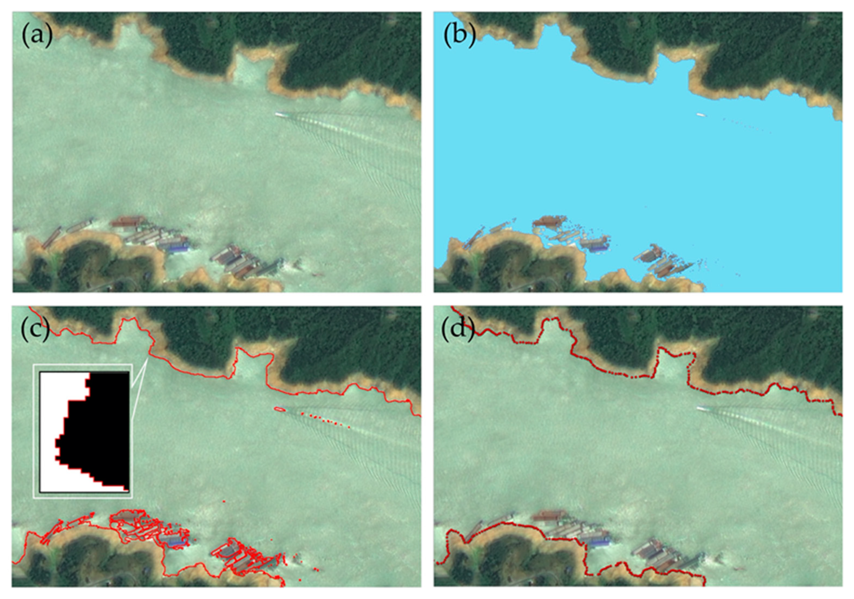
2.2. Extraction of Water Boundaries

Water reflectance is generally rather low (4–5%) in the visible light range. Even though it is relatively high in the blue-green band, water reflectance is lower in the near infrared band and has a downtrend with increase in light wavelength. Hence, water bodies are mostly dark in the remote sensing imageries, and it is useful to distinguish the water body from other ground objects in the spectrum. In order to classify water targets from remote sense imageries, McFeeters [30] proposed the Normalized Differential Water Index (NDWI) applied to identify water bodies according to the difference of normalized ratio index of the green band and the near-infrared band. This approach has been previously used for distinguishing and extracting the water boundaries [22,31,32,33]. We use NDWI [30] to distinguish water bodies by applying the following equation:

$$NDWI=\frac{B2-B4}{B2+B4}$$

(1)

where B2 and B4 denote reflectance in blue-green band and near-infrared band, respectively. NDWI can enhance the difference between B2 and B4 and effectively separate water from other land covers, and thereby, it can be taken as an indicator for discriminating water and non-water features.

The water boundary extraction of the corrected fused multispectral imagery can be implemented by the following steps (Figure 3): (1) calculating the NDWI imagery, (2) using the Otsu method [34] to get the optimal threshold and segment the water body information, (3) through the local visual interpretation adjustment, we can get the corrected water boundaries.

Figure 4 shows a part of the fused multispectral imagery (Figure 4a) and the NDWI imagery (Figure 4b). It is further necessary for selecting an appropriate threshold to distinguish water from other objects in NDWI imagery. The Otsu method [34] is considered as an efficient approach to perform binarized segmentation that is usually applied to identify water bodies or non-water bodies [22].

The threshold value is calculated based on the rule of maximum between-class variance and minimum within-class variance in the Otsu method. Following this principle, assume [a, b] as the range of index value in NDWI imagery; any threshold t (a ≤ t ≤ b) may divide indices into two categories, i.e., indices are attributed to the water category as they are larger than t, and others are attributed to the non-water category. The optimal threshold should be calculated in equations by following:

$$\{\begin{array}{l}{\sigma }_t^2=(P_{nw}\cdot {(M_{nw}-M)}^2+P\cdot {(M_w-M)}^2\\ M=P_{nw}\cdot M_{nw}+P_w\cdot M_w\\ P_{nw}+P_w=1\end{array}$$

(2)

where σ_t is the between-class variance with respect to t; P_w (water) and P_nw (non-water) are probabilities of pixel units divided into two categories respectively, and M_w (water) and M_nw (non-water) are their average NDWI values. Given different t for test, the optimal threshold T_opt can be determined by:

$$T_{opt}=\underset{a\le t\le b}{ArgMax}\left\{{\sigma }_t^2\right\}$$

(3)

The spectrum divergence among different imageries is usually inconsistent due to different observation periods and locations. Thus, selecting an optimal threshold for each imagery is required. We change threshold t with an interval of 0.01 and iteratively search maximum between-class variances for every imagery. Achieved optimal thresholds for imageries used in this study are listed in

Table 3. The optimal threshold of selected GF-1 imageries by Otsu method.

Imagery No.	1	2	3	4	5	6	7	8	9	10	11
Optimal threshold	0.23	0.47	0.48	0.47	0.31	0.20	0.34	0.13	0.14	0.07	0.01

.

Binarized imagery, according to the achieved optimal threshold, can be obtained by applying the following formula:

$$A_w=\{\begin{array}{c}1,\\ 0,\end{array}\begin{array}{l}\hspace{0.17em}water\hspace{1em}\hspace{1em}(\mathit{NDWI}\ge T_{opt})\\ \hspace{0.17em}\mathit{non}\text{-}\mathit{water}\hspace{0.17em}\hspace{0.17em}({\mathit{NDWI}<\mathit{T}}_{opt})\end{array}$$

(4)

where A_w denotes the attribution value of water in the binarized segmentation imagery. Water boundaries at pixel level can be easily extracted from a binarized imagery through the conversion from raster imagery to vector map. Boundary lines are composed of segments that connect nodes between adjacent water and non-water pixels, in which vector boundary line dataset consists of node coordinates. Figure 4c shows a part of binarized imagery transformed from a NDWI imagery in this study.

Although algorithms for the automatic target identification are efficient and successful, they are often influenced by interferences such as mountain shadows, ships, bridges, and floating objects (Figure 4c). Accordingly, further corrections should be manually accomplished based on the visual inspection of the imageries as a complement [35,36,37] (Figure 4d). The extracted water boundary lines at water levels of about 145 m and 175 m are presented in Figure 5.

2.3. Dynamic Model Construction

Previously applied methods [9,10,11,12] for estimating the difference of water storage in the TGR measured the variation of water volume in which the product between the water surface area of closed water boundary lines (at the lowest or the highest), and the water level difference was taken as the estimation of volume variation. However, riverbank and riverbed topography in the TGR area was not considered. The original terrain of the TGR area, before impoundment, was rough and the details can be seen in Figure 6a. It can be noticed that several underwater hills are not fully submerged during the highest and lowest water levels, while others are only submerged during the highest water levels.

As hills are only flooded at the highest water level (Figure 6a, situation II), the water storage may be miscounted. Acquiring other water boundary lines between the highest and the lowest water level can be helpful in diminishing these impacts and miscounts. Since satellite imageries are unsuitable to acquire water boundary lines during water level rising and falling in the TGR, the interpolation based on the lowest and highest water levels may be a reasonable approach. We simulated the bank terrain between water boundary lines at water levels of 145 m and 175 m by the minimum curvature algorithm in order to consider the topography of the reservoir banks. Intermediate water boundaries were obtained from the simulated surface of banks. Afterwards, the water boundary lines with a uniform interval between the highest and the lowest water levels could be acquired. Figure 6b shows the example near the front of the Three Gorges Dam. The results show that the highest and the lowest water level boundaries well constrain the distribution of the intermediate water level lines. Finally, a reasonable water storage model is obtained and it reflects the dynamic process of gradual changes in water level.

Meticulously divided water boundaries provide more possibilities to construct a detailed water storage model at different water levels in the TGR. According to the obtained water boundary lines, the water body of the TGR was divided into a series of horizontal layers. The partial or total combination of layers represents the water storage at different water levels, and it can be used for the estimation of water load and other geophysical effects at various water levels.

Geometrically, each layer of the water body can be described as a complex shape body closed by two respective horizontal planes on the top and bottom and rough surfaces on two reservoir banks, or it can be defined as a polyhedron. For comprehending the construction of a layer of the water body, we detached the river into a series of small segments.

The layered water body shaped in a polyhedron (e.g., the single-layer water body in Figure 7a represents one layer of the multi-layer model such as Layer 3 in Figure 7b) can be separated into three parts: one quadrilateral prism and two pentahedrons (Figure 7c). The quadrilateral prism is the major part of the layer in the segment. After connecting neighboring quadrilateral prisms in segments, those quadrilateral prisms are combined to a huge polygonal prism, with the consistent area on the top and bottom and a certain thickness along the total river (see the right side in Figure 7d). This is a relatively simple model that allows convenient calculation of its load and gravitational effect. However, this model is not appropriate for total water storage calculation. In that case, pentahedrons on the two reservoir banks need to be considered. For example, each considered pentahedron shape is represented by closed surface with one horizontal plane on the top, three vertical planes on the sides, and one quadrangle facet on the bank.

The volume depends on the bank terrain and the corners (vertexes) of the facet (AHG’B’ or DEF’C’ in Figure 7c) are perhaps non-coplanar, i.e., the body is not an exact pentahedron. By subdividing the facet AHG’B’ into two triangular facets (ΔAB’H and ΔHB’G’), the pentahedron becomes an asymmetric hexahedron or polyhedron, and this assumption is suitable for all these bodies on the bank in each segment. By connecting the neighbor asymmetric hexahedrons in all segments one by one, they will assemble two hexahedron or polyhedron chains along reservoir banks in which the immerged bank surface may be subdivided into planar triangle facets. Bank surface between the adjacent two water boundary lines can be simulated by applying the Delaunay triangulation along reservoir banks, e.g., S_i is the ith triangular facet, and P_i,1, P_i,2 and P_i,3 are the corners of the facet defined by the Delaunay triangulation algorithm (see left part of Figure 7d). Finally, the water storage at arbitrary water level in the TGR is the summary of volume from the lowest layer to the layer at the correspondent water level. This approach is helpful for accurately investigating the variation of the water storage and its geophysical responses in the TGR.

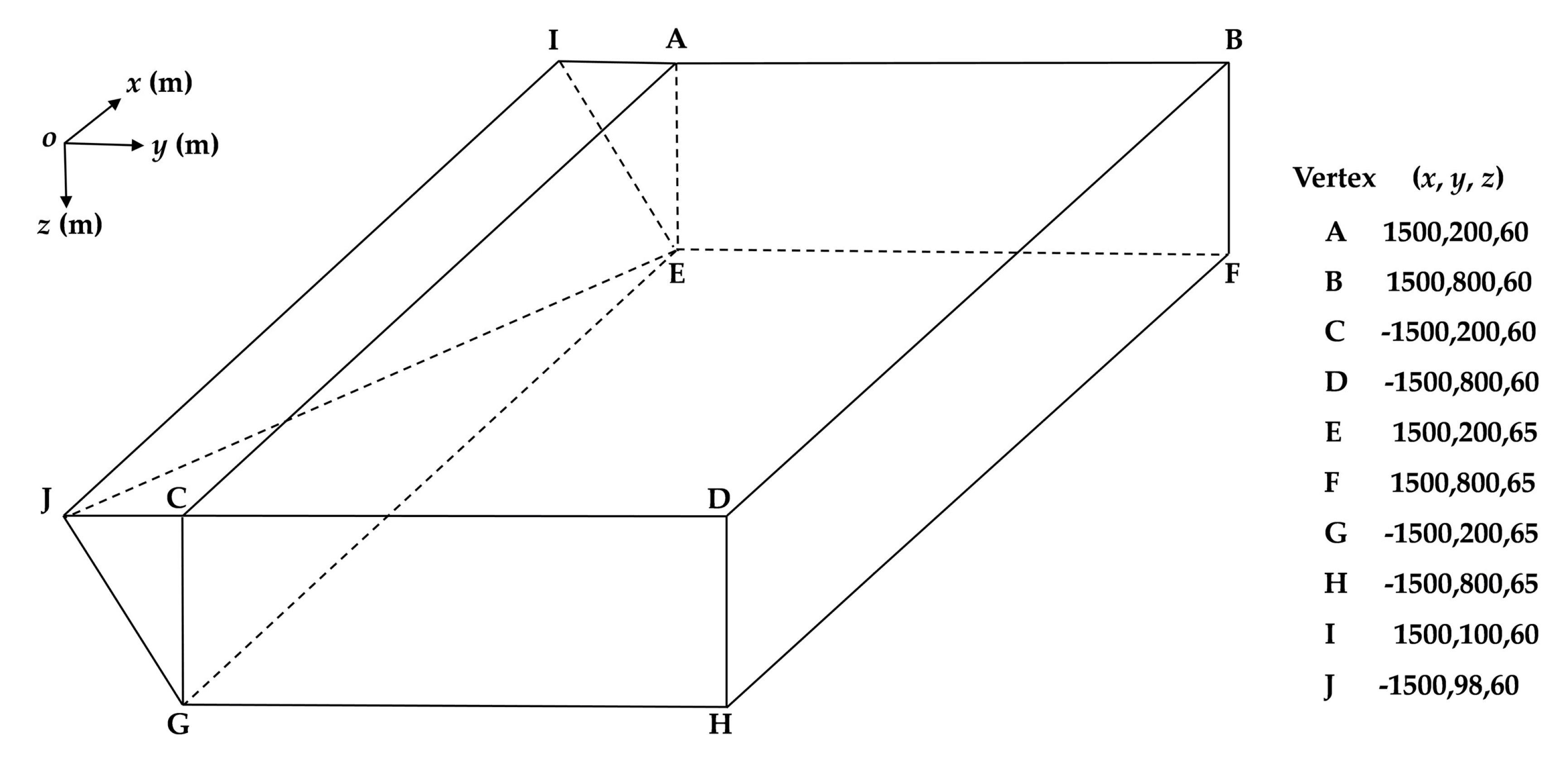
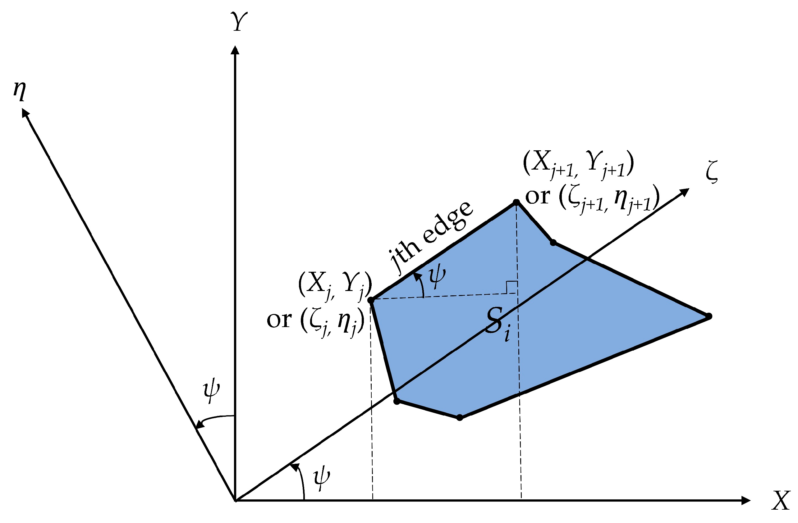
2.4. Principle of Gravitational Effect Computation

As discussed before, the layered polyhedron is the basic element for constructing the dynamic model of the water storage in the TGR. Previous studies [38,39] provided completely analytical expressions for the first and second derivatives of the gravitational potential in arbitrary directions generated by a homogeneous polyhedral body closed by polygonal facets.

Usually, the gravitational potential U, generated by a homogeneous body, can be given in integral form as

$$U(x,y,z)=G\rho {\displaystyle \underset{V}{\int }\frac{1}{r}dv}$$

(5)

where G is the constant of universal gravitation, ρ is the density of the body, V is the volume of the body, and r is the distance from origin point to integral element central point (x, y, z), i.e., r = (x² + y² + z²)^1/2.

The derivative of gravitational potential in arbitrary directions is the component of the attraction force in that direction. If U_k denotes the component of the attraction force in k-direction, it can be expressed as

$$U_k=\nabla U\cdot k=G\rho {\displaystyle \underset{V}{\int }\nabla \cdot \left(\frac{k}{r}\right)\hspace{0.17em}dv}$$

(6)

where the sign ∇ denotes gradient operator, k is the unit vector in k-direction. Applying the Gauss’s divergence theorem, Equation (6) becomes

$$U_k=G\rho {\displaystyle \underset{S}{\oint }\left(\frac{1}{r}\right)k\cdot \hspace{0.17em}nds}$$

(7)

where S is the closed surface of body V, n is the unit vector in outward normal direction on S. The S composes of finite number polygonal facets. Equation (7) can be rewritten in:

$$U_k=G\rho {\displaystyle \sum _{i}k\cdot \hspace{0.17em}{n}_i}{I}_i\hspace{0.17em},\hspace{1em}{I}_i={\displaystyle \underset{S_i}{\int }\frac{1}{r}d{s}_i}$$

(8)

where S_i is the ith facet, and n_i is the unit vector in outward normal direction on S_i.

For solving the surface integral in Equation (8), the coordinates may rotate to another Cartesian system (X, Y, Z), in which the Z-direction is coincident with n_i. The surface integral in the XOY plane is transformed to line integral along the closed edge of S_i based on the Green Formula. Because the edge composes of finite line-segments, line integral can be carried out by subsection integral. Hence, the surface integral of abbreviated expression is

$$I_i={\displaystyle \sum _j{J}_j(i)}$$

(9)

where J_j (i) indicates the line integral from jth vertex to (j + 1)th vertex on the edge of S_i. Vertexes must be numbered clockwise [39], and for the last edge, vertex (j + 1) corresponds to vertex 1. See Appendix A for detailed deducing process.

Finally, Equation (8) can be expressed as the summary of line integrals by following:

$$U_k=G\rho {\displaystyle \sum _i{\displaystyle \sum _{j}k\cdot \hspace{0.17em}{n}_i}}{J}_j(i)\hspace{0.17em}$$

(10)

The gravitational effect (g) usually represents the downward vertical component of the attraction force and the Equation (10) can be rewritten as

$$g=G\rho {\displaystyle \sum _i{\displaystyle \sum _j\cos {\varphi }_i}}{J}_j(i)\hspace{0.17em}$$

(11)

where ϕ_i is the spatial angle between the outward normal direction of S_i and downward vertical direction.

The Equation (11) is appropriate for computing the gravitational effects of the whole layered water body that includes the middle part of polygonal prism and polyhedron chains on the both banks, or only a single polyhedron. The gravitational effect of the water body at a certain water level can be obtained by accumulating those from the lowest water level.

Two simulating approaches are applied in this study. A synthetic model is designed and shown in Figure 8 in order to manifest the difference of the gravitational effects generated by water bodies. An asymmetry heptahedron (composed of a cuboid and an asymmetry hexahedron on the left, with regard to rough bank surface) is applied to simulate the model. The model density is defined as 1.0 × 10³ kg/m³ (i.e., fresh water). We selected observational points P₁(0,0,0), P₂(0,500,0), and P₃(0,1000,0), and the distance unit is meters. Afterwards, the gravitational effects at these points are calculated and listed in

Table 4. Experiment results from the complex body forward modeling method.

Simulating Approach	Gravitational Effect (μGal or 10−8 m/s2). at Observation Point
	P1	P2	P3
Cuboid	14.5003	181.7064	14.5003
Asymmetry heptahedron	21.3529	183.4860	14.7599
Asymmetry hexahedron (i.e., left part)	6.8526	1.7796	0.2596

. These results show that using the cuboid for simulation and without considering water on reservoir bank would result in loss of approximately 47% in gravitational effect near the riverside. Therefore, for comprehensive estimation of the gravitational effect, it is necessary to use polyhedrons to simulate water body instead of prism bodies.

3. Results

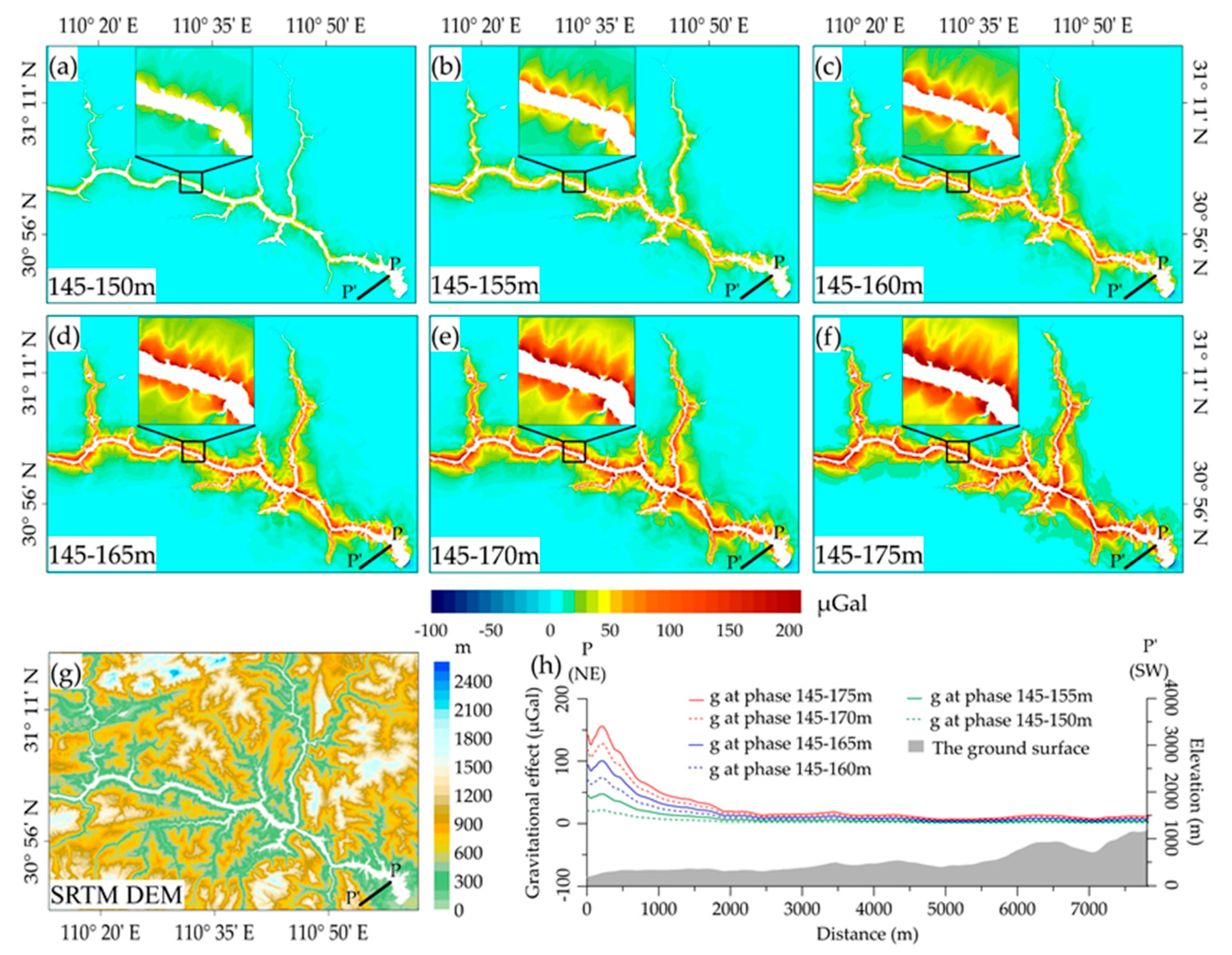
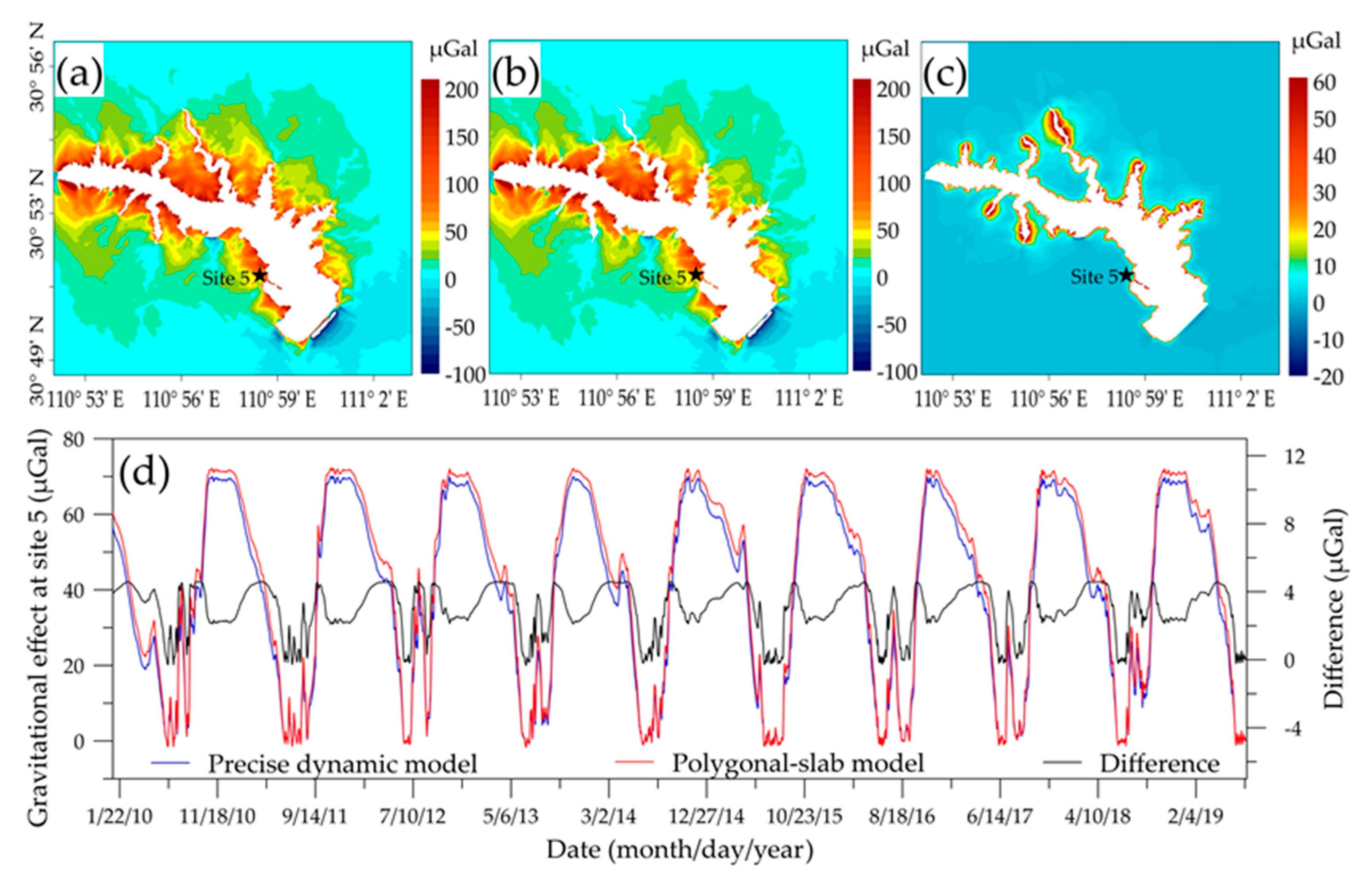
3.1. Gravitational Effects of Dynamic Water Storage in Head Region of TGR

Using the approach proposed in Section 2.4, we calculated the gravitational effects at different water impoundment periods based on the obtained water boundaries. In the theoretic modeling, the lowest and the highest water levels are defined at 145 m and 175 m, respectively. The gravitational effects on the surface in the head region of TGR are computed, for which SRTM DEM is employed to approximate the surface with a ground resolution of about 30 m.

Figure 9 shows results during six water impoundment periods. The gravitational effects increase with rising water levels, and the maximum of more than 600 μGal is obtained at period 145–175 m. Gravitational effects are negative at a few places because the elevation of observation points is lower than the water level at that place. There is a tendency for high gravitational effects to appear near the reservoir, and their intensity rapidly decays as distance from the reservoir bank increases. Furthermore, the impact of local water storage on gravitational effect is significantly increased in areas where tributaries meet. In general, the gravitational effects of water storage are affected by the relative distance of the local reservoir bank and the relative elevation difference between the calculation site and water level surface.

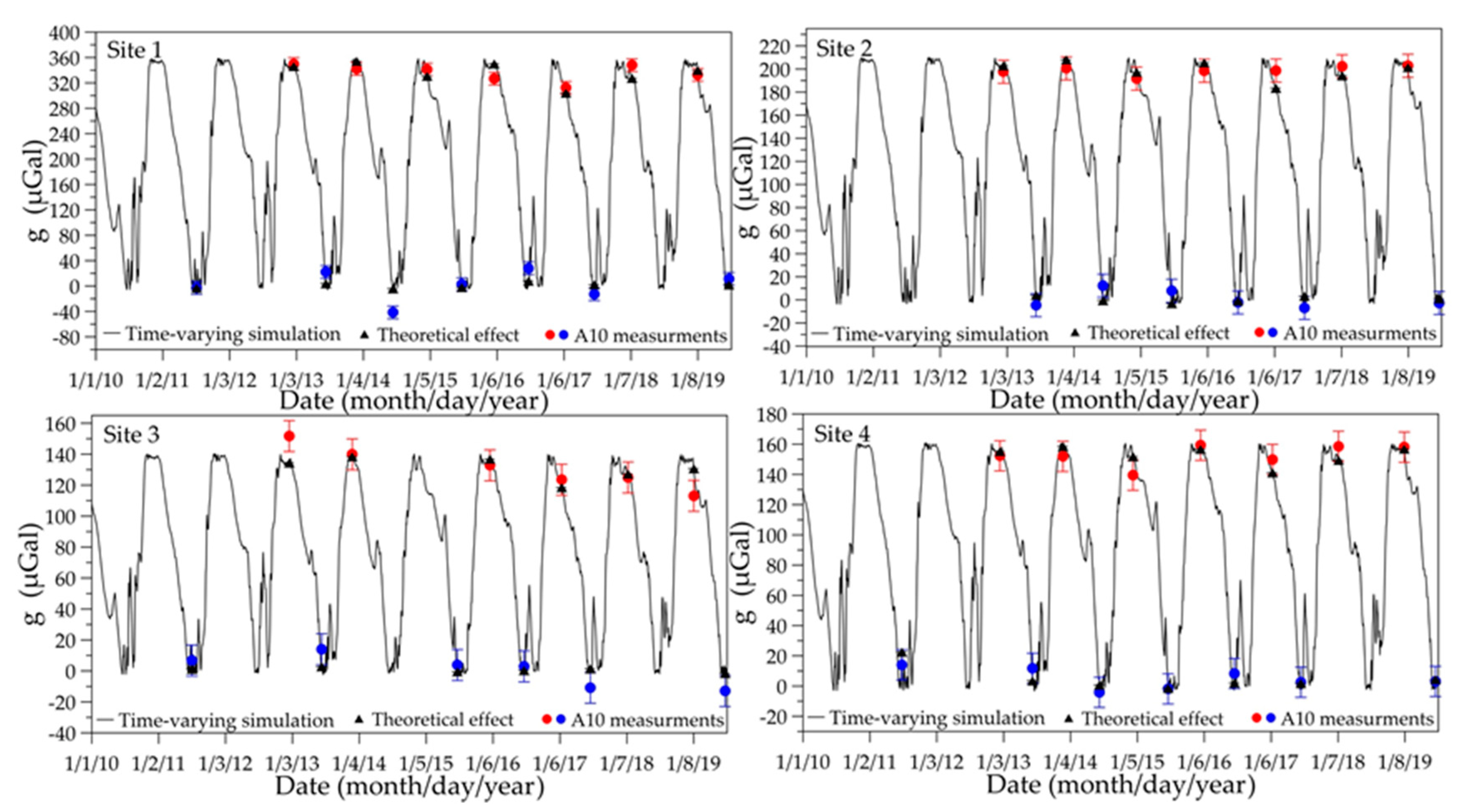
3.2. Comparison with the Measurement of Absolute Gravimeter

We selected four field gravity observation sites in the head region of TGR (Figure 5) that can be used for detecting regional gravity changes caused by impoundment. Afterwards, we calculated the time-varying gravitational effects based on dynamic water storage model at in situ observation sites (Figure 10). Since 2010, field observations of absolute gravity were carried out twice per year, i.e., in summer (low water level, ~145 m) and in winter (high water level, ~175 m). The field observations included vertical gravity gradient measurements from a drop cart position to the ground. This study used repeated measurements of absolute gravity to verify the validity and accuracy of forward modeling from the dynamic water storage model.

The results show that the A10 observations display a similarly regular cyclic gravitational effect due to periodical water storage changes controlled by the dam (Figure 10). Furthermore, the theoretical gravitational effects calculated by the dynamic water storage model are highly consistent with in situ measured A10 data. It should be noted that the measurements of A10 represent the absolute gravity values, while the calculated gravitational effect of the water body above the lowest water level is a relative value obtained by the dynamic water storage model. Thus, we have separately calculated the average values of the measured absolute gravity during the lowest and the highest water level impoundment period. For example, for the A10 observation data acquired during the lowest water level stage, we used the observed absolute gravity data (g_{observed in 145m}) minus the average value of all observed data (g_{observed mean in 145m}) during the lowest water level stage; then, we added the average value of the theoretical gravitational effects (g_{calculated mean in 145m}) in the corresponding observation time, as a comparison reference value of the measured data (i.e., g_{observed_lowest} = g_{observed in 145m} − g_{observed mean in 145m} + g_{calculated mean in 145m}). Afterwards, we used a similar process for the observation data acquired during the highest water level stage (i.e., g_{observed_highest} = g_{observed in 175m} − g_{observed mean in 175m} + g_{calculated mean in 175m}). The results show that the amplitude of gravitational effects varies greatly at different sites, which mainly depends on the mass changes and the relative position between A10 sites and the dynamic water storage model. The observed absolute gravity data verified the simulation predicted results with small deviations of a few to dozens of μGal. It has to be noted that the A10 observed results also include other potential environmental effects (e.g., climate-induced rainfall, groundwater storage variations, etc.), in addition to the direct gravitational effects of TGR impoundment and A10 instrument measurement uncertainty (10 μGal). These influencing factors will be discussed in the next section.

4. Discussion

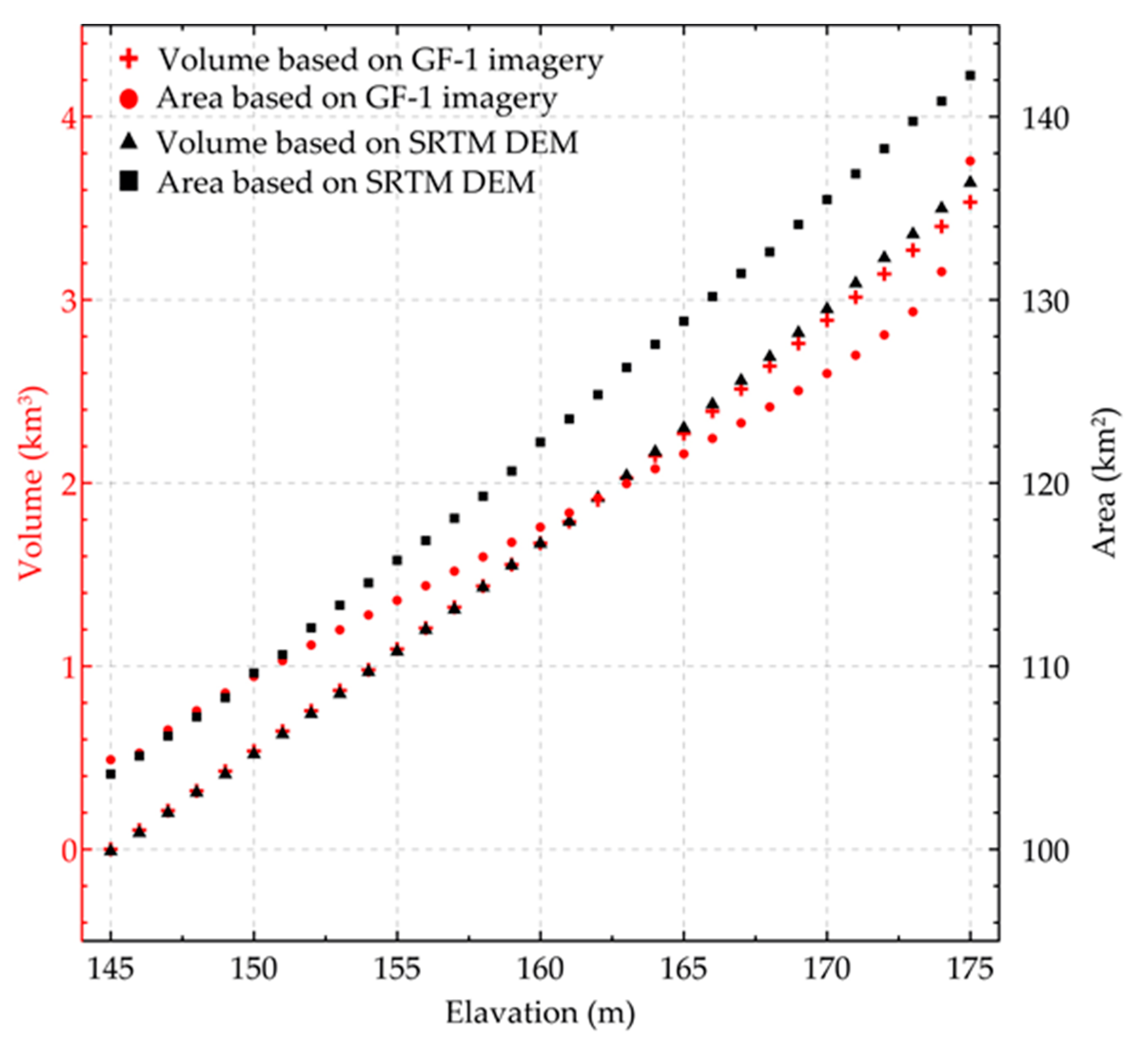
4.1. The Capacity of the Dynamic Water Storage Model

The dynamic water storage model constructed in the head region of TGR is mainly composed of the 31 water boundaries of the reservoir and the real-time water level in front of the dam. Accordingly, this model is based on the valid distribution pattern of the water body changes due to the artificially controlled dam. Compared with the previous static model constructed by SRTM DEM data (about 90 m resolution), our dynamic model is based on the GF-1 imagery that represents the changes of the water boundaries (more fit with the real water body) in different periods and with better resolution. For the variation of water storage in the head region of TGR, we calculated the volumes and inundated areas at different water levels by applying our dynamic water storage model and previous static model based on SRTM DEM (Figure 11).

The calculated volumes from two different water storage models are similar, yet the variation characteristics of inundated areas are different. The horizontal changes in riverbank lines basically vary on a few dozens of meters (Figure 5). Accordingly, the lower resolution of SRTM DEM (~90 m) in the previous static model can produce errors when recognizing river boundaries. This approximate result based on STRM may not show significant differences when we use the entire TGR hydrological information; however, it will show obvious impact in a small local area such as the head region of TGR. For example, if we assume that the water storage model adds 1 grid after the water level is increased by 1 m, then the increased area is mainly based on the horizontal resolution of the grid, i.e., the grid with 1-m resolution will cause an increase in the area of 1 m × 1 m, while a grid with a STRM 90-m resolution will result in an increase of 90 m × 90 m. For the local area selected in this study, our dynamic water storage model based on higher-resolution GF-1 data can provide more detailed river boundary changes.

4.2. Simulation Accuracy

The gravitational effect of a water storage model depends on the characteristics of the model itself and the spatial position between the observation site and the model, i.e., the difference in distance and height between the calculation point and the model. In this study, we tested the impacts of the forward modeling accuracy due to different resolution of model boundary. Firstly, we applied a dynamic polygonal-slab model that only uses the lowest and the highest water boundaries as the model boundary. This simplified slab model can approximate slope surface to vertical plane when calculating the gravitational effect, yet it neglects the influence of the millions of triangular facets of the slope (see Figure 7d). Afterwards, we calculated and compared the gravitational effects in the surrounding region based on the dynamic polygonal-slab model (Figure 12a) and the precise dynamic water storage model (Figure 12b). The comparison results show that the dynamic polygonal-slab model will cause a large calculation error when the water boundary near the reservoir bank drastically changes (Figure 12c). In other words, when the area is closer to the water body, there is also larger amplitude in gravitational effect changes and the calculation error in simplified models. This is especially evident in the tributary area where the calculation error changes faster. The dynamic polygonal-slab model is characterized by the fast calculation speed and is suitable for the analysis of the distant area from the river bank (e.g., distance over 2000 m), where the amplitude of gravitational effect of the water storage model is relatively small and slowly fluctuates (Figure 9h).

For the situation at the single observation site (e.g., site 5 in Figure 5), we calculated the time-varying gravitational effects based on the precise dynamic water storage model and the dynamic polygonal-slab model, respectively (Figure 12d). The distance of horizontal position and elevation difference between site 5 and the nearest model boundary (Figure 5) are ~349 m and ~93 m (relative to 145 m), respectively. The maximum variation amplitude of the theoretical gravitational effect at site 5 can reach up to 70 μGal based on the dynamic water storage model, and the maximum difference can reach up to 4.58 μGal. It is noticed that the difference between the two water storage models will be larger when the observation site or the calculation point is closer to the river bank. Moreover, gravitational effects based on two water model appear to be significantly inconsistent with different water levels, e.g., the difference between the forward modeling results of the two models is relatively large during sharp fluctuations of water level (releasing water in spring and flooding in monsoon) and relatively small during stable water level periods. In this case, the precise dynamic water storage model can identify with greater accuracy the local boundary changes and is more suitable for precise correction of observational points around the reservoir banks in order to extract other hydrological or geophysical signals, e.g., groundwater leakage and tectonic movement.

4.3. Other Influences

We noticed that our model simulation results are in good agreement with the gravity observational data at larger gravity difference scales (e.g., dozens or even hundreds of μGal as shown in Figure 10). This indicates that the change in gravitational effects caused by the impoundment is the main factor for the non-tidal gravity changes within 1000 m of the reservoir bank, with a few subtle differences between modelled and observed results. In fact, A10 absolute gravity observations reflect all gravity effects including TGR water impoundment and other surface processes around the site, after performed preprocessing (e.g., removal of effects such as solid earth tides, ocean tides, pole motion, normal field, and elevation correction at each site). For example, several unknown environmental gravity changes such as groundwater changes [5], seasonal changes in rainfall [4], and tectonic movements [13] are reflected in A10 results, and they can cause gravity changes of about 10 μGal [28]. Wang et al. [5] showed that the interannual change of the equivalent groundwater height in the TGR area is about 1.6 m, which leads to the observed gravitational changes of up to tens of μGal.

The elastic deformation of the Earth caused by the huge impoundment water load can also cause the change of the gravitational field [12], yet its amplitude is relatively small (within 6 μGal). In addition, regional economic development (e.g., construction of roads, bridges, buildings, etc.) and local topographic changes caused by geological disasters like landslides are also factors that can cause disagreement between simulated and measured results. Overall, these factors should be considered in future study, e.g., by separating secondary signals directly or indirectly from the water storage changes in TGR.

5. Conclusions

In this study, we used GF-1 high-resolution satellite imageries and water level in front of the dam in order to develop a dynamic water storage model which would provide support for the fine simulation of the surface dynamics of TGR. By utilizing the forward modeling method of complex body, it was possible to obtain the high-precision simulation results of gravitational effects that provide important real-time hydrologic correction data for identifying and distinguishing the gravitational effects between TGR-induced water changes and other hydrological elements. The main conclusions are as follows:

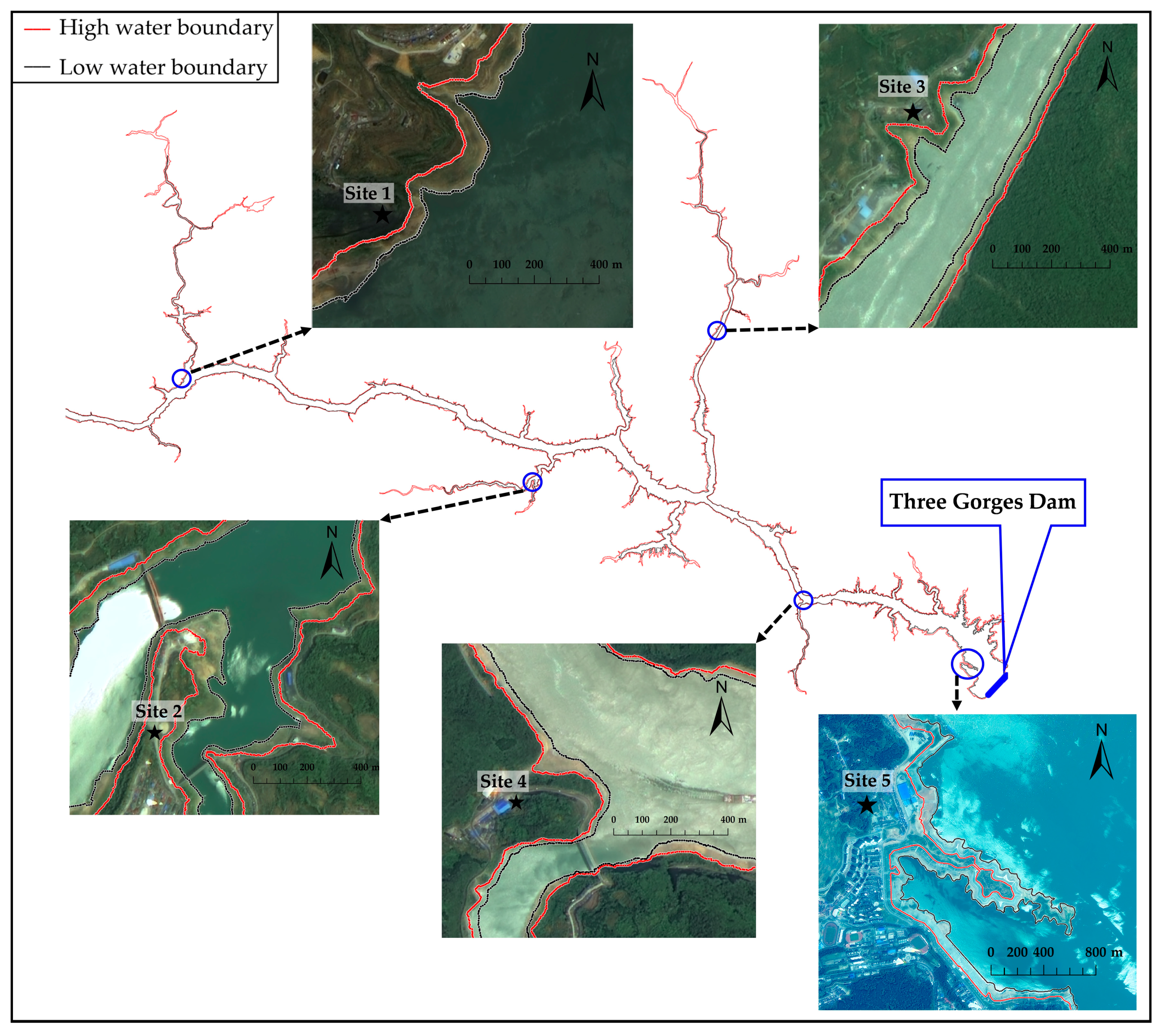
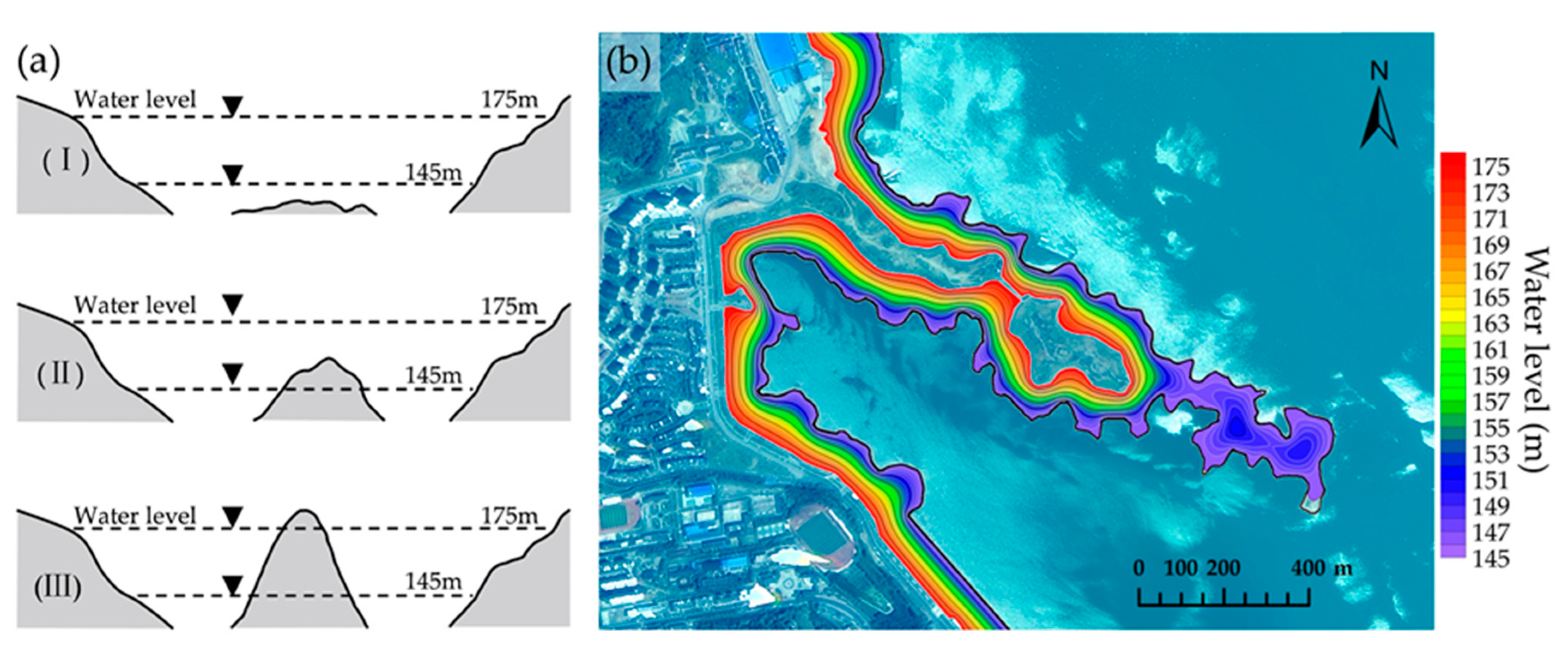
• In front of the dam (Zigui area), the annual water boundary change can be up to 100 m in horizontal direction. In the tributary area of the TGR, the changes of the water boundary are more obvious, especially in the north of Badong area. The dynamic water storage model constructed in this study consists of water boundaries (31 in total) at different impoundment periods, i.e., from 145 m to 175 m. The resolution of the model is approximately 8 m in horizontal direction and approximately 1 m in vertical direction, which is an important way to describe the local dynamic characteristics in the impounding and releasing water process.
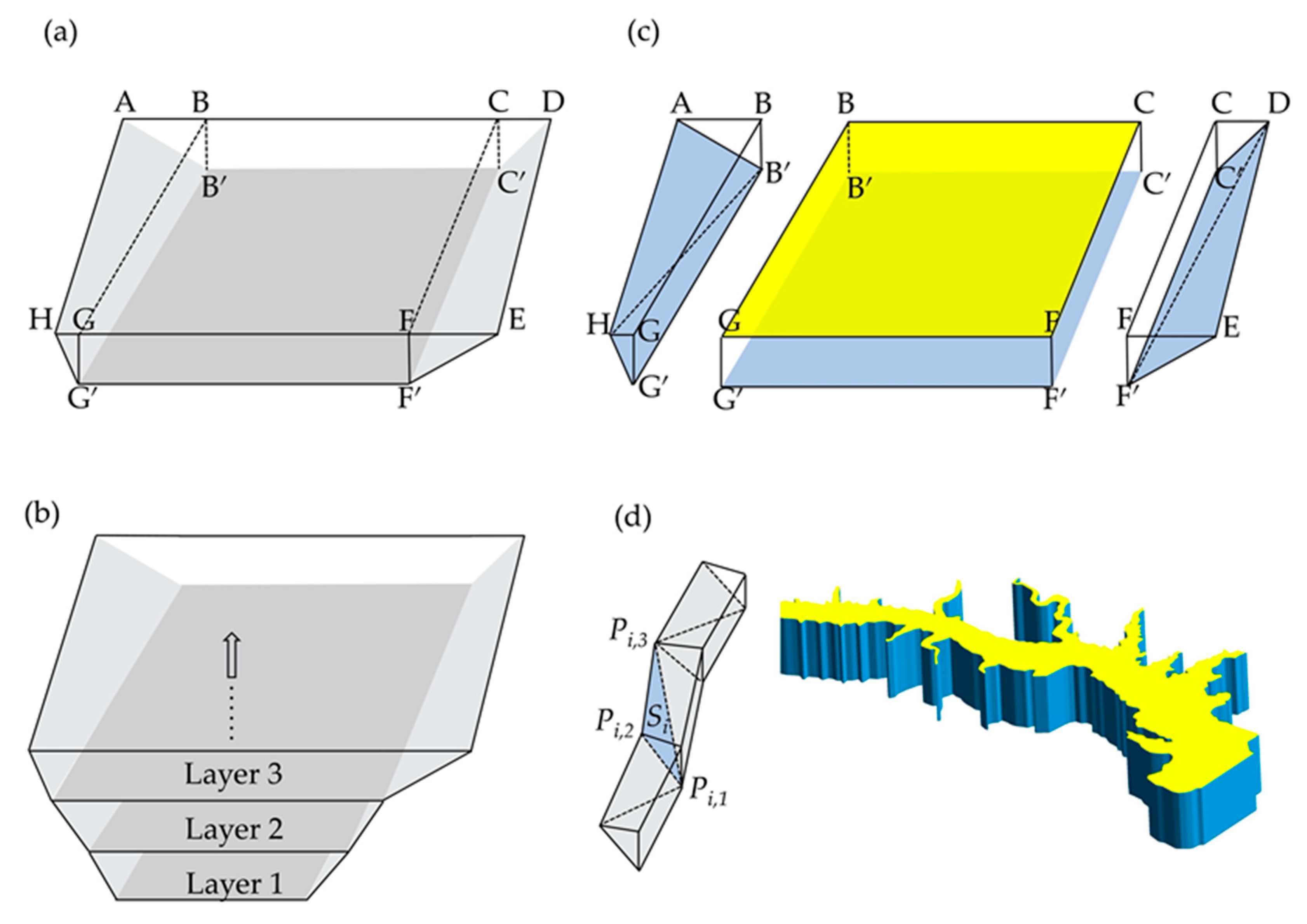
• The high-precision forward modeling method of gravitational effect can avoid the error caused by model approximation. The gravitational effect of TGR water storage is obvious within 1000 m of the reservoir bank, and the maximum gravity change caused by the 30-m water level change (from 145 m to 175 m) can reach nearly 600 μGal. The ground multiyear gravity observation data from A10 absolute gravimeters verified the simulations. Our results confirm that the gravitational effects change caused by TGR impoundment is the main contribution of the gravity field changes in the study area. The differences between in situ observations and simulation results can help in further tracking of the effects of geological disasters, such as earthquakes and landslides.
• The comparison results show that the dynamic water storage model has more advantages in identifying changes in water storage in local areas and is statistically more accurate in obtaining TGR capacity information when compared to the previous model. However, the potential users should consider the spatial position and coordinate accuracy of the calculated point when applying the dynamic water storage model.
• The accuracy of the dynamic water storage model is related to factors such as satellite imagery preprocessing (e.g., data calibration), imagery quality, cloud cover, and extraction method for water boundaries. In addition, manual visual interpretation can solve the influence of interference factors (e.g., river vessels, mountain shadows, water pollutants, etc.) With the continuous accumulation and update of the remote sensing data and the development of water boundary extraction technology, it can be expected that the accuracy of the water storage model will be improved in the future.

References

1. Wang, J.; Sheng, Y.; Gleason, C.J.; Wada, Y. Downstream Yangtze River levels impacted by Three Gorges Dam. Environ. Res. Lett. 2013, 8, 044012. [Google Scholar] [CrossRef]
2. Long, D.; Yang, Y.; Wada, Y.; Hong, Y.; Liang, W.; Yaning, C.; Yong, B.; Hou, A.; Wei, J.; Chen, L. Deriving scaling factors using a global hydrological model to restore GRACE total water storage changes for China’s Yangtze River Basin. Remote Sens. Environ. 2015, 168, 177–193. [Google Scholar] [CrossRef]
3. Boy, J.P.; Chao, B.F. Time-variable gravity signal during the water impoundment of China’s Three-Gorges Reservoir. Geophys. Res. Lett. 2002, 29, 2200. [Google Scholar] [CrossRef] [Green Version]
4. Wang, X.W.; Linage, C.; Famiglietti, J.; Zender, C.S. Gravity Recovery and Climate Experiment (GRACE) detection of water storage changes in the Three Gorges Reservoir of China and comparison with in situ measurements. Water Resour. Res. 2011, 47, W12502. [Google Scholar] [CrossRef]
5. Wang, W.; Zhang, C.Y.; Liang, S.M.; Yang, Q.; Hu, M.Z.; Feng, W. Monitoring of the temporal and spatial variation of groundwater storage in the Three Gorges area based on the CORS network. J. Appl. Geophys. 2017, 146, 160–166. [Google Scholar] [CrossRef]
6. Li, F.P.; Wang, Z.T.; Chao, N.F.; Song, Q.Y. Assessing the Influence of the Three Gorges Dam on Hydrological Drought Using GRACE Data. Water. 2018, 10, 669. [Google Scholar] [CrossRef] [Green Version]
7. Tang, H.M.; Wasowski, J.; Juang, C.H. Geohazards in the three Gorges Reservoir Area, China–Lessons learned from decades of research. Eng. Geol. 2019, 261, 105267. [Google Scholar] [CrossRef]
8. Wang, W.; Zhang, C.Y.; Hu, M.Z.; Yang, Q.; Liang, S.M.; Kang, S.J. Monitoring and analysis of geological hazards in Three Gorges area based on load impact change. Nat. Hazards 2019, 97, 611–622. [Google Scholar] [CrossRef]
9. Wang, Y.; Liao, M.; Sun, G.; Gong, J. Analysis of the water volume, length, total area and inundated area of the Three Gorges Reservoir, China using the SRTM DEM data. Int. J. Remote Sens. 2005, 26, 4001–4012. [Google Scholar] [CrossRef]
10. Wang, X.W.; Chen, Y.; Song, L.C.; Chen, X.Y.; Xie, H.J.; Liu, L. Analysis of lengths, water areas and volumes of the Three Gorges Reservoir at different water levels using Landsat images and SRTM DEM data. Quat. Int. 2013, 304, 115–125. [Google Scholar] [CrossRef]
11. Wang, L.S.; Chen, C.; Zou, R.; Du, J.S. Surface gravity and deformation effects of water storage changes in China’s Three Gorges Reservoir constrained by modeled results and in situ measurements. J. Appl. Geophys. 2014, 108, 25–34. [Google Scholar] [CrossRef]
12. Wang, L.S.; Chen, C.; Ma, X.; Du, J.S. A Water Storage Loading Model by SRTM-DEM Data and Surface Response Simulation of Gravity and Deformation in the Three Gorges Reservoir of China. Acta Geod. Cartogr. Sin. 2016, 45, 1148–1156, (In Chinese with English Abstract). [Google Scholar] [CrossRef]
13. Yao, Y.S.; Wang, Q.L.; Liao, W.L.; Zhang, L.F.; Chen, J.H.; Li, J.G.; Yuan, L.; Zhao, Y.N. Influences of the Three Gorges Project on seismic activities in the reservoir area. Sci. Bull. 2017, 62, 1089–1098. [Google Scholar] [CrossRef] [Green Version]
14. Zhang, L.; Yang, D.X.; Liu, Y.W.; Che, Y.T.; Qin, D.J. Impact of impoundment on groundwater seepage in the Three Gorges Dam in China based on CFCs and stable isotopes. Environ. Earth Sci. 2014, 72, 4491–4500. [Google Scholar] [CrossRef]
15. Farr, T.G.; Rosen, P.A.; Caro, E.; Crippen, R.; Duren, R.; Hensley, S.; Kobrick, M.; Paller, M.; Rodriguez, E.; Roth, L.; et al. The Shuttle Radar Topography Mission. Rev. Geophys. 2007, 45, RG2004. [Google Scholar] [CrossRef] [Green Version]
16. Rodriguez, E.; Morris, C.S.; Belz, J.E. A global assessment of the SRTM performance. Photogramm. Eng. Remote Sens. 2006, 72, 249–260. [Google Scholar] [CrossRef] [Green Version]
17. Zhang, G.Q.; Yao, T.D.; Chen, W.F.; Zheng, G.X.; Shum, C.K.; Yang, K.; Piao, S.L.; Sheng, Y.W.; Yi, S.; Li, J.L.; et al. Regional differences of lake evolution across China during 1960s–2015 and its natural and anthropogenic causes. Remote Sens. Environ. 2019, 221, 386–404. [Google Scholar] [CrossRef]
18. Wang, M.L.; Du, L.J.; Ke, Y.H.; Huang, M.Y.; Zhang, J.; Zhao, Y.; Li, X.J.; Gong, H.L. Impact of Climate Variabilities and Human Activities on Surface Water Extents in Reservoirs of Yong ding River Basin, China, from 1985 to 2016 Based on Landsat Observations and Time Series Analysis. Remote Sens. 2019, 11, 560. [Google Scholar] [CrossRef] [Green Version]
19. Entwistle, N.; Heritage, G.; Milan, D. Recent remote sensing applications for hydro and morpho dynamic monitoring and modelling. Earth Surf. Process. Landf. 2018, 43, 2283–2291. [Google Scholar] [CrossRef]
20. Wang, C.; Jia, M.M.; Chen, N.C.; Wang, W. Long-Term Surface Water Dynamics Analysis Based on Landsat Imagery and the Google Earth Engine Platform: A Case Study in the Middle Yangtze River Basin. Remote Sens. 2018, 10, 1635. [Google Scholar] [CrossRef] [Green Version]
21. Rokni, K.; Ahmad, A.; Selamat, A.; Hazini, S. Water Feature Extraction and Change Detection Using Multitemporal Landsat Imagery. Remote Sens. 2014, 6, 4173–4189. [Google Scholar] [CrossRef] [Green Version]
22. Zhang, G.Q.; Zheng, G.X.; Gao, Y.; Xiang, Y.; Lei, Y.B.; Li, J.L. Automated Water Classification in the Tibetan Plateau Using Chinese GF-1 WFV Data. Photogramm. Eng. Remote Sens. 2017, 83, 509–519. [Google Scholar] [CrossRef]
23. Zhang, Z.Y.; He, H.X.; Yu, C.H.; Zhang, W.; Li, L.Y.; Meng, L.K. Using the modified two-mode method to identify surface water in Gaofen-1 images. J. Appl. Remote Sens. 2018, 13, 022003. [Google Scholar] [CrossRef]
24. Du, W.Y.; Chen, N.C.; Liu, D.N. Automatic Balloon Snake Method for Topology Adaptive Water Boundary Extraction: Using GF-1 Satellite Imagery as an Example. IEEE J. Sel. Top. Appl. Earth Observ. Remote Sens. 2017, 10, 5381–5394. [Google Scholar] [CrossRef]
25. Du, W.Y.; Chen, N.C.; Liu, D.N. Topology adaptive water boundary extraction based on a modified balloon snake: Using GF-1 satellite images as an example. Remote Sens. 2017, 9, 140. [Google Scholar] [CrossRef] [Green Version]
26. Zhu, S.Y.; Wan, W.; Xie, H.J.; Liu, B.J.; Li, H.; Hong, Y. An efficient and effective approach for georeferencing AVHRR and GaoFen-1 imageries using inland water bodies. IEEE J. Sel. Top. Appl. Earth Observ. Remote Sens. 2018, 11, 2491–2500. [Google Scholar] [CrossRef]
27. David, C.; Caroline, D.L.; Jacques, H.; Boy, J.P.; Famiglietti, J. A comparison of the gravity field over Central Europe from superconducting gravimeters, GRACE and global hydrological models, using EOF analysis. Geophys. J. Int. 2012, 189, 877–897. [Google Scholar] [CrossRef] [Green Version]
28. Crossley, D.; Hinderer, J.; Riccardi, U. The measurement of surface gravity. Rep. Prog. Phys. 2013, 76, 046101. [Google Scholar] [CrossRef]
29. Wang, H.; Hsu, H.T.; Zhu, Y.Z. Prediction of surface horizontal displacements, and gravity and tilt changes caused by filling the Three Gorges Reservoir. J. Geod. 2002, 76, 105–114. [Google Scholar] [CrossRef]
30. McFeeters, S.K. The use of the Normalized Difference Water Index (NDWI) in the delineation of open water features. Int. J. Remote Sens. 1996, 17, 1425–1432. [Google Scholar] [CrossRef]
31. McFeeters, S.K. Using the normalized difference water index (NDWI) within a geographic information system to detect swimming pools for mosquito abatement: A practical approach. Remote Sens. 2013, 5, 3544–3561. [Google Scholar] [CrossRef] [Green Version]
32. Ji, L.; Zhang, L.; Wylie, B. Analysis of dynamic thresholds for the normalized difference water index. Photogramm. Eng. Remote Sens. 2009, 75, 1307–1317. [Google Scholar] [CrossRef]
33. Feyisa, G.L.; Meilby, H.; Fensholt, R.; Rroud, S.R. Automated Water Extraction Index: A new technique for surface water mapping using Landsat imagery. Remote Sens. Environ. 2014, 140, 23–35. [Google Scholar] [CrossRef]
34. Otsu, N. A threshold selection method from gray-level histograms. IEEE Trans. Syst. Man Cybern. 1979, 9, 62–66. [Google Scholar] [CrossRef] [Green Version]
35. Ma, R.F.; Duan, H.T.; Hu, C.M.; Feng, X.Z.; Li, A.N.; Ju, W.M.; Jiang, J.H.; Yang, G.S. A half-century of changes in China’s lakes: Global warming or human influence? Geophys. Res. Lett. 2010, 37, L24106. [Google Scholar] [CrossRef]
36. Ma, R.F.; Yang, G.S.; Duan, H.T.; Jiang, J.H.; Wang, S.M.; Feng, X.Z.; Li, A.N.; Kong, F.X.; Xue, B.; Wu, J.L.; et al. China’s lakes at present: Number, area and spatial distribution. Sci. China Earth Sci. 2011, 54, 283–289. [Google Scholar] [CrossRef]
37. Wan, W.; Long, D.; Hong, Y.; Ma, Y.Z.; Yuan, Y.; Xiao, P.F.; Duan, H.T.; Han, Z.Y.; Gu, X.F. A lake data set for the Tibetan Plateau from the 1960s, 2005, and 2014. Sci. Data 2016, 3, 160039. [Google Scholar] [CrossRef] [Green Version]
38. Barnett, C.T. Theoretical modeling of the magnetic and gravitational fields of an arbitrary shaped three-dimensional body. Geophysics 1976, 41, 1353–1364. [Google Scholar] [CrossRef]
39. Okabe, M. Analytical expressions for gravity anomalies due to homogeneous polyhedral bodies and translations into magnetic anomalies. Geophysics 1979, 44, 730–741. [Google Scholar] [CrossRef]
Publisher’s Note: MDPI stays neutral with regard to jurisdictional claims in published maps and institutional affiliations.
Figure 1. The location of study area. The topography data is DEM from the Shuttle Radar Topography Mission (SRTM v3, https://lpdaac.usgs.gov/products/srtmgl1v003/).
Remotesensing 12 03353 g001
Figure 2. Flowchart of GF-1 Panchromatic and Multispectral Scanners (PMS) data preprocessing.
Remotesensing 12 03353 g002
Figure 3. Procedure of water boundary extraction.
Remotesensing 12 03353 g003
Figure 4. Example of water boundary extraction. (a) Preprocessed GF-1 imagery; (b) Normalized Differential Water Index (NDWI) imagery from (a); (c) tracked water boundaries overlapped (a); (d) the corrected water boundaries by manual visual interpretation.
Remotesensing 12 03353 g004
Figure 5. Schematic view of extracted water boundary lines at water levels at about 145 m (black dotted line) and 175 m (red dotted line) and spatial distribution of A10 absolute gravity observation sites in the head region of TGR. The base map is the imagery when the water level is at about 145 m.
Remotesensing 12 03353 g005
Figure 6. (a) Sketch of river channel sections for different underwater topography features in the TGR area with three types of situations: (I), (II), and (III); (b) Extracted and interpolated water boundaries at different water levels in the part of GF-1 imagery (ID: 2446123).
Remotesensing 12 03353 g006
Figure 7. Sketches of a segment of river water volume: (a) one layer water body; AH and DE are the segments of water boundary lines on two riversides on the higher water level; B′G′ and C′F′ are those on the lower water level; (b) combined multi-layers of water body; (c) separated (a) with the middle representing a quadrilateral prism, and the bodies on two sides are two pentahedrons, with ABG′H′ and C′DRF′ representing two surface facets on immerged riverbank; (d) 3D views of connected adjacent polyhedrons along a reservoir bank and the polygonal-slab composed of numerous segment quadrilateral prisms in one layer.
Remotesensing 12 03353 g007
Figure 8. A synthetic model shaped as an asymmetric heptahedron with a density of 1.0 × 10³ kg/m3. Two horizontal planar facets on the top and bottom of the model represent the water levels. The dip rectangular facet IJGE represents the assumptive bank surface facet. This body may be considered as a union combined by a cuboid and an asymmetry hexahedron according to the vertex setting. The bank surface can be represented by two triangular facets ΔIEJ and ΔJEG.
Remotesensing 12 03353 g008
Figure 9. The theoretic gravitational effects in the head region of TGR during six impoundment periods. Data is computed on the surface in a grid of 30 m × 30 m, except for the water area, by using the highest water level boundary. Panels (af) show gravitational effects at impoundment periods of 145–150 m, 145–155 m, 145–160 m, 145–165 m, 145–170 m, and 145–175 m, respectively; (g) shows the DEM of the area; (h) shows the gravitational effects of all periods on the profile PP.
Remotesensing 12 03353 g009
Figure 10. Time-varying simulation of gravitational effects at four observation sites and the actual observed absolute gravity results. The blue dots represent A10 observed results during the lowest water level period and the red dots represent A10 observed results during the highest water level period, while the error bars represent the uncertainty of A10 observations. The black triangles represent the theoretical gravitational effect when A10 measurements were carried out.
Remotesensing 12 03353 g010
Figure 11. Mathematical fitting relationship of water volume, inundated area, and water level values in the head region of TGR based on the water storage models obtained from GF-1 imagery and SRTM DEM.
Remotesensing 12 03353 g011
Figure 12. Regional gravitational effects of impoundment water body (145 m–175 m) using different models, in the head region of dam. (a) Polygonal-slab model; (b) precise dynamic model; (c) difference between (a) and (b); (d) time-varying simulation of gravitational effects at site 5 based on precise dynamic model (blue line) and dynamic polygonal-slab model (red line), and its difference (black line).
Remotesensing 12 03353 g012