Article

Capturing the Impact of the 2018 European Drought and Heat across Different Vegetation Types Using OCO-2 Solar-Induced Fluorescence

1
TUM Department of Electrical and Computer Engineering, Technical University of Munich, 80333 Munich, Germany
2
Department of Environmental Systems Science, ETH Zurich, 8092 Zurich, Switzerland
3
TUM School of Life Science Weihenstephan, Technical University of Munich, 85354 Freising, Germany
*
Author to whom correspondence should be addressed.
Remote Sens. 2020, 12(19), 3249; https://doi.org/10.3390/rs12193249
Submission received: 11 August 2020 / Revised: 20 September 2020 / Accepted: 30 September 2020 / Published: 6 October 2020
(This article belongs to the Special Issue Drought Monitoring Using Satellite Remote Sensing)

Abstract

:
The European heatwave of 2018 led to record-breaking temperatures and extremely dry conditions in many parts of the continent, resulting in widespread decrease in agricultural yield, early tree-leaf senescence, and increase in forest fires in Northern Europe. Our study aims to capture the impact of the 2018 European heatwave on the terrestrial ecosystem through the lens of a high-resolution solar-induced fluorescence (SIF) data acquired from the Orbiting Carbon Observatory-2 (OCO-2) satellite. SIF is proposed to be a direct proxy for gross primary productivity (GPP) and thus can be used to draw inferences about changes in photosynthetic activity in vegetation due to extreme events. We explore spatial and temporal SIF variation and anomaly in the spring and summer months across different vegetation types (agriculture, broadleaved forest, coniferous forest, and mixed forest) during the European heatwave of 2018 and compare it to non-drought conditions (most of Southern Europe). About one-third of Europe’s land area experienced a consecutive spring and summer drought in 2018. Comparing 2018 to mean conditions (i.e., those in 2015–2017), we found a change in the intra-spring season SIF dynamics for all vegetation types, with lower SIF during the start of spring, followed by an increase in fluorescence from mid-April. Summer, however, showed a significant decrease in SIF. Our results show that particularly agricultural areas were severely affected by the hotter drought of 2018. Furthermore, the intense heat wave in Central Europe showed about a 31% decrease in SIF values during July and August as compared to the mean over the previous three years. Furthermore, our MODIS (Moderate Resolution Imaging Spectroradiometer) and OCO-2 comparative results indicate that especially for coniferous and mixed forests, OCO-2 SIF has a quicker response and a possible higher sensitivity to drought in comparison to MODIS’s fPAR (fraction of absorbed photosynthetically active radiation) and the Normalized Difference Vegetation Index (NDVI) when considering shorter reference periods, which highlights the added value of remotely sensed solar-induced fluorescence for studying the impact of drought on vegetation.

Graphical Abstract

1. Introduction

Anthropogenic global warming is estimated to currently have reached about 1 °C above preindustrial levels and is estimated to further increase to 1.5 °C between 2030 and 2052 under current rates of greenhouse gas (GHG) emissions [1]. This increase in global temperature is expected to lead to an increase in intensity and frequency of extreme events such as heatwaves, drought, and associated wildfires [2,3,4]. In 2018, Europe faced such an extreme event characterized by record-breaking temperatures and long-lasting dryness, referred to as “hotter drought” [5]. According to the European Drought Observatory of the European Commission, most of Northern and Central Europe was affected by such hotter drought in 2018. On the contrary, much of the Southern Mediterranean Europe experienced relatively cool and moist conditions [6,7]. For Central Europe, various news and media articles reported severe decrease in crop yields, increase in elderly mortality, and forest fires along with many other adverse impacts. According to a quick attribution study by the World Weather Attribution on the heat in Northern Europe [8], the anthropogenic climate change has more than doubled the probability of occurrence of such a heatwave in the region.
Along with severe economic implications and adverse health impact on the public, such record-breaking hotter drought events severely affect ecosystems. A direct comparison of vegetation response to the drought in 2018 and the 2003 European heatwaves using MODIS’s vegetation indices concluded that negative impacts in 2018 were even stronger than in 2003, with a strong decline in agricultural land and forests, especially in Central Europe [6]. Such drought events strongly affect the carbon cycle by leading to plant mortality and reductions in ecosystem carbon dioxide (CO2) uptake, with the potential to convert ecosystems from carbon sinks into carbon sources [9,10].
Gross primary productivity (GPP) is a measure of ecosystem CO2 assimilation. The estimation and modeling of regional or global GPP involves various uncertainties arising from model parameterization [11,12], thus demanding a more direct and reliable approach to estimate GPP. With recent advances in satellite-based measurements of solar-induced (chlorophyll) fluorescence (SIF), it is now possible to use SIF as a direct proxy for photosynthesis or GPP worldwide [13,14,15,16,17]. SIF is an electromagnetic signal emitted in the wavelength range of 600 to 800 nm by chlorophyll molecules [18]. Since SIF is directly associated with photosynthesis, it is more physiologically-based compared to the traditionally used vegetation indices (VIs), such as the Normalized Difference Vegetation Index (NDVI) and the Enhanced Vegetation Index (EVI) [19,20]. Over the last decade, several studies have demonstrated a strong linear relationship between satellite-based SIF and GPP [13,15,21,22,23,24,25,26,27,28], indicating that SIF might provide a useful approximation of GPP. The SIF retrievals obtained from the Japanese Greenhouse Gases Observing Satellite (GOSAT) and the European Global Ozone Monitoring Experiment-2 (GOME-2) were most widely used in the last decade (2007–2017; see studies in [21,22,23,24,28]). However, due to coarse spatial resolution of the SIF footprint (10 km diameter for GOSAT and 40 × 40 km2 for GOME-2), these satellites presently impose serious limitations in detecting ecophysiological changes across different vegetation types. The recent NASA’s Orbiting Carbon Observatory-2 (OCO-2) satellite (launched in September 2014) provides SIF data at a much higher spatial resolution of 1.3 × 2.25 km2 with increased SIF acquisition frequency, thereby allowing us to resolve SIF responses of various vegetation types under different climatic conditions [15,29].
SIF acquired from GOSAT and GOME-2 have been previously used to study the effect of drought on vegetation. Using GOSAT’s SIF [30] showed that midday fluorescence explained the water stress over the Amazonian forests during a dry season in 2010. Yoshida et al. [31] used GOME-2′s SIF to study the impact of the 2010 Russian drought, and they highlighted the drought-related SIF decrease for croplands and grasslands. Sun et al. [32] studied the drought onset mechanisms and its impact on agriculture using GOME-2 SIF during the drought of 2011 in Texas and that of 2012 in the central Great Plains, United States. They concluded that SIF is sensitive to both structural and physiological variation in vegetation during drought and considered it an appropriate tool for drought monitoring. Koren et al. [33] developed a GOME-2 based SIF product to show that spatial SIF response was in good agreement with meteorological (temperature, soil moisture, evapotranspiration, and terrestrial water storage) anomalies during the 2015–2016 El Niño Amazon drought. Recently, Zhang et al. [34] constructed a global gridded SIF dataset (CSIF) using a neural network trained by OCO-2 and MODIS data, which they also employed for drought monitoring. Their preliminary result showed that the CSIF well captured the spatial extent of droughts during the 2015 European heatwave.
Here, we present the impact of the 2018 European hotter drought on the terrestrial ecosystem as perceived through OCO-2 SIF data. The novelty of this study is highlighted through the detection of spatial and temporal patterns of OCO-2 SIF responses to drought and heat across different vegetation types. We capture and analyze the spring–summer seasonal variation and anomaly in chlorophyll fluorescence across different vegetation types and tracked it with vapor pressure deficit (VPD) and temperature anomalies. Furthermore, we compare SIF responses of different vegetation types under drought and non-drought conditions in Europe to explore the ability of OCO-2 SIF for drought impact characterization. We also discuss and compare our results with recent MODIS-based NDVI drought impact study. Finally, we discuss the drought-induced changes in satellite-based SIF measurements and perspectives of OCO remote sensing satellite products for future studies.

2. Materials and Methods

2.1. Study Area

The study area is restricted to the European Union. About a third of Europe (1.8 M km2, drought area, Figure 1a–c) was under consecutive spring (March–May; SPEI-3 of May month) and summer (June–August; SPEI-3 of August month) meteorological drought (drought area), according to the widely accepted Standardized Precipitation Evapotranspiration Index (SPEI) [35] (Figure 1a–c). In addition, from mid-July to mid-August, Central Europe was affected by heatwaves with temperatures more than 5 °C higher than average for more than a week (NOAA Global Climate Report for July and August 2018 [36,37]). These drought and heat conditions resulted in a severe decline in agricultural yields and early leaf senescence as well as forest fires across Central and Northern Europe. At the same time, about a third of Europe (2 M km2, non-drought area, Figure 1a–c) experienced non-drought (i.e., normal or wet) conditions during spring and summer, mostly across the Mediterranean (Figure 1a–c). Although Spain and Portugal did experience record-breaking temperatures during summer, above-normal precipitation prevented drought conditions to prevail. Thus, Europe in 2018 provides us the opportunity for a comparative study between the productivity under consecutive spring–summer drought and that under non-drought conditions.

2.2. Description of Datasets

2.2.1. SIF Data

Light energy absorbed by the leaf chlorophyll molecules has three different pathways: photochemistry, nonphotochemical quenching (NPQ, i.e., heat dissipation), and a small fraction re-emitted as SIF [18]. Theoretically, SIF can be expressed as shown in Equation (1) [22]:
SIF = APAR × ΦF × ΩC = PAR × fPAR × SIFyield
where APAR is the absorbed photosynthetically active radiation in Watts/m2, which is the product of photosynthetically active radiation (PAR) and the fraction of photosynthetically active radiation absorbed (fPAR) by the vegetation/canopy. SIFyield is the emitted SIF per photon absorbed [17] and is also defined as the effective fluorescence yield of the canopy. SIFyield is the product of fluorescence yield in the wavelength band of measurement (ΦF) and an escape probability term (ΩC). SIFyield is expected to vary with the plant’s photosynthetic light use efficiency [38,39] and canopy structural characteristics like leaf area index (LAI). However, with a satellite-based SIF measurement, it is challenging to separate the canopy physiological (ΦF) and structural components (ΩC) from SIFyield [32,40], and this is still an active area of research.
For this study, the SIF product from NASA’s OCO-2 satellite was used since other satellite-based SIF retrievals were of coarser spatial resolution (GOSAT and GOME-2). OCO-2 SIF is made available by the CO2 Data Portal managed by the Jet Propulsion Laboratory of the California Institute of Technology, United States (https://co2.jpl.nasa.gov/). The OCO-2 spectrometer measures spectra in the O2-A band (757–775 nm, full width at half maximum = 0.042 nm), with far-red SIF, retrieved at 757 and 771 nm based on the infilling of Fraunhofer lines [29,41]. The SIF retrieved at 771 nm is typically about 1.5 times smaller than obtained at 757 nm [41]; therefore, we utilized the SIF retrieved at 757 nm in our study. The major advantage of OCO-2 SIF includes a roughly 100-fold increase in data acquisition frequency over GOSAT and finer spatial resolution (1.3 × 2.25 km2). This enables OCO-2 to acquire more than 105 clear-sky soundings on land per day, thus providing the opportunity to perform in-depth SIF based analysis, such as regional ecophysiological change detection [42,43]. However, OCO-2 SIF soundings do not have full spatial coverage (Figure S1). In this study, the SIF retrievals from the Level-2 OCO-2 Lite product, data version SIF v8 (version 8) were used from their first availability (6 September 2014) to 1 October 2018 for the whole European continent. The OCO-2 Lite product is bias-corrected and contains only good quality SIF soundings [44]. The OCO-2 takes measurements in three different observation modes, namely nadir, glint viewing, and a special target mode with different viewing zenith angle (VZA), typically alternatively with a repeat cycle of 16 days. Although SIF values are affected by VZA [45], grouping all the SIF soundings over a large area results in no significant SIF difference in the mean SIF between nadir and the combined modes [13,16] (see Supplementary Table S1. In this study, we used SIF soundings from only nadir and glint mode, with each mode contributing to about half of the total number of soundings. The percentage of nadir and glint mode data was consistent throughout the study period (Table S2). Figure S1 illustrates the trajectory and spatial distribution of the SIF soundings for Europe in 2018. The OCO-2 is a sun-synchronous satellite with a local overpass time at 1:30 p.m. compared to 9:30 a.m. for GOME-2 and 1:00 p.m. for GOSAT. Thus, compared to GOME-2, OCO-2 might better capture the sensitivity of fluorescence yield to water stress, which is higher in the afternoon when plant water stress tends to peak, as shown by field studies [46]. Two important environmental factors that regulate plant photosynthesis are temperature and vapor pressure deficit (VPD). The SIF Lite data files also included VPD and temperature data from ECMWF for each SIF measurement.

2.2.2. MODIS Data

Theoretically, SIF is directly related to fraction of absorbed photosynthetically active radiation (fPAR; Equation (1)). Thus, for improving the interpretation of SIF variation and anomalies, we used the MODIS Aqua fPAR product (MYD15A2H) version 6 [47,48], which is an 8-day composite dataset with a spatial resolution of 500 m covering the same period as the OCO-2 SIF dataset. The fPAR calculation is based on the 3D radiative transfer equation (Look-Up-Table based approach [49]), which takes the “best” quality spectral information of red and near-infrared bands within the 8-day period as an input, and a backup algorithm uses the empirical relationship based on NDVI. In addition, we also used the standard MODIS 16-day composite NDVI product [50] with a spatial resolution of 250 m, taken from Terra (MOD13Q1) and Aqua (MYD13Q1) for comparison with SIF. These composite products are constructed using the “best” quality pixel (i.e., low clouds, low view angle, and highest NDVI) over the 16-day period of Terra and Aqua measurements [50]. The MODIS products were obtained from the NASA Land Processes Distributed Active Archive Center (LP DAAC, https://lpdaac.usgs.gov/products). Moreover, only good quality MODIS pixels (VI quality variable = 0, indicating good quality as per [50]) for fPAR and NDVI were chosen for subsequent analysis.

2.2.3. Corine Land Cover Data

To study the SIF variation across different vegetation types (agriculture, broadleaved forest, coniferous forest, and mixed forest), we used the most recent Corine Land Cover (CLC) 2018, Version 20b2 provided by the European Environmental Agency (EEA) (Figure S2). The CLC 2018 uses Sentinel-2 and Landsat-8 imageries for its construction, thereby achieving a minimum mapping width (resolution) of 100 × 100 m (CLC2018 Technical Guidelines, 2017; [51]). Agricultural land comprising arable lands, pastures, and heterogeneous agricultural area covered most of the parts of drought area (53%) and non-drought area (57%), followed by coniferous forest of about 37% in the drought area (Table S3).

2.3. Data Analysis

The gridded SPEI data for spring (March, April, and May (MAM); SPEI-3 for May month) and summer (June, July, and August (JJA); SPEI-3 for August month) were obtained from the SPEI Global Drought Monitor (http://spei.csic.es/index.html). The drought areas were defined as the areas which showed SPEI less than or equal to −1 (meteorological drought conditions) for both spring and summer season [52,53] of 2018, whereas the non-drought areas were the ones with SPEI greater than −1 (near normal and wet conditions, or non-drought conditions) for both spring and summer of 2018.
Standardized meteorological-based drought indices can sometimes misrepresent actual climatic water balance (CWB) [54]. The SPEI values of less than −1 for the study area in 2018 completely indicated water deficit conditions with negative CWB values during the summer season (Figure S3). Figure 1c shows the drought and non-drought area used in this study. Thereafter, the OCO-2 SIF sounding data for the drought and non-drought areas were spatially joined to the CLC based on geographic intersection (intersection of SIF soundings and the CLC polygons). To study the variation of SIF across the drought and non-drought areas in spring and summer for Europe, we spatially aggregated all the daily SIF soundings for each of the above described vegetation types separately for drought and non-drought areas over the spring and summer season.
SIF changes because of two reasons—firstly due to natural seasonal vegetation change during the growing season (e.g., change in chlorophyll content during the seasonal cycle) and secondly due to stress (e.g., heat and drought stress). To study the inter- and intra-seasonal SIF variation and anomalies during the drought in spring and summer, we compared the SIF, temperature, and VPD of 2018 (i.e., SIF_2018, Temp_2018, VPD_2018) with their baseline value (mean of 2015–2017, i.e., SIF_Mean, Temp_Mean, VPD_Mean) on a 5-day running average [9]. These anomalies of the average SIF at a given date would eliminate the SIF changes due to seasonality. It is important to note that Central Europe suffered from a heat wave during summer of 2015, with record high temperatures and a precipitation deficit [55,56], which may lower our detected impact of 2018. For each OCO-2 footprint, co-located MODIS’s NDVI and FPAR were interpolated in time and space so that the same sample is used for each dataset. Finally, the OCO-2 SIF was aggregated spatially (i.e., drought area) and temporally (i.e., 8-day) for it to be compared with NDVI and fPAR.
We performed a Wilcoxon-rank sum test [57] to test for a significant location shift (i.e., the nonparametric difference of means) between the SIF_2018 and SIF_Mean. SIF, temperature, and VPD anomalies (i.e., SIF-diff, Temp-diff, and VPD-diff) were defined as differences between 2018 and average (e.g., SIF-diff = SIF_2018–SIF_Mean). With continued drought condition during the summer, Central Europe also experienced an intense heatwave during late July to early August 2018. The heatwave was pronounced in Belgium (BEL), Netherlands (NLD), Denmark (DEN), and Germany (DEU), according to the reports published by the Royal Meteorological Institute of Belgium [58], the Royal Netherlands Meteorological Institute [59], the Danish Meteorological Institute [60], and the German Meteorological Office [61], respectively. To quantify the impact of this heatwave, SIF soundings of BEL, NLD, DEN, and DEU from 15 July to 15 August 2018 were analyzed for all the vegetation types and compared to the mean of 2015–2017. All analyses were processed in R [62] and extended by the packages stats, ggplot2 [63] and dplyr [64].

3. Results

3.1. Overall Spring–Summer SIF Variation and Anomaly

Overall, the whole of Europe showed average SIF_2018 values of 0.642 W/m2/sr/µm compared to SIF_Mean of 0.670 (Table 1a) during spring and summer seasons. Although the SIF anomaly (SIF-Diff) was not significant for spring and the combined spring–summer season for drought areas (Figure S1) and for the whole of Europe, the summer season showed a significant decrease (p-value < 0.001) in SIF_2018 compared to the SIF_Mean in the drought area (Table 1; Figure 2). The patterns of the combined spring–summer season SIF-Diff for drought and non-drought area (Figure 1c) were complementary to each other (Table 1a). In addition, the drought areas showed positive SIF-Diff for spring and negative SIF-Diff for summer and the combined spring–summer season, whereas the non-drought area showed positive SIF-Diff for spring and the combined spring–summer season. Although most of the SIF-Diff was not significant (p-value > 0.05), it is, however, interesting to see a distinct pattern between seasonal variability of SIF in relation to drought.

3.2. Intraseasonal SIF Variation and Anomalies for Different Vegetation Types

The drought area was characterized by higher temperatures during the second half of both spring and summer season (Figure 3b). For the drought area, SIF-Diff was initially significantly negative at the start of the spring season for the agricultural area, whereas the difference was not significant for forests. Here, significance is considered as a departure of (SIF/fPAR/NDVI) values >1 standard error [31,32], e.g., for Figure 3a, when the blue and red shades are not overlapping. However, with increase in Temp-Diff and VPD-Diff from a couple of weeks after the middle of spring season (Day of the year (DOY) - 120), SIF-Diff significantly increased across all land cover types (Figure 3a,b), with SIF-Diff values as high as 0.25, 0.65, 0.25, and 0.4 W/m2/sr/µm for agricultural area, broadleaved, coniferous, and mixed forests, respectively. The broadleaved forests (BLF) in the drought area occur across a large range of latitude (from 45 N in Germany to 70 N in Norway; Figure S2) and Köppen climate zones (warm summer and cool summer). More intense and early spring warming occurred in the warm summer climate, whereas a moderate and later warming occurred in the cool summer climate zone (blue and black line in Figure S7). This seems to have caused leaf flushing (represented by the blue and green box in Figure S7) at a difference of about 20 days between the two climate zones. Now, since our result is spatially and temporally aggregated, this shows two peaks during the spring for BLF. Thus, although there was no overall change in SIF for the spring season (Section 3.1), we observed a change in the intra-spring SIF variation pattern in 2018 compared to the mean, with an initial decrease (March to April) followed by a significant increase in SIF in May. This intra-spring SIF variation was reflected in the fPAR variations during the spring season for the drought area (Figure S4a). Thus, SIF variation in spring was strongly related to fPAR for drought areas where continuously higher temperature and VPD were observed in the second half of the spring season (April–May). The summer season of 2018 was characterized by negative SIF-Diff (Figure 3), especially for agricultural areas which showed continuously negative values throughout the summer season (Figure 3). For forest areas, however, we observed significantly negative SIF-Diff only in the later part of summer (from July, DOY 185–215) when the temperature values were more than 5 degrees higher than the mean (Figure 3b).
The non-drought areas were characterized by significantly higher temperatures only during the end of April (DOY 105–120) as illustrated in Figure 4b. Here, we observed the spring variation to be similar to that of the drought area (Figure 4a,b), which is also visible in the fPAR data (Figure S4a). In contrast to the drought area, summer in the non-drought area featured positive SIF-Diff for all the vegetation types and especially for the agricultural area. For the non-drought area, fPAR in summer was higher than the mean value (Figure S5a) and also seems to closely relate to the SIF variation.

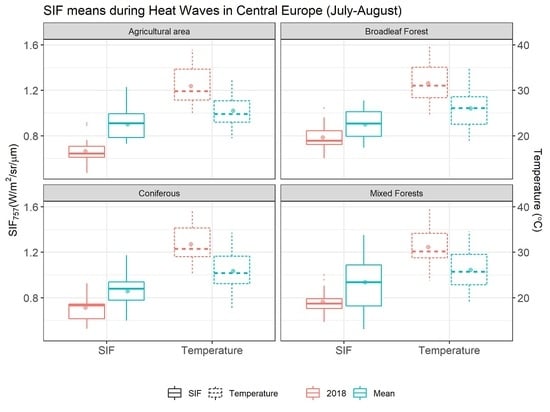
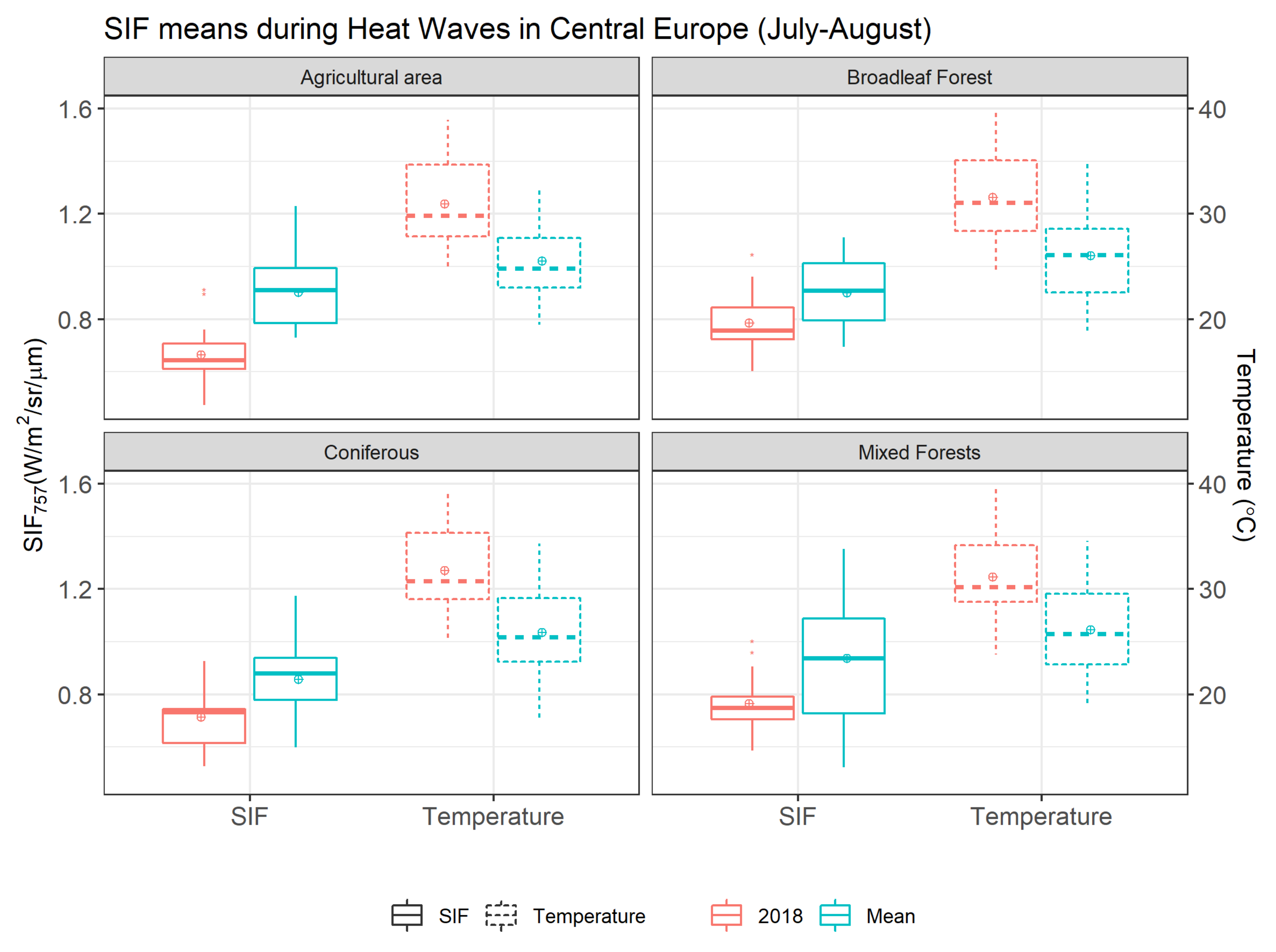
3.3. SIF Variation during the Heatwave

Apart from the extensive drought conditions, Central Europe (i.e., BEL, NLD, DEN, and DEU) was also largely affected by the 2018 heatwave, which was characterized by unusually high temperature anomalies (+5–8 °C) from mid-July to mid-August (Figure 3a). Overall, during this heatwave in Central Europe, the SIF_2018 was 31% lower than SIF_Mean. This difference was most pronounced in agricultural areas which showed 34% lower SIF_2018 followed by mixed forest (25%), coniferous (22%), and broadleaved forest (16%) (Figure 5).

4. Discussion

4.1. Drought Impact on SIF

Our study showed a clear impact of the European hotter drought of 2018 on overall and intra-seasonal SIF variation for different vegetation types as captured by the OCO-2 SIF. Early spring of 2018 was characterized by lower than average temperatures and VPD (i.e., non-stressed stage) followed by above-average temperatures and VPD in the later part of spring (April–May; Figure 3b). Such cooler and wetter conditions in early spring can result in poor crop development and lower productivity [65] and thus lower SIF values ([66]; Figure 3b). Moreover, the initially cooler conditions in spring might have delayed the leaf flushing in deciduous trees, resulting in lower SIF values of broadleaved forests (Figure 3b). This pattern was less evident for the coniferous and mixed forests, probably due to the presence of evergreen trees. In addition, the wet conditions during early spring most likely built up enough soil moisture for the later spring season, thus moderating the sudden warming in later spring season [67,68]. This combination of ample moisture supply with a rise in temperature resulted in an increase in SIF to above-average values across all vegetation types (Figure 3 and Figure 6). The variation in SIF depends on the variation of both APAR (and fPAR) and SIFyield (Equation (1), [69]). Both SIF and fPAR were increasing during the spring season for both drought and non-drought areas (Figure 3 and Figure 4, Figures S4a and S5a). Moreover, for agriculture areas affected by drought, the peaks of fPAR and SIF were on almost the same day of the year (DOY ~ 145; Figure 3a and Figure S4a). However, this clear synchronicity was not found for forests. Nevertheless, we conclude that the satellite-based SIF variation was closely coupled with fPAR variation under non-stress conditions (spring for drought areas and for non-drought areas in spring and summer). Previous studies [13,31,32] have also highlighted the synchronicity of satellite-based SIF with fPAR.
The warming during late spring continued to the summer season, with the later summer season featuring intense heat. We found decreasing SIF in all investigated vegetation types in the summer of 2018, which was most pronounced in the drought areas. The agricultural areas expressed an immediate decrease in SIF from early summer onwards most likely because of severe soil moisture deficits caused by early water depletion in late spring in course of dry weather conditions [70,71]. Ongoing drought conditions during the summer season showed continuous decrease in SIF for agricultural areas and with some delay in forests (Figure 3). Similar findings were reported by an NDVI-based study where agricultural areas, and with some delay, forests in central Europe, faced severe decline in NDVI during the summer season [6]. Unlike agricultural crops, forests feature a buffered microclimate [72,73,74], and given their deeper rooting system in comparison to crops, they have access to deeper soil water and thus can maintain constant photosynthesis rates for extended periods during drought conditions [75].
Our spring–summer seasonal variation of SIF in 2018 is in close agreement with the one of MODIS NDVI ([6]) for agricultural areas. However, for the forest ecosystems, we found a less extreme SIF decline compared to the NDVI-decline in Buras et al. [6]. To further evaluate this difference we analyzed MODIS NDVI over 4 years (2015–2018), and our results indicate that SIF showed higher sensitivity compared to NDVI over the 4-year period (Figure S4b and Figure 6). We observed that for the forest ecosystems in the drought area, fPAR- and NDVI-anomalies were positive during the summer season (DOY < 215) (Figure S4b and Figure 6), i.e., when the SIF-anomaly was reportedly negative. While Buras et al. [6] used a reference period spanning 2000–2018, where several normal and even moist summers were observed, the analyses presented here rely on the 2015–2017 period due to the comparably shorter mission length of OCO-2. However, in 2015 another severe drought hit central and southern Europe, which might have resulted in forest legacy effects [76], i.e., low productivity and die-back in affected areas in 2016 [77]. Consequently, regarding forests, the fPAR and NDVI values from 2018 do only marginally differ to the period mean (2015–2017) since forests could have been suffering at least in 2015 and 2016, i.e., in 2 of the 3 years included in the reference mean. It is, therefore, not surprising that the extremeness of 2018 in the 4 year NDVI analysis of forests (Figure S4 and Figure 6) did not capture the forest decline as clearly as in Buras et al. [6] (with a 19-year reference period) where the majority of reference years represent years with sufficient water supply. In contrast to NDVI over the four years period, SIF was considerably lower in 2018 compared to the already low mean of the previous three years (2015–2017), which may indicate its higher sensitivity to both physiological and structural drought response from plants [32]. This finding highlights the predominance of SIF over NDVI even if short reference periods are available, for example, SIF available from OCO-2, the upcoming OCO-3, and the TROPOMI in comparison to ESA’s SENTINEL-2A [78] (for NDVI).
Vegetation indices (VIs), such as the NDVI, are sensitive to canopy structure and pigment concentration with no direct link to photosynthesis [79]. This might lead to a reduced sensitivity of these VIs to capture drought impact when the vegetation, such as high density forests, still remains green (no changes in chlorophyll content) but reduces its photosynthesis initially during heavily stressed drought conditions [80] in early summer during the European hotter drought. Similar conditions might also not have resulted in significant differences of NDVI during the early summer of 2018 from the mean (Figure S4b). Alternatively, higher sensitivity of SIF (with direct links to photosynthesis) to drought impact on high density European forest was evident from our study (Figure 3 and Figure 6).
The intense heatwave in Central Europe during July and August resulted in a significant decrease in SIF across all the four vegetation types, which was particularly pronounced for agricultural areas. The heatwave occurred at the end of the already dry summer, which was preceded by a dry spring. As a consequence of persisting drought, many crops desiccated, thus not emitting any fluorescence by the end of July when temperatures were extremely high in Central Europe. Water stress due to high-temperature anomalies during a drought event can further increase heat stress due to an extended period of stomatal closure and subsequent reduction in evaporative cooling [81], thus causing positive feedback resulting in even warmer conditions [82].

4.2. SIF Response during Drought Stress

Water stress adversely impacts photosynthesis, either physiologically or structurally [83]. Physiological alterations include change in leaf biochemistry via reductions in enzymatic activity [84] or a reduction in mesophyll/chlorophyll, and stomatal conductance [85], resulting in lower CO2 uptake by the plants and thus reduced photosynthesis (i.e., lower SIF values). The structural changes include foliar changes like leaf wilting or rolling (changes in leaf inclination), thus reducing effective leaf area index (LAI), which in turn causes a reduction in fPAR and energy available for photosynthesis and fluorescence emission [69,86]. Furthermore, plants adopt different mechanisms to minimize water and heat stress, such as chloroplast avoidance movement, during which plants move their chloroplast from the cell surface to side walls of cell [87] so as to minimize APAR [88] and thus SIF. MODIS fPAR decreases due to these protection mechanism, and physiological and structural changes were visible for agricultural areas during the summer drought (Figure S4 and Figure 6). However, for the forest areas we found that MODIS fPAR for drought areas during midsummer (DOY 185–215) was not lower than fPAR in the previous 3 years (Figure 6 and Figure S4). This might imply that a reduction of SIF is likely caused by a reduction in SIFyield. SIF variation due to changes in SIFyield can be because of the canopy’s physiological (ΦF term of Equation (1)) or structural change (ΩC term of Equation (1)), or both. The PAR absorbed by leaves is partitioned into photochemistry, heat dissipation (NPQ), and fluorescence emission (SIF). Although fPAR (or APAR) did not decrease, the proportion of fPAR (or APAR) that is used in photochemistry (to drive electron transport for carbon assimilation) decreases, resulting in a surplus of photosynthetic energy. Now, two other pathways compete to de-excite the absorbed light that is not used in photochemistry (i.e., the surplus photosynthetic energy), the energy emitted as SIF or energy dissipated as heat through NPQ [69]. The competition between these two pathways depends on environmental stress [89], and during water stress conditions (drought), the reduction in SIF is linked to higher NPQ [66,90]. This increase in NPQ may result in a weak coupling between SIF/SIFyield and fPAR under water stress conditions (see Figure S8), which seems to be clearly visible for coniferous and mixed forests during midsummer (DOY 185–215; Figure S4). It is also possible that the MODIS fPAR could be erroneous [32] and not be the best estimate of fPAR, especially in case of high vegetation density (as in Europe). The backup algorithm of MODIS fPAR relies on its relationship with NDVI [49], which becomes nonlinear with a sharp drop of NDVI sensitivity to fPAR for moderate to high vegetation density for fPAR values beyond 0.7 (Figure S6). Nevertheless, further research to differentiate the canopy escape term (ΩC term of Equation (1)) from SIF (as demonstrated by [91,92]) to study changes in fluorescence yield (ΦF) (and SIFyield) during extreme large scale drought event is recommended.
Our results highlight one more reason why OCO-2 SIF can be useful to study drought impact on vegetation as different vegetation types have different responses to drought, which was not efficiently captured for each vegetation types before because of the coarser resolution of preceding satellite-based SIF data/products. We would like to stress that earlier studies used SIF at coarser spatial resolutions (from GOME-2 or GOSAT) and mostly were not able to differentiate SIF responses for different vegetation types from a heterogeneous land-use area during drought conditions. Nevertheless, regarding the drought response of homogeneous vegetation types, our results are in line with previous SIF-based drought impact studies [31,32].

4.3. OCO-2 SIF for Studying Drought Impact

OCO-2 with its increased data acquisition frequency and high spatial resolution was shown to be a promising tool to study large-scale drought impact on vegetation. Although the local pass time of 1:30 PM of OCO-2, allows for a more accurate estimate of SIFyield sensitivity to physiological plant water stress [46], there is a possibility of overestimation of this sensitivity during drought conditions. A combination of derived, improved SIF retrievals from GOME-2 (e.g., SIFTER, [33]), which has a local pass time of 9:30 AM, and OCO-2 should be used to explore and understand the morning–afternoon SIF variation during drought conditions. To better understand the mechanism of stress-induced fluorescence yield variation as captured by the OCO-2 SIF, models that explicitly represent SIF processes (e.g., SCOPE model) should be applied [31,93,94].
The OCO-2 satellite provides a finer spatial resolution SIF data at the cost of temporal resolution (revisit time of 16 days). This might lead to errors due to sampling effects for drought impact studies, especially when comparing with MODIS composite products, as the OCO-2 SIF represents an instantaneous measurement (at 1 PM) performed every 16 days, whereas the MODIS composite represents the best value over a period (mostly 16 or 8 days). This sampling effect might also explain the two peaks in SIF data in broadleaved forest (Figure S7), and this effect is not observed in the NDVI data (Figure S4). However, in our study we deem this effect to be negligible as phenological changes in broadleaf forest during the spring warming of 2018 was well captured despite (Figure 4 and Figure S7) a low and dispersed representation of only 4% of the total study area (Table S3). Moreover, the SIF footprint location keeps changing during every revisit, as the satellite does not operate in a typical “pushbroom” fashion as other sun-synchronous satellites like Sentinel, Landsat, MODIS, etc. This does not allow for a pixel-based temporal analysis of the SIF data. However, with a higher data acquisition rate, this provides a great potential to study large-scale events [42]. Furthermore, a large-scale spatial aggregation of OCO-2 SIF also reduces the uncertainty in OCO-2 SIF measurement owning to higher clear-sky data acquisition rate [42].
Our study also demonstrates the strong added value of SIF-products in comparison to more conventionally used products (NDVI, fPAR), when considering short reference periods (Figure 6 and Figure S4). Moreover, the new sensor of the OCO family (OCO-3) was recently launched on 3 May 2019, which has the same physical and measurement characteristics as compared to OCO-2. With this, a longer time series of high temporal frequency and spatial resolution SIF will be available in the near future. As presented in this study, OCO-2 SIF is sensitive to drought and can serve as a promising and potentially better satellite-based alternative to study impact of extreme events (droughts/floods/heatwaves) on terrestrial ecosystems. To further validate the potential of OCO’s SIF for such studies, a combination of satellite derived vegetation indices, photochemical reflectance index (PRI), SIF (e.g., TROPOMI), and flux data could be considered. A more in-depth site-based study is also recommended to get more insight into ecophysiological stress mechanism in forests during drought. Furthermore, an interpolation of OCO’s dataset through machine learning and statistical tools [34,95] to cover the vacant areas may provide solutions for more rigorous analyses.

5. Conclusions

This study employed the satellite-based SIF measurements acquired from the recent OCO-2 satellite to study the impact of the 2018 European hotter drought on terrestrial ecosystems. Evidently, OCO-2 SIF displayed the spatial and temporal dynamics of the 2018 European drought across different vegetation types (agricultural area, broadleaved forest, coniferous forest, and mixed forest). Our results show that the agricultural areas were severely affected by the 2018 European hotter drought. While the SIF of forests showed a less strong reduction, legacy effects may become visible in the next years and thus, we recommend closely monitoring their behavior. In general, the impact of the heatwave in Central Europe during the July–August period showed an overall 31% decrease in SIF compared to the reference mean. The SIF variation was closely explained by fPAR variation during non-stressed conditions. However, during water-stress conditions (drought), the SIF variation was attributed to variation in SIFyield. Despite a few technical limitations of the OCO-2 SIF measurement such as the 16-day repeat cycle, it provides an excellent potential to study large-scale vegetation fluorescence variation at high spatial resolution and can improve our understanding of changes in ecosystem productivity during extreme events. Furthermore, owing to its direct origin from chlorophyll, OCO-2 SIF can serve as a complementary dataset to MODIS’s vegetation indices (NDVI/EVI). We suggest a more detailed comparison of vegetation indices and OCO-2 SIF to establish the latter’s sensitivity to vegetation’s structural and physiological changes. Further application of OCO-2 SIF may include process-based SCOPE modeling to understand the variation of complex fluorescence yield due to different environmental stress, as well as its combination with the XCO2 data (main product of OCO-2 satellite) to study regional carbon budgets.

Supplementary Materials

The following are available online at https://www.mdpi.com/2072-4292/12/19/3249/s1. Table S1: Relative vegetation class area in percentage for drought and non-drought area. Table S2: Percentage of Nadir OCO-2 measurements mode for the Mean years (2015-2017) and 2018, from total OCO-2 measurements (Nadir + Glint) mode used in the study. Table S3: Comparison of anomalies (2018 – Mean*) in GSIF and OCO-2 SIF measurement (used in this study) for three different areas. Figure S1: Illustration of the spatial distribution and orbit track of OCO-2 SIF soundings of spring and summer season for Europe in 2018. Figure S2: Land cover map of Europe showing agriculture, broadleaf forest, coniferous forest and mixed forest based on Corine Land Cover (CLC) 2018, version 20b2. Figure S3: Representation of climatic water balance (CWB) by the SPEI-3 values during spring (May month) and summer (August month). Figure S4: Variation of (a) fPAR and (b) NDVI for drought area across different vegetation types as observed from MODIS fPAR product (MYD15A2H) version 6 and MODIS NDVI product (MOD/MYD13Q1) version 6. Figure S5: Variation of (a) fPAR and (b) NDVI for non-drought area across different vegetation types as observed from MODIS fPAR product (MYD15A2H) version 6 and MODIS NDVI product (MOD/MYD13Q1) version 6. Figure S6: Relationship between fPAR and NDVI for different vegetation types. Figure S7: Two peaks in the broadleaved forest during summer resulting from a different timing in leaf flushing in the warm summer (Central Europe, blue box) and cool summer (Northern Europe, green box) climate zones of the drought area. Figure S8: Relationship between SIFyield and fPAR across different vegetation types.

Author Contributions

A.S.: Conceptualization, methodology, software, writing—original draft, formal analysis, visualization, funding acquisition. J.C.: Conceptualization, methodology, writing—review and editing, resources, supervision, funding acquisition, project administration. S.B.: Conceptualization, writing—review and editing. A.B.: Conceptualization, methodology, writing—review and editing. A.O.C.: Visualization, resources. C.S.Z.: Methodology, writing—review and editing. A.R.: Conceptualization, methodology, writing—review and editing, supervision, funding acquisition. All authors have read and agreed to the published version of the manuscript.

Funding

This research was funded by Deutscher Akademischer Austauschdienst (DAAD), funding program ID: India IIT Master Sandwich Programme (IIT), 2018 (57434206). The APC was funded by Technical University of Munich-Institute for Advanced Study through the German Excellence Initiative and the European Union Seventh Framework Program under Grant Nr. 291763 and in part by the German Research Foundation (DFG) under Grant Nr. 419317138.

Acknowledgments

The authors would like to immensely thank the OCO-2 team for providing such a valuable dataset. The authors would like to extend its gratitude to the Deutscher Akademischer Austauschdienst (DAAD) and Centre of Rivers Atmosphere and Land Sciences (CORAL), IIT Kharagpur, for funding the research stay at the Technical University of Munich, and to Phillip Papastefanou for his discussion on different drought-induced plant physiological responses. This work was conducted while Ankit Shekhar was with Professorship of environmental sensing and modeling, Technical University of Munich. Now he is at ETH Zürich.

Conflicts of Interest

The authors declare no conflict of interest.

References

  1. IPCC. Summary for Policymakers. In Climate Change 2013: Contribution of Working Group I to the Fifth Assessment Report of the Intergouvernemental Panel on Climate Change; Cambridge University Press: Cambridge, UK; New York, NY, USA, 2018. [Google Scholar]
  2. Dosio, A.; Mentaschi, L.; Fischer, E.M.; Wyser, K. Extreme Heat Waves Under 1.5 °C and 2 °C Global Warming. Environ. Res. Lett. 2018, 13, 054006. [Google Scholar] [CrossRef] [Green Version]
  3. Lhotka, O.; Kysely, J.; Farda, A. Climate Change Scenarios of Heat Waves in Central Europe and Their Uncertainties. Theor. Appl. Clim. 2017, 131, 1043–1054. [Google Scholar] [CrossRef]
  4. Van Loon, A.F.; Gleeson, T.; Clark, J.; Van Dijk, A.I.J.M.; Stahl, K.; Hannaford, J.; Di Baldassarre, G.; Teuling, A.J.; Tallaksen, L.M.; Uijlenhoet, R.; et al. Drought in the Anthropocene. Nat. Geosci. 2016, 9, 89–91. [Google Scholar] [CrossRef] [Green Version]
  5. Allen, C.D.; Breshears, D.D.; McDowell, N.G. On Underestimation of Global Vulnerability to Tree Mortality and Forest Die-off from Hotter Drought in the Anthropocene. Ecosphere 2015, 6, art129. [Google Scholar] [CrossRef]
  6. Buras, A.; Rammig, A.; Zang, C. Quantifying Impacts of the 2018 Drought on European Ecosystems in Comparison to 2003. Biogeosciences 2020, 17, 1655–1672. [Google Scholar] [CrossRef] [Green Version]
  7. Shekhar, A.; Bhattacharjee, S.; Chen, J.; Rammig, A. Spring-Summer Variation Analysis in OCO-2’s Solar Induced Fluorescence During the European Heatwave in 2018. In Geophysical Research Abstracts; Copernicus Publications: Gottingen, Germany, 2019. [Google Scholar]
  8. Heatwave in Northern Europe, Summer 2018. Available online: https://www.worldweatherattribution.org/attribution-of-the-2018-heat-in-northern-europe/ (accessed on 10 August 2020).
  9. Ciais, P.; Reichstein, M.; Viovy, N.; Granier, A.; Ogée, J.; Allard, V.; Aubinet, M.; Buchmann, N.; Bernhofer, C.; Carrara, A.; et al. Europe-Wide Reduction in Primary Productivity Caused by the Heat and Drought in 2003. Nature 2005, 437, 529–533. [Google Scholar] [CrossRef]
  10. Phillips, O.L.; Aragão, L.E.O.C.; Lewis, S.L.; Fisher, J.B.; Lloyd, J.; Lopez-Gonzalez, G.; Malhi, Y.; Monteagudo, A.; Peacock, J.; Quesada, C.A.; et al. Drought Sensitivity of the Amazon Rainforest. Science 2009, 323, 1344–1347. [Google Scholar] [CrossRef] [Green Version]
  11. Beer, C.; Reichstein, M.; Tomelleri, E.; Ciais, P.; Jung, M.; Carvalhais, N.; Rödenbeck, C.; Arain, M.A.; Baldocchi, D.; Bonan, G.B.; et al. Terrestrial Gross Carbon Dioxide Uptake: Global Distribution and Covariation with Climate. Science 2010, 329, 834–838. [Google Scholar] [CrossRef] [Green Version]
  12. Lawrence, D.M.; Oleson, K.W.; Flanner, M.G.; Thornton, P.E.; Swenson, S.; Lawrence, P.J.; Zeng, X.; Yang, Z.-L.; Levis, S.; Sakaguchi, K.; et al. Parameterization Improvements and Functional and Structural Advances in Version 4 of the Community Land Model. J. Adv. Model. Earth Syst. 2011, 3. [Google Scholar] [CrossRef]
  13. Li, X.; Xiao, J.; He, B. Chlorophyll Fluorescence Observed by OCO-2 Is Strongly Related to Gross Primary Productivity Estimated From Flux Towers in Temperate Forests. Remote Sens. Environ. 2018, 204, 659–671. [Google Scholar] [CrossRef]
  14. Smith, W.K.; Biederman, J.A.; Scott, R.L.; Moore, D.J.P.; He, M.; Kimball, J.S.; Yan, D.; Hudson, A.; Barnes, M.L.; MacBean, N.; et al. Chlorophyll Fluorescence Better Captures Seasonal and Interannual Gross Primary Productivity Dynamics Across Dryland Ecosystems of Southwestern North America. Geophys. Res. Lett. 2018, 45, 748–757. [Google Scholar] [CrossRef]
  15. Sun, Y.; Frankenberg, C.; Wood, J.; Schimel, D.S.; Jung, M.; Guanter, L.; Drewry, D.; Verma, M.; Porcar-Castell, A.; Griffis, T.; et al. OCO-2 Advances Photosynthesis Observation From Space via Solar-Induced Chlorophyll Fluorescence. Science 2017, 358, eaam5747. [Google Scholar] [CrossRef] [PubMed] [Green Version]
  16. Xiao, J.; Li, X.; He, B.; Arain, M.A.; Beringer, J.; Desai, A.R.; Emmel, C.; Hollinger, D.Y.; Krasnova, A.; Mammarella, I.; et al. Solar-Induced Chlorophyll Fluorescence Exhibits a Universal Relationship with Gross Primary Productivity Across a Wide Variety of Biomes. Glob. Chang. Boil. 2019, 25, 4. [Google Scholar] [CrossRef] [PubMed] [Green Version]
  17. Yang, X.; Tang, J.; Mustard, J.F.; Lee, J.-E.; Rossini, M.; Joiner, J.; Munger, J.W.; Kornfeld, A.; Richardson, A.D. Solar-Induced Chlorophyll Fluorescence That Correlates With Canopy Photosynthesis on Diurnal and Seasonal Scales in a Temperate Deciduous Forest. Geophys. Res. Lett. 2015, 42, 2977–2987. [Google Scholar] [CrossRef]
  18. Baker, N.R. Chlorophyll Fluorescence: A Probe of Photosynthesis In Vivo. Annu. Rev. Plant. Boil. 2008, 59, 89–113. [Google Scholar] [CrossRef] [Green Version]
  19. Meroni, M.; Rossini, M.; Guanter, L.; Alonso, L.; Rascher, U.; Colombo, R.; Moreno, J. Remote Sensing of Solar-Induced Chlorophyll Fluorescence: Review of Methods and Applications. Remote Sens. Environ. 2009, 113, 2037–2051. [Google Scholar] [CrossRef]
  20. Zarco-Tejada, P.; Morales, A.; Testi, L.; Villalobos, F.J. Spatio-Temporal Patterns of Chlorophyll Fluorescence and Physiological and Structural Indices Acquired From Hyperspectral Imagery as Compared With Carbon Fluxes Measured With Eddy Covariance. Remote Sens. Environ. 2013, 133, 102–115. [Google Scholar] [CrossRef]
  21. Frankenberg, C.; Fisher, J.B.; Worden, J.; Badgley, G.; Saatchi, S.S.; Lee, J.-E.; Toon, G.C.; Butz, A.; Jung, M.; Kuze, A.; et al. New Global Observations of the Terrestrial Carbon Cycle From GOSAT: Patterns of Plant Fluorescence With Gross Primary Productivity. Geophys. Res. Lett. 2011, 38, 1–6. [Google Scholar] [CrossRef] [Green Version]
  22. Guanter, L.; Zhang, Y.; Jung, M.; Joiner, J.; Voigt, M.; Berry, J.A.; Frankenberg, C.; Huete, A.R.; Zarco-Tejada, P.; Lee, J.-E.; et al. Global and Time-Resolved Monitoring of Crop Photosynthesis With Chlorophyll Fluorescence. Proc. Natl. Acad. Sci. USA 2014, 111, E1327–E1333. [Google Scholar] [CrossRef] [Green Version]
  23. Joiner, J.; Vasilkov, A.P.; Yoshida, Y.; Corp, L.A.; Middleton, E.M. First Observations of Global and Seasonal Terrestrial Chlorophyll Fluorescence From Space. Biogeosciences 2011, 8, 637–651. [Google Scholar] [CrossRef] [Green Version]
  24. Parazoo, N.C.; Bowman, K.; Fisher, J.B.; Frankenberg, C.; Jones, D.B.A.; Cescatti, A.; Priego, Ó.P.; Wohlfahrt, G.; Montagnani, L. Terrestrial Gross Primary Production Inferred From Satellite Fluorescence and Vegetation Models. Glob. Chang. Boil. 2014, 20, 3103–3121. [Google Scholar] [CrossRef] [PubMed]
  25. Sanders, A.F.J.; Verstraeten, W.W.; Kooreman, M.L.; Van Leth, T.C.; Beringer, J.; Joiner, J. Spaceborne Sun-Induced Vegetation Fluorescence Time Series from 2007 to 2015 Evaluated with Australian Flux Tower Measurements. Remote Sens. 2016, 8, 895. [Google Scholar] [CrossRef] [Green Version]
  26. Verma, M.; Schimel, D.; Evans, B.; Frankenberg, C.; Beringer, J.; Drewry, D.T.; Magney, T.S.; Marang, I.; Hutley, L.B.; Moore, C.; et al. Effect of Environmental Conditions on the Relationship Between Solar-Induced Fluorescence and Gross Primary Productivity at an Ozflux Grassland Site. J. Geophys. Res. Biogeosciences 2017, 122, 716–733. [Google Scholar] [CrossRef] [Green Version]
  27. Wood, J.; Griffis, T.; Baker, J.; Frankenberg, C.; Verma, M.; Yuen, K. Multiscale Analyses of Solar-Induced Florescence and Gross Primary Production. Geophys. Res. Lett. 2017, 44, 533–541. [Google Scholar] [CrossRef]
  28. Zhang, Y.; Guanter, L.; Berry, J.A.; Joiner, J.; Van Der Tol, C.; Huete, A.R.; Gitelson, A.; Voigt, M.; Köhler, P. Estimation of Vegetation Photosynthetic Capacity From Space-Based Measurements of Chlorophyll Fluorescence for Terrestrial Biosphere Models. Glob. Chang. Boil. 2014, 20, 3727–3742. [Google Scholar] [CrossRef] [PubMed] [Green Version]
  29. Frankenberg, C.; O’Dell, C.; Berry, J.; Guanter, L.; Joiner, J.; Köhler, P.; Pollock, R.; Taylor, T. Prospects for Chlorophyll Fluorescence Remote Sensing from the Orbiting Carbon Observatory-2. Remote Sens. Environ. 2014, 147, 1–12. [Google Scholar] [CrossRef] [Green Version]
  30. Lee, J.-E.; Frankenberg, C.; Van Der Tol, C.; Berry, J.A.; Guanter, L.; Boyce, C.K.; Fisher, J.B.; Morrow, E.; Worden, J.R.; Asefi, S.; et al. Forest Productivity and Water Stress in Amazonia: Observations from Gosat Chlorophyll Fluorescence. Proc. R. Soc. B: Boil. Sci. 2013, 280, 20130171. [Google Scholar] [CrossRef] [Green Version]
  31. Yoshida, Y.; Joiner, J.; Tucker, C.; Berry, J.; Lee, J.-E.; Walker, G.; Reichle, R.; Koster, R.; Lyapustin, A.; Wang, Y. The 2010 Russian Drought Impact on Satellite Measurements of Solar-Induced Chlorophyll Fluorescence: Insights From Modeling and Comparisons with Parameters Derived From Satellite Reflectances. Remote Sens. Environ. 2015, 166, 163–177. [Google Scholar] [CrossRef]
  32. Sun, Y.; Fu, R.; Dickinson, R.; Joiner, J.; Frankenberg, C.; Gu, L.; Xia, Y.; Fernando, D.N. Drought Onset Mechanisms Revealed by Satellite Solar-Induced Chlorophyll Fluorescence: Insights From Two Contrasting Extreme Events. J. Geophys. Res. Biogeosciences 2015, 120, 2427–2440. [Google Scholar] [CrossRef]
  33. Koren, G.; Van Schaik, E.; Araújo, A.C.; Boersma, K.F.; Gärtner, A.; Killaars, L.; Kooreman, M.L.; Kruijt, B.; Luijkx, I.T.; Von Randow, C.; et al. Widespread Reduction in Sun-Induced Fluorescence From the Amazon during the 2015/2016 El Niño. Philos. Trans. R. Soc. B: Boil. Sci. 2018, 373, 20170408. [Google Scholar] [CrossRef]
  34. Zhang, Y.; Joiner, J.; Alemohammad, S.H.; Zhou, S.; Gentine, P. A Global Spatially Contiguous Solar-Induced Fluorescence (CSIF) Dataset Using Neural Networks. Biogeosciences 2018, 15, 5779–5800. [Google Scholar] [CrossRef] [Green Version]
  35. Vicente-Serrano, S.M.; Beguería, S.; López-Moreno, J.I. A Multiscalar Drought Index Sensitive to Global Warming: The Standardized Precipitation Evapotranspiration Index. J. Clim. 2010, 23, 1696–1718. [Google Scholar] [CrossRef] [Green Version]
  36. NOAA National Centers for Environmental Information State of the Climate. Global Climate Report for August 2018; NCEI: Asheville, NC, USA, 2018. [Google Scholar]
  37. NOAA National Centers for Environmental Information State of the Climate. Global Climate Report for July 2018; NCEI: Asheville, NC, USA, 2018. [Google Scholar]
  38. Damm, A.; Elbers, J.; Erler, A.; Gioli, B.; Hamdi, K.; Hutjes, R.; Košvancová, M.; Meroni, M.; Miglietta, F.; Moersch, A.; et al. Remote Sensing of Sun-Induced Fluorescence to Improve Modeling of Diurnal Courses of Gross Primary Production (GPP). Glob. Chang. Boil. 2010, 16, 171–186. [Google Scholar] [CrossRef]
  39. Damm, A.; Guanter, L.; Paul-Limoges, E.; Van Der Tol, C.; Hueni, A.; Buchmann, N.; Eugster, W.; Ammann, C.; Schaepman, M.E. Far-Red Sun-Induced Chlorophyll Fluorescence Shows Ecosystem-Specific Relationships to Gross Primary Production: An Assessment Based on Observational and Modeling Approaches. Remote Sens. Environ. 2015, 166, 91–105. [Google Scholar] [CrossRef]
  40. Frankenberg, C.; Berry, J. Solar Induced Chlorophyll Fluorescence: Origins, Relation to Photosynthesis and Retrieval; Elsevier: Amsterdam, The Netherlands, 2018; pp. 143–162. [Google Scholar]
  41. Frankenberg, C.; Butz, A.; Toon, G.C. Disentangling Chlorophyll Fluorescence From Atmospheric Scattering Effects in O2 A Band Spectra of Reflected Sun-Light. Geophys. Res. Lett. 2011, 38. [Google Scholar] [CrossRef]
  42. Sun, Y.; Frankenberg, C.; Jung, M.; Joiner, J.; Guanter, L.; Köhler, P.; Magney, T.S. Overview of Solar-Induced Chlorophyll Fluorescence (SIF) from the Orbiting Carbon Observatory-2: Retrieval, Cross-Mission Comparison, and Global Monitoring for GPP. Remote Sens. Environ. 2018, 209, 808–823. [Google Scholar] [CrossRef]
  43. Shekhar, A.; Chen, J.; Paetzold, J.C.; Dietrich, F.; Zhao, X.; Bhattacharjee, S.; Ruisinger, V.; Wofsy, S.C. Anthropogenic CO2 Emissions Assessment of Nile Delta Using XCO2 and Sif Data From OCO-2 Satellite. Environ. Res. Lett. 2020, 15, 095010. [Google Scholar] [CrossRef]
  44. Frankenberg, C. Solar Induced Chlorophyll Fluorescence: OCO-2 Lite Files (B7000) User Guide; California Institute of Technology: Pasadena, CA, USA, 2015. [Google Scholar]
  45. Zhang, Z.; Zhang, Y.; Joiner, J.; Migliavacca, M. Angle Matters: Bidirectional Effects Impact the Slope of Relationship Between Gross Primary Productivity and Sun-Induced Chlorophyll Fluorescence From Orbiting Carbon Observatory-2 Across Biomes. Glob. Chang. Boil. 2018, 24, 5017–5020. [Google Scholar] [CrossRef] [Green Version]
  46. Goulas, Y.; Daumard, F.; Ounis, A.; Rhoul, C.; Lopez, M.L.; Moya, I. Monitoring the Diurnal Time Course of Vegetation Dynamics with Geostationary Observations: The Gflex Project. In Proceedings of the 6th Workshop on Hyperspectral Image and Signal Processing: Evolution in Remote Sensing (WHISPERS), Laussane, Switzerland, 24–27 June 2014; pp. 1–4. [Google Scholar] [CrossRef]
  47. Yan, K.; Park, T.; Yan, G.; Chen, C.; Yang, B.; Liu, Z.; Nemani, R.R.; Knyazikhin, Y.; Myneni, R.B. Evaluation of MODIS LAI/FPAR Product Collection 6. Part 1: Consistency and Improvements. Remote Sens. 2016, 8, 359. [Google Scholar] [CrossRef] [Green Version]
  48. Yan, K.; Park, T.; Yan, G.; Liu, Z.; Yang, B.; Chen, C.; Nemani, R.R.; Knyazikhin, Y.; Myneni, R.B. Evaluation of MODIS LAI/FPAR Product Collection 6. Part 2: Validation and Intercomparison. Remote Sens. 2016, 8, 460. [Google Scholar] [CrossRef] [Green Version]
  49. Knyazikhin, Y.; Myneni, R.B.; Privette, J.L.; Running, S.W.; Nemani, R.; Zhang, Y.; Tian, Y.; Wang, Y.; Morissette, J.T.; Glassy, J.; et al. MODIS Leaf Area Index (LAI) and Fraction of Photosynthetically Active Radiation Absorbed by Vegetation (FPAR) Product (MOD15) Algorithm Theoretical Basis Document; Boston University: Boston, MA, USA, 1999. [Google Scholar]
  50. Solano, R.; Didan, K.; Jacobson, A.; Huete, A. MODIS Vegetation Index User’s Guide, MOD13 Series; University of Arizona: Tucson, AZ, USA, 2010. [Google Scholar]
  51. Büttner, G.; Kosztra, B. CLC2018 Technical Guidelines; EEA: Wien, Austria, 2017; pp. 1–60. [Google Scholar]
  52. Wable, P.S.; Jha, M.K.; Shekhar, A. Comparison of Drought Indices in a Semi-Arid River Basin of India. Water Resour. Manag. 2018, 33, 75–102. [Google Scholar] [CrossRef]
  53. Nam, W.-H.; Hayes, M.J.; Svoboda, M.D.; Tadesse, T.; Wilhite, D.A. Drought Hazard Assessment in the Context of Climate Change For South Korea. Agric. Water Manag. 2015, 160, 106–117. [Google Scholar] [CrossRef]
  54. Zang, C.; Buras, A.; Esquivel-Muelbert, A.; Jump, A.S.; Rigling, A.; Rammig, A. Standardized Drought Indices in Ecological Research: Why One Size Does Not Fit All. Glob. Chang. Boil. 2019, 26, 322–324. [Google Scholar] [CrossRef] [PubMed] [Green Version]
  55. Ionita, M.; Tallaksen, L.M.; Kingston, D.G.; Stagge, J.H.; Laaha, G.; Van Lanen, H.; Scholz, P.; Chelcea, S.M.; Haslinger, K. The European 2015 Drought From a Climatological Perspective. Hydrol. Earth Syst. Sci. 2017, 21, 1397–1419. [Google Scholar] [CrossRef] [Green Version]
  56. Dong, B.; Sutton, R.T.; Shaffrey, L.; Wilcox, L.J. The 2015 European Heat Wave. Bull. Am. Meteorol. Soc. 2016, 97, S57–S62. [Google Scholar] [CrossRef]
  57. McCornack, R.L. Extended Tables of the Wilcoxon Matched Pair Signed Rank Statistic. J. Am. Stat. Assoc. 1965, 60, 864–871. [Google Scholar] [CrossRef]
  58. KMI. Klimatologisch Maandoverzicht Juli 2018 (PDF); KMI: Brussels, Belgium. (In Dutch)
  59. KNMI—Hittegolf. 2019. Available online: www.knmi.nl (accessed on 10 August 2020).
  60. Danmarks Meteorologiske Institut. Juni bliver den varmeste og solrigeste i 26 år.; DMI: Copenhague, Denmark, 2018. (In Danish) [Google Scholar]
  61. DWD. Deutscher Wetterdienst; DWD: Offenbach, Germany, 2018. [Google Scholar]
  62. R Development Core Team. A Language and Environment for Statistical Computing. R. Found. Stat. Comput. 2011, 1, 409. [Google Scholar]
  63. Wickham, H. ggplot2: Elegant Graphics for Data Analysis; Springer: New York, NY, USA, 2016. [Google Scholar]
  64. Wickham, H.; Francois, R. dplyr: A Grammar of Data Manipulation, R Packag. version 0.4.2; R Studio: Boston, MA, USA, 2015. [Google Scholar]
  65. Shekhar, A.; Shapiro, C.A. What Do Meteorological Indices Tell Us About a Long-Term Tillage Study? Soil Tillage Res. 2019, 193, 161–170. [Google Scholar] [CrossRef]
  66. Paul-Limoges, E.; Damm, A.; Hueni, A.; Liebisch, F.; Eugster, W.; Schaepman, M.E.; Buchmann, N. Effect of Environmental Conditions on Sun-Induced Fluorescence in a Mixed Forest and a Cropland. Remote Sens. Environ. 2018, 219, 310–323. [Google Scholar] [CrossRef]
  67. Miralles, D.G.; Teuling, A.J.; Van Heerwaarden, C.C.; De Arellano, J.V.-G. Mega-Heatwave Temperatures Due to Combined Soil Desiccation and Atmospheric Heat Accumulation. Nat. Geosci. 2014, 7, 345–349. [Google Scholar] [CrossRef]
  68. Sippel, S.; Forkel, M.; Rammig, A.; Thonicke, K.; Flach, M.; Heimann, M.; Otto, F.E.L.; Reichstein, M.; Mahecha, M.D. Contrasting and Interacting Changes in Simulated Spring and Summer Carbon Cycle Extremes in European Ecosystems. Environ. Res. Lett. 2017, 12, 075006. [Google Scholar] [CrossRef]
  69. Porcar-Castell, A.; Tyystjärvi, E.; Atherton, J.; Van Der Tol, C.; Flexas, J.; Pfündel, E.E.; Moreno, J.; Frankenberg, C.; Berry, J.A. Linking Chlorophyll a Fluorescence to Photosynthesis for Remote Sensing Applications: Mechanisms and Challenges. J. Exp. Bot. 2014, 65, 4065–4095. [Google Scholar] [CrossRef] [PubMed]
  70. Crausbay, S.D.; Ramirez, A.R.; Carter, S.L.; Cross, M.S.; Hall, K.R.; Bathke, D.; Betancourt, J.L.; Colt, S.; Cravens, A.E.; Dalton, M.S.; et al. Defining Ecological Drought for the Twenty-First Century. Bull. Am. Meteorol. Soc. 2017, 98, 2543–2550. [Google Scholar] [CrossRef]
  71. Sippel, S.; Zscheischler, J.; Reichstein, M. Ecosystem Impacts of Climate Extremes Crucially Depend on the Timing. Proc. Natl. Acad. Sci. USA 2016, 113, 5768–5770. [Google Scholar] [CrossRef] [Green Version]
  72. Chen, J.; Franklin, J.F.; Spies, T.A. Contrasting Microclimates Among Clearcut, Edge, and Interior of Old-Growth Douglas-Fir Forest. Agric. For. Meteorol. 1993, 63, 219–237. [Google Scholar] [CrossRef]
  73. Chen, J.; Saunders, S.C.; Crow, T.R.; Naiman, R.J.; Brosofske, K.D.; Mroz, G.D.; Brookshire, B.L.; Franklin, J.F. Microclimate in Forest Ecosystem and Landscape Ecology. Bioscience 1999, 49, 288–297. [Google Scholar] [CrossRef] [Green Version]
  74. Young, A.; Mitchell, N. Microclimate and Vegetation Edge Effects in a Fragmented Podocarp-Broadleaf Forest in New Zealand. Boil. Conserv. 1994, 67, 63–72. [Google Scholar] [CrossRef]
  75. Krishnan, P.; Black, T.A.; Grant, N.J.; Barr, A.G.; Hogg, E.; Jassal, R.S.; Morgenstern, K. Impact of Changing Soil Moisture Distribution on Net Ecosystem Productivity of a Boreal Aspen Forest During and Following Drought. Agric. For. Meteorol. 2006, 139, 208–223. [Google Scholar] [CrossRef]
  76. Anderegg, W.R.L.; Schwalm, C.; Biondi, F.; Camarero, J.J.; Koch, G.; Litvak, M.; Ogle, K.; Shaw, J.D.; Shevliakova, E.; Williams, A.P.; et al. Pervasive Drought Legacies in Forest Ecosystems and Their Implications for Carbon Cycle Models. Science 2015, 349, 528–532. [Google Scholar] [CrossRef] [Green Version]
  77. Buras, A.; Schunk, C.; Zeiträg, C.; Herrmann, C.; Kaiser, L.; Lemme, H.; Straub, C.; Taeger, S.; Gößwein, S.; Klemmt, H.-J.; et al. Are Scots Pine Forest Edges Particularly Prone to Drought-Induced Mortality? Environ. Res. Lett. 2018, 13, 025001. [Google Scholar] [CrossRef]
  78. Forstmaier, A.; Shekhar, A.; Chen, J. Mapping of Eucalyptus in Natura 2000 areas using Sentinel 2 imagery and artificial neural networks. Remote Sens. 2020, 12, 2176. [Google Scholar] [CrossRef]
  79. Dobrowski, S.Z.; Pushnik, J.; Zarco-Tejada, P.; Ustin, S. Simple Reflectance Indices Track Heat and Water Stress-Induced Changes in Steady-State Chlorophyll Fluorescence at the Canopy Scale. Remote Sens. Environ. 2005, 97, 403–414. [Google Scholar] [CrossRef]
  80. Wang, S.; Huang, C.; Zhang, L.; Lin, Y.; Cen, Y.; Wu, T. Monitoring and Assessing the 2012 Drought in the Great Plains: Analyzing Satellite-Retrieved Solar-Induced Chlorophyll Fluorescence, Drought Indices, and Gross Primary Production. Remote Sens. 2016, 8, 61. [Google Scholar] [CrossRef] [Green Version]
  81. De Boeck, H.J.; Verbeeck, H. Drought-Associated Changes in Climate and Their Relevance for Ecosystem Experiments and Models. Biogeosciences 2011, 8, 1121–1130. [Google Scholar] [CrossRef] [Green Version]
  82. Fischer, E.M.; Seneviratne, S.I.; Vidale, P.L.; Luthi, D.; Schär, C. Soil Moisture–Atmosphere Interactions during the 2003 European Summer Heat Wave. J. Clim. 2007, 20, 5081–5099. [Google Scholar] [CrossRef]
  83. Chaves, M.M. Effects of Water Deficits on Carbon Assimilation. J. Exp. Bot. 1991, 42, 1–16. [Google Scholar] [CrossRef]
  84. Keenan, T.F.; Sabaté, S.; Gracia, C. The Importance of Mesophyll Conductance in Regulating Forest Ecosystem Productivity During Drought Periods. Glob. Chang. Boil. 2010, 16, 1019–1034. [Google Scholar] [CrossRef]
  85. Bréda, N.; Huc, R.; Granier, A.; Dreyer, E. Temperate Forest Trees and Stands Under Severe Drought: A Review of Ecophysiological Responses, Adaptation Processes and Long-Term Consequences. Ann. For. Sci. 2006, 63, 625–644. [Google Scholar] [CrossRef] [Green Version]
  86. Castro, A.O.; Chen, J.; Zang, C.; Shekhar, A.; Jiménez-Muñoz, J.C.; Bhattacharjee, S.; Kindu, M.; Morales, V.H.; Rammig, A. OCO-2 Solar-Induced Chlorophyll Fluorescence Variability across Ecoregions of the Amazon Basin and the Extreme Drought Effects of El Niño (2015–2016). Remote Sens. 2020, 12, 1202. [Google Scholar] [CrossRef] [Green Version]
  87. Kasahara, M.; Kagawa, T.; Oikawa, K.; Suetsugu, N.; Miyao, M.; Wada, M. Chloroplast Avoidance Movement Reduces Photodamage in Plants. Nature 2002, 420, 829–832. [Google Scholar] [CrossRef]
  88. Field, C.B. Ecological Scaling of Carbon Gain to Stress and Resource Availability. In Response of Plants to Multiple Stresses; Elsevier: Amsterdam, The Netherlands, 1991; pp. 35–65. [Google Scholar]
  89. Flexas, J.; Medrano, H. Drought-inhibition of Photosynthesis in C3 Plants: Stomatal and Non-stomatal Limitations Revisited. Ann. Bot. 2002, 89, 183–189. [Google Scholar] [CrossRef] [PubMed] [Green Version]
  90. Peguero-Pina, J.J.; Morales, F.; Flexas, J.; Gil-Pelegrín, E.; Moya, I. Photochemistry, Remotely Sensed Physiological Reflectance Index and de-Epoxidation State of the Xanthophyll Cycle in Quercus Coccifera Under Intense Drought. Oecologia 2008, 156, 1–11. [Google Scholar] [CrossRef] [PubMed]
  91. Yang, P.; Van Der Tol, C. Linking Canopy Scattering of Far-Red Sun-Induced Chlorophyll Fluorescence with Reflectance. Remote Sens. Environ. 2018, 209, 456–467. [Google Scholar] [CrossRef]
  92. Zeng, Y.; Badgley, G.; DeChant, B.; Ryu, Y.; Chen, M.; Berry, J. A Practical Approach for Estimating the Escape Ratio of Near-Infrared Solar-Induced Chlorophyll Fluorescence. Remote Sens. Environ. 2019, 232, 111209. [Google Scholar] [CrossRef] [Green Version]
  93. Lee, J.-E.; Berry, J.; Van Der Tol, C.; Yang, X.; Guanter, L.; Damm, A.; Baker, I.; Frankenberg, C. Simulations of Chlorophyll Fluorescence Incorporated Into the Community Land Model Version 4. Glob. Chang. Boil. 2015, 21, 3469–3477. [Google Scholar] [CrossRef] [Green Version]
  94. Van Der Tol, C.; Berry, J.A.; Campbell, P.K.E.; Rascher, U. Models of Fluorescence and Photosynthesis for Interpreting Measurements of Solar-Induced Chlorophyll Fluorescence. J. Geophys. Res. Biogeosciences 2014, 119, 2312–2327. [Google Scholar] [CrossRef] [Green Version]
  95. Bhattacharjee, S.; Chen, J. Prediction of Satellite-Based Column CO2 Concentration by Combining Emission Inventory and LULC Information. IEEE Trans. Geosci. Remote Sens. 2020, 1–16. [Google Scholar] [CrossRef]
Figure 1. Drought severity map of Europe in (a) spring (SPEI-3 of May) and (b) summer (SPEI-3 of August) of 2018. The map is based on the Standardized Precipitation Evapotranspiration Index (SPEI) Global Drought Monitor (http://spei.csic.es/index.html). (c) Drought area and non-drought area used in the study. Drought area has 2018 spring and summer SPEI values less than −1. Non-drought area has 2018 spring and summer SPEI values greater than −1.
Remotesensing 12 03249 g001
Figure 2. Overall solar-induced (chlorophyll) fluorescence (SIF) variation in (a) spring and (b) summer season for drought areas in 2018 (SIF_2018, in orange) compared to mean SIF values from 2015–2017 (SIF_Mean, in grey). Bars indicate the histogram of the SIF, whereas curves represent the density plot of the histogram.
Remotesensing 12 03249 g002
Figure 3. (a) Intra-seasonal SIF variability based on a 5-day running mean for drought areas across different vegetation types. (b) Corresponding SIF anomalies (SIF-Diff), and vapor pressure deficit (VPD) (gray line), and temperature (black line) anomalies. Positive values indicate a surplus of SIF, temperature (Temp), and VPD; negative values indicate lower values in comparison to the mean in 2015–2017. Shaded area (light blue for “Mean”; red for “2018”) in part (a) is ± standard error of mean obtained after spatially aggregating the samples. The vertical dashed lines divide the DOY into spring (DOY 60–150) and summer (DOY 151–245) season. Temp-Diff = Temp_2018–Temp_Mean; VPD-Diff = VPD_2018–VPD_Mean.
Remotesensing 12 03249 g003
Figure 4. (a) Intra-seasonal SIF variability based on 5-day running mean for non-drought areas across different vegetation types. (b) Corresponding SIF anomalies (SIF-Diff), and VPD (gray line), and temperature (black line) anomalies. Positive values indicate a surplus of SIF, Temp, and VPD; negative values indicate lower values in comparison to the mean in 2015–2017. Shaded area (light blue for SIF_Mean; red for SIF_2018) in part (a) is ± standard error of mean obtained after spatially aggregating the samples. The vertical dashed lines divide the DOY into spring (DOY 60–150) and summer (DOY 151–240) season. Temp-Diff = Temp_2018–Temp_Mean; VPD-Diff = VPD_2018–VPD_Mean.
Remotesensing 12 03249 g004
Figure 5. Boxplots illustrating SIF variation across the four vegetation type during the heatwave (15 July to 15 August) in central Europe (i.e., Germany, Denmark, Belgium, and Netherlands) along with temperature differences. Dots inside the boxplots represent the corresponding mean values.
Remotesensing 12 03249 g005
Figure 6. Anomalies (in % difference from “Mean”) of SIF, the Normalized Difference Vegetation Index (NDVI), and fPAR for drought area across different vegetation types as observed from the Orbiting Carbon Observatory-2 (OCO-2) SIF, MODIS NDVI product (MOD/MYD13Q1) version 6, and MODIS fPAR product (MYD15A2H) version 6 in 2018. Positive values indicate a surplus of SIF, NDVI, and fPAR, negative values indicate lower values in comparison to the mean in 2015–2017. The left and right side of blue vertical dashed line represents spring and summer season, respectively.
Remotesensing 12 03249 g006
Table 1. European-wide mean SIF_757nm (W/m2/sr/µm) values in spring, summer, and the combined spring–summer season and their corresponding anomaly (SIF-Diff) for whole of Europe, drought area and non-drought area.
Area(a) Combined Spring–Summer(b) Spring(c) Summer
SIF_2018SIF_MeanSIF-DiffSIF_2018SIF_MeanSIF-DiffSIF_2018SIF_MeanSIF-Diff
Europe0.6420.670−0.0280.5230.534−0.0110.7660.820−0.054 *
Drought area0.5580.596−0.0380.4070.3880.0190.7110.814−0.103 *
Non-drought area0.6840.6600.0240.6010.5600.0410.7660.767−0.001
* p-value < 0.001.

