Evaporative Fluxes and Surface Soil Moisture Retrievals in a Mediterranean Setting from Sentinel-3 and the “Simplified Triangle”

Abstract

Earth Observation (EO) makes it possible to obtain information on key parameters characterizing interactions among Earth’s system components, such as evaporative fraction (EF) and surface soil moisture (SSM). Notably, techniques utilizing EO data of land surface temperature (Ts) and vegetation index (VI) have shown promise in this regard. The present study investigates, for the first time, the accuracy of one such technique, known as the “simplified triangle”, using Sentinel-3 EO data, acquired for 44 days in 2018 at three savannah FLUXNET sites in Spain. The technique was found to be able to predict both EF and SSM with reasonable accuracy when compared to collocated ground measurements. Comparisons performed for all days together showed relatively low Root Mean square Difference (RMSD) for both EF (0.191) and SSM (0.012 cm³ cm⁻³) and good correlation coefficients (R) of 0.721 and 0.577, respectively. Both EF and SSM were also largely in agreement with land cover and seasonal variability. The present study comprises the first detailed assessment of the “simplified triangle”, in this case, using Sentinel-3 data and in a Mediterranean setting. Findings, albeit preliminary, are of significant value regarding the use of the investigated technique as a tool of environmental management, and towards ongoing, worldwide efforts aiming at developing operationally relevant products based on the Ts/VI feature space and EO data based on new satellites such as Sentinel-3.

1. Introduction

Earth’s natural processes and the relationships between soil-vegetation and the atmosphere components of the Earth system are topics of great importance for numerous disciplines covering a range of practical applications and research [1,2,3,4]. The need for accurate information on parameters characterizing the environment of the Earth system is even more acute today, in light of increased pressure due to climate change and global challenges linked to global food and water security [5]. Recent climate projections, for example, suggest that the Mediterranean will be subject to severe climate change, including increased temperatures and reduced precipitation [6]. In this context, the accurate monitoring of parameters such as evaporative fraction (i.e., the ratio of instantaneous latent heat flux (LE) to net radiation (Rn)) and surface soil moisture (SSM) is of high priority. Both are essential environmental parameters which play instrumental roles in numerous physical processes, and thereby affect the climate directly or indirectly [7,8,9]. Thus, being able to accurately estimate their changes in both the time and spatial domains is undoubtedly of prime interest for many applications in numerous disciplines [10,11].

Earth Observation (EO) has experienced rapid growth over recent decades, providing a pathway towards acquiring both EF and SSM at variable geographical scales with temporally consistent coverage. A wealth of techniques have been proposed exploiting EO data acquired from across the electromagnetic spectrum to retrieve these parameters (e.g., see reviews by [8,12]. 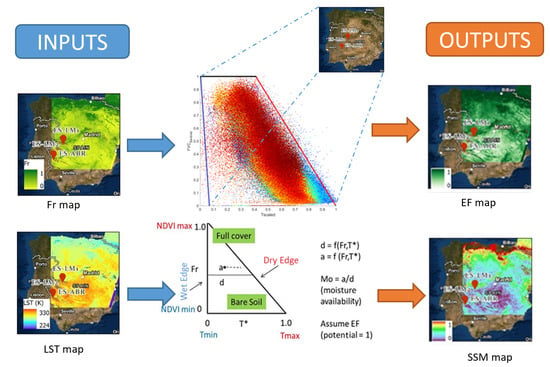Thermal Infrared (TIR) remote sensing, despite its requirement for clear sky conditions, has been the preferred option for both EF and SSM retrievals to date because of its fine resolution in the spatial and temporal domains [13]. A specific group of TIR-based approaches that rely on the physical relationships implied by EO-derived scatterplots in which the surface temperature (Ts) is plotted versus the vegetation index (VI) have shown potential in this respect. Assuming conditions of full variability in vegetation cover in EO-based imagery, a scatterplot is generated with a triangular (or trapezoidal) shape. The emergence of this shape results from the reduced sensitivity that Ts has on water content over areas covered by vegetation in comparison to bare soil areas. A detailed description of the Ts/VI feature space and of the biophysical properties included within it can be found in [14].

Several researchers have already demonstrated how EF and SSM can be derived from the Ts/VI feature space utilizing a range of EO data (e.g., [15,16,17,18,19,20,21,22,23]. The promising potential of Ts/VI techniques is evidenced in the fact that variants are being, or have been, considered by different Space Agencies in the development of operational EO-based products [24,25,26]. A group of these techniques has already demonstrated its ability to provide operational service SSM maps over Spain at 1 km pixel size based on data from the SMOS satellite, integrating the SMOS brightness temperature values within a multiple regression model, together with Ts and VI obtained from the MODIS data [27].

Recently [28] proposed a new technique for estimating both SSM and EF from the Ts/VI domain, named “simplified triangle”. This approach has a major advantage in comparison to other Ts/VI techniques, in that it is based on only a few calculations and does not require for its implementation a mathematical model to simulate physical processes or ancillary data; therefore, it can be easily implemented almost anywhere in the world. As the technique is easy to use and only depends on EO data, it is a prime candidate for operational use. Nevertheless, more research is required to evaluate its performance in different ecosystems and environmental conditions globally, particularly regarding the use of EO data from new satellites such as those from Sentinel-3.

The authors of [29] demonstrated the use of the “simplified” triangle approach coupled with crop prediction and climatological water balance models to predict soybean yield using MODIS data. Yet, to our knowledge, this technique using ESA’s Sentinels-3 has not yet been implemented. Sentinel-3 provides EO data at a range of resolutions in the spatial, temporal and spectral domains. Thus, such satellite observations may serve in many potential applications [30,31].

On this basis, the present research study aims at exploring the ability of the “simplified triangle”, used synergistically with Sentinel-3 data, to predict the spatio-temporal variability of both EF and SSM. To our knowledge, in that respect, this is the first study of its kind. The technique was assessed in two regions in Spain for which validated collocated ground observations from the FLUXNET global in situ monitoring network were available. The next section provides a description of the study area; Section 3 outlines the methods, Section 4 the key results and Section 5 discusses the obtained results.

2. Materials

2.1. Study Sites and In Situ Data

Ground measurements from three Spanish sites that belong to the CarboEurope in situ measurements network were used in this study. CarboEurope belongs to FLUXNET, which is a major ground observational network that acquires land surface parameter data [32,33]. All data collected from the FLUXNET individual sites were first measured using standardized instrumentation across the network sites. Then, quality-controls and uniformly applied error correction processing were applied to them before distribution. In situ data is made available at different processing levels and at no cost from the European Fluxes Database Cluster (http://gaia.agraria.unitus.it/).

Herein, the “simplified triangle” technique is evaluated at three CarboEurope sites in Spain, representative of typical savannah ecosystem types for selected cloud-free days in 2018.

Table 1. Main characteristics of our study sites.

Site Name	Site Abbreviation	Geographic Coordinates (Lat/Long)	Country	Ecosystem Type/Land Cover	Elevation (m)
Albuera	Es-Abr	38.702–6.786	SPAIN	SAV	279
Majadas del Tietar North	Es-LM1	39.942–5.779	SPAIN	SAV	266
Majadas del Tietar South	ES-LM2	39.935–5.776	SPAIN	SAV	270

summarizes the main characteristics of the study sites and the location of each site is illustrated in Figure 1. In total, 44 days from 2018 were chosen to verify the technique. The target criteria for selecting the specific days included cloud-free skies, the availability of good quality in situ data concurrently to the satellite observations and a satisfactory energy balance closure (EBC), which was used as an indication of good quality flux measurements (evaluated as per previous studies such as [34,35]). In our study, days of Sentinel-3 overpass with poor EBC (EBR < 0.750, slope < 0.85, R² < 0.930) were excluded from further analysis, similarly to other studies [36,37].

All ground measurements used in this study were obtained from the ICOS (Integrated Carbon Observation System) database (http://www.europe-fluxdata.eu/icos/home). Detailed information on the data use policy can be found on the CarboEurope website and data acquisition interface. For consistency purposes, all ground data acquired in this study were also obtained at Level 2 processing, meaning that they included the originally acquired measurements from which only incorrect data (e.g., due to instrumentation error) had been eliminated. No further preprocessing was implemented apart from the computation of EF (as defined previously, i.e., LE/Rn).

2.2. Sentinels Data: Acquisition and Preprocessing

Sentinel-3 was launched by the European Space Agency (ESA) as part of the Copernicus Program. At present, it consists of two satellites (Sentinel-3A and 3B) working in constellation, with two additional satellites planned for launch in the near future. One of the instruments onboard the Sentinel-3 platform is a SLSTR (Sea and Land Surface Temperature Radiometer). The launch of the satellites in constellation allows SLSTR to achieve a temporal resolution at the equator of less than a day. Spectrally, the instrument acquires data in a total of nine spectral bands, plus two more which were developed for applications relevant primarily to the monitoring of fires. The first six bands, located from visible to short-wave infrared (SWIR), acquire spectral data at 500 m. Subsequent bands, i.e., bands 7 to 9, have a 1-km spatial resolution. More details on the SLSTR instrument are available elsewhere, for example [38].

Herein, the Sentinel-3 Level 2 operational product, named “SL_2_LST”, is used to implement the “simplified triangle” technique. Based on the delivery time, two data product types are available for the SLSTR Sentinel 3 product. These products are “Near Real Time” (NRT), provided in less than 3 hours after image acquisition, and “Non-Critical Time” (NTC), provided within one month after image acquisition. The main difference between them is the VIS/SWIR calibration applied to the NRT products, which makes them suitable for our current study. The spatial resolution the of LST and VI band is 1 km and the temporal resolution is, at the latitudes of our study area, at least two times per day (once in the morning and once in the afternoon; precise time varies according to orbit and is not geosynchronous). This product provides Land Surface Temperature (LST, or Ts, as defined before) and a series of other parameters to users. The product is organized into packages composed of one manifest file and several measurements and annotation data files (between 2 and 21 files, depending on the package). The SL_2_LST product, in particular, contains ten annotation files, providing the same parameters as SL_2_WCT and some additional vegetation parameters. One of these parameters is the Fractional Vegetation Cover (Fr), which is used to satisfy the objectives of the present study. In SL_2_LST, the vegetation is specified as a fractional vegetation index ranging between ‘1’ (corresponding to 100% vegetation) and ‘0’ (corresponding to 0% vegetation). The LST algorithm used for Sentinel 3 is based on two split-window thermal channels (1100 nm and 1200 nm). The global estimation of the LST takes into account the effects of the land emissivity, together with those of atmospheric water vapor and satellite viewing angle. The LST estimation uses a linear regression with coefficients tailored for day and night, land cover types, various atmospheric conditions, and bare and vegetated surfaces. More details on the Fr and LST Sentinel-3 products can be found elsewhere including open-access documents (e.g., in [39]).

The SL_2_LST images used herein were first obtained from CREODIAS (https://creodias.eu/) at no cost, covering the entire Sentinel-3 image archive initially for the year 2018. Next, specific Sentinel-3 images were selected for inclusion in this study. These included only cloud-free images or images with less than 20% cloud presence in their field of view. Each image from the archive was intersected to each image footprint covering the entire study area. For each SL_2_LST image product that was retained for further analysis, first, spatial and spectral subsets were selected. These covered the studied regions), where the layers retained included only the Ts (or LST), Fr and the Normalised Difference Vegetation Index (NDVI). Then, each band was masked for clouds and inland water. Subsequently, all the study sites were cross-intersected with the images, using an algorithm based on the closest date and time acquisition for in situ and satellite images. The final set of SLs_2_LST images, for a total of 70 days, provided the input data for the implementation of the “simplified triangle”. An example of these final image products for a selected day is given in Figure 2.

3. Methods

3.1. “Simplified Triangle”

The “simplified triangle” is a new Ts/VI technique proposed by [28]. The technique makes it possible to derive spatial estimates of the surface wetness (Mo, which refers to the first few millimeters of a surface covered by bare soil) and of the evaporative fraction (EF, being the ratio of evapotranspiration to net radiation (Rn)). The principle on which the method is based is illustrated in Figure 3. Briefly, the key inputs to the method include the Fr and Ts parameters. The authors of [28] proposed deriving Fr from the scaling of the NDVI. This approach requires specifying NDVI for bare soil (NDVIo), and for full vegetation cover (NDVIs) values (see Figure 3), and is based on the following equation [15,40]:

$$\mathrm{Fr}= {\left\{\frac{\mathrm{NDVI}-{\mathrm{NDVI}}_0}{\mathrm{NDVIs}-{\mathrm{NDVI}}_0}\right\}}^2$$

(1)

However, other methods of Fr estimation can also be used. In the present work, since the Fr layer is included in the Sentinel product, this information was used as the input and no computation was required.

NDVIs and T[min] define the lower left (wet or cold) peak, i.e., the so-called “wet edge” (or “cold edge”), which characterizes dense vegetation (refer to Figure 3). Similarly, NDVIo and T[max] describe the lower right border of the triangle. An additional essential characteristic, the “dry edge” or “warm edge” (also shown in Figure 3), represents the soil dryness limit (i.e., conditions where Mo = 0).

The next step in applying the technique is the scaling of Ts to a variable named T*, resulting in values varying between zero and one. Scaling requires identifying Ts for dry/bare soil, i.e., the maximum Ts [max] value for pixels over dry/bare soil, and the Ts [min] value which is found over dense vegetation (see Figure 3). Ts ranges between the Ts [min] and T [max] limits. The scaling of T* is performed based on the following equation:

$${\mathrm{T}}^{*}=\{\mathrm{T} - \mathrm{T} (\min \left)\right)/(\mathrm{T} (\max ) - \mathrm{T} (\min \left)\right\}$$

(2)

In our study, T* was derived from the Fr/Ts scatterplot of each Sentinel-3 image (using Equation (2) above).

In the next step, Mo and EF are computed from Fr and T* as follows:

$$\mathrm{Mo}=1-\mathrm{T}\left(\mathrm{pixel}\right)/\mathrm{T}\left(\mathrm{warm} \mathrm{edge}\right)$$

(3)

$$\mathrm{EF}={\mathrm{EF}}_{\mathrm{soil}}\left(1-\mathrm{Fr}\right)+\mathrm{Fr}$$

(4)

where EF_soil is the ratio of soil evaporation to net radiation.

As noted in [28], the above mathematical expressions are based on the assumption that for both Mo and EF, there is linear variation between 0 and 1 within the triangular domain (refer to Figure 3). Mo is defined as the ratio between the a/d lengths. Both lengths are functions of T* and Fr. For each Fr and EF value located within the Ts/VI space, and for the pixels consisting of a presentence of both vegetation and bare soil cover, the canopy EF is estimated as the weighted value of EF for the pixel Fr (i.e., EF_veg = 1.0, by definition). Thus, Equation (4) can be expressed as follows:

$$\mathrm{EF}=\mathrm{Mo}\left(1-\mathrm{Fr}\right)+\mathrm{Fr}$$

(5)

In this study, the above steps were applied to each Sentinel-3 image. This resulted in two final image products for each image processed, namely the EF and Mo maps. Figure 4 shows six scatterplots of T scaled against Fr. Each scatterplot is for one day each month during the entire study period (i.e., May–September). As can be observed, these scatterplots are mainly characterized by a triangular/trapezoidal shape, which further evidences that the research area is heterogeneous enough to guarantee satisfactory conditions for the implementation of the technique [18,41].

3.2. Statistical Analysis

Initial evaluation of the obtained results included a visual inspection of the spatiotemporal variability of the derived parameters with respect to features including land cover and Fr, and comparisons of the derived image histograms. Next, comparisons at the point/pixel level between the predicted and measured parameters were performed. Where necessary, ground measurements were interpolated (linearly) to match the time of each Sentinel-3 image. Prior to applying the statistical analysis, from the final images computed upon completion of the “simplified triangle”, all records that met the following conditions were removed: NaN values, EF > 1.0, and SSM outside the range 0.0–1.0. Next, the predicted Mo was converted to SSM by multiplying Mo with the soil field capacity. Similarly, for the in situ data, the acquired volumetric water content (VMC, expressed as %) was converted to SSM. EF was also computed from the ground measurements as the ratio of the instantaneous LE and Rn. The statistical metrics computed to quantify the agreement between predictions and observations are summarized in

Table 2. Statistical metrics adopted in our study to evaluate the correspondence of predictions with the ground measurements of the parameters compared herein. Subscripts i = 1, … N are the individual observations (i.e., days included in our analysis), P the predictions, and O the observations. The horizontal bar denotes the mean value.

Name	Description	Mathematical Definition
Bias/MBE	Bias (accuracy) or Mean Average Error	$bias=MBE=\frac{1}{N}{\displaystyle \sum _{i=1}^N}\left(P_i-O_i\right)$
Scatter/SD	Scatter (precision) or Standard Deviation	$scatter=\frac{1}{N-1}{\displaystyle \sum _{i=1}^N}\sqrt{{\left(P_i-O_i-\overline{\left(P_i-O_i\right)}\right)}^2}$
RMSE	Root Mean Square Error	$RMSD=\sqrt{bia{s}^2+scatte{r}^2}$
MAE	Mean Absolute Error	$MAD=N^{-1}{\displaystyle \sum _{i=1}^N}\left|P_i-O_i\right|$
R	Pearson’s Correlation Coefficient	$R=\frac{\overline{\left[\left({\theta }_{sat}-\overline{\left[{\theta }_{sat}\right]}\right)\left({\theta }_{in-situ}-\overline{\left[{\theta }_{in-situ}\right]}\right)\right]}}{{\sigma }_{sat}{\sigma }_{in-situ}}$

. These parameters have been used in analogous studies which have already been published (e.g., [13,19,42,43,44,45]).

4. Results

4.1. EF Comparisons

4.1.1. Visual Comparisons

The first step of the analysis was a visual inspection of the spatial variability of the derived parameters. An example of the obtained EF maps (one map per month during the whole period of analysis from May to September) is given in Figure 5. Generally, as can also be observed from Figure 5, the predicted EF maps exhibited spatially realistic continuity of EF across the area covered in the satellite field of view between the different months of the year. In addition, EF spatial variability was largely in agreement with the changes in the land use/cover and the Fr and Ts maps (compare, for example, Figure 2 and Figure 5) and the area topographical characteristics (i.e., slope, elevation). These observations, although they do not provide direct quantitative evidence of the accuracy of the EF product, suggest reasonable spatial predictive ability of the EF.

4.1.2. Point Comparisons

In this study, three permanent FLUXNET sites located in Spain were chosen to compare the predicted and observed EFs. A summary of the main statistical results obtained for the EF comparisons is provided in

Table 3. Summary of the EF comparisons.

Country	MAE	MBE	SD	Max Absolute Error	Median Abs Error	R	RMSD	N
All sites together	0.174	0.170	0.088	0.298	0.192	0.721	0.191	97
ES_Abr	0.148	0.139	0.095	0.298	0.138	0.536	0.168	34
ES-LM1	0.170	0.167	0.086	0.281	0.167	0.775	0.188	27
ES_LM2	0.201	0.201	0.069	0.293	0.218	0.719	0.212	36

. In addition, Figure 6 plots the predicted EF against the EF measured at each site (the last three plots), but also the cumulative data for all sites (first plot). As can be observed, when all the sites were considered, the RMSE of EF prediction was 0.191, with a SD of 0.088 and a satisfactory R of 0.721. These results showed generally satisfactory prediction accuracy for EF by means of the studied technique. Among the three experimental sites, RMSE varied from 0.168 to 0.212, SD from 0.086 to 0.095 and R from 0.536 to 0.775. ES_Abr was the site with the lowest RMSE (0.168) and the lowest R (0.536). The highest RMSE (0.212) was found at ES-LM2, while the site with the highest R was ES_LM1. In addition, positive correlations were observed in all scatterplots (Figure 6). This comprises an approximately linear relationship between the retrieved EF and the reference data. In overall, the mean error and mean relative error values were fairly small, which suggests that the investigated technique is able to satisfactorily predict EF, at least for most days included in the analysis.

Further spatial evaluation of the differences in EF retrieval using the “simplified triangle” technique was also conducted. For this purpose, the entire dataset (for all sites and all days) was divided into three groups based on different Fr value intervals, namely 0–20%, 20–240% and 40–2100%, and statistical evaluation was performed separately for each interval.

Table 4. Summary of EF comparisons with Fractional Vegetation Cover (Fr) for all the experimental sites and all the studied parameters.

Fr Ranges	MAE	MBE	SD	Max Absolute Error	Median Abs Error	R	RMSE	N (Number of Days)
0.00–20.20	0.177	0.173	0.087	0.298	0.193	0.452	0.193	79
0.21–20.40	0.147	0.143	0.087	0.274	0.153	0.671	0.167	16
0.41–21.00	0.260	0.260	0.021	0.281	0.260	NaN	0.261	2

summarizes the main findings of this analysis. Generally, as shown in this table, there were only two dates on which Fr was in the range 41–2100%; hence, this subset was disregarded from the Fr analysis. As can also be observed, the lowest RMSE (0.167) was reported for the subset of data with Fr values in the interval 20–240%; this was due to lower MBE (0.143), as SD was the same for this group and the group within the range of Fr 0–220%. The statistical measurements for these two Fr ranges were similar. Slightly better EF prediction could be obtained in the Fr range between 20–240%, at least for the data in this study.

4.2. SSM Comparisons

4.2.1. Visual Comparisons

As with the EF comparisons, the first step in the Mo evaluation consisted of performing a visual inspection of the derived products in order to assess the Mo spatial variability and general trends. Figure 7 presents an example of some Mo maps derived from the “simplified triangle” technique. As in the case of EF, one Sentinel-3 image per month covering the entire period of analysis from May to September is plotted. A visual inspection clearly reflects the presence of reasonable spatial and seasonal variability of Mo across the topography and land use classes, over both the vegetated and bare soil areas. Furthermore, the spatial variability to the predicted EF exhibited a reasonable range of values (refer to Figure 5).

4.2.2. Point Comparisons

Table 5. Summarized results of the SSM comparisons. All statistical parameters apart from correlation coefficient (R) and sample size (N) are expressed in cm³ cm⁻³.

Country	MAE	MBE	SD	Max Absolute Error	Median Abs Error	R	RMSE	N
All sites together	0.009	−0.005	0.010	0.042	0.007	0.577	0.012	97
ES_Abr	0.009	−0.005	0.010	0.031	0.007	0.511	0.011	34
ES-LM1	0.007	−0.001	0.009	0.027	0.006	0.809	0.009	27
ES_LM2	0.011	−0.009	0.010	0.042	0.008	0.584	0.014	36

summarizes the results concerning the relationship between the in situ SSM (i.e., the VMC before conversion) and that predicted by the “triangle” (i.e., Mo converted to SSM based on the soil average field capacity for each site). The degree of correlation between the predicted and observed SSM is also clearly depicted in the associated scatterplots that are included herein (Figure 8). The x-axis corresponds to the in situ SSM with units m³/m³; the y-axis corresponds to the derived SSM on the same measurement units.

As can be observed in Table 5, if all sites are considered together, SSM is predicted with relatively reasonable RMSE (0.012 cm³ cm⁻³) and SD (0.10). The correlation coefficient (R) of 0.577 in combination with Figure 8 suggests a reasonable correspondence of the predicted SSM to the collocated measurements. With regard to the comparisons of the individual experimental sites, the lowest RMSE (0.009 cm³ cm⁻³) was obtained for ES_LM1, followed by ES_Abr (0.011 cm³ cm⁻³) and ES_LM2 (0.014 cm³ cm⁻³). Similarly, the site with the highest R was ES_LM1 (0.809), followed by ES_LM2 (0.584) and ES_Abr (0.511). MAE for the three sites ranged between 0.007–0.11 cm³ cm⁻³. Similarly, the scatterplots of the predicted versus measured SSM shown in Figure 8 exhibit a positive correlation between the compared datasets in all cases (i.e., both for site-specific data and for the combined datasets from all the sites and dates). This implies satisfactory predictive ability of SSM/Mo by the “simplified triangle” method, at least for the specific datasets. These results, combined with those shown in Table 5, imply that the technique can be successfully applied to regional SSM monitoring.

For a more detailed evaluation of the SSM estimates,

Table 6. Summary of SSM comparisons per Fractional Vegetation Cover (Fr) for all the experimental sites and all parameters for the year 2018. All statistical parameters apart from correlation coefficient (R) and sample size (N) are expressed in cm³ cm⁻³.

Fr Ranges	MAE	MBE	SD	Max Absolute Error	Median Abs Error	R	RMSE	N (Number of Days)
0.00–0.20	0.008	−0.005	0.009	0.031	0.007	0.473	0.011	79
0.21–0.04	0.010	−0.004	0.012	0.027	0.008	0.656	0.013	16
0.41–1.00	0.027	−0.015	0.027	0.042	0.027	NaN	0.031	2

presents the statistical measurements for SSM predictions that correspond to different Fr ranges. The analysis of the combined dataset led to a RMSE of 0.011, a SD of 0.009 cm³ cm⁻³ and an R of 0.011 for the Fr range 0–20%. For the Fr range 20–40%, similar results were obtained, with RSME and MSE being 0.013 and 0.012 cm³ cm⁻³ respectively. The subset of Fr values in the range 40–100% included only two data points (days), and was thus omitted from the statistical analysis.

5. Discussion

The present research comprised a robust investigation of the “simplified triangle” method for deriving spatially explicit estimates of Evaporative Fraction (EF) and Surface Soil Moisture when the latter used recent Sentinel-3 EO data. The study focused on selected experimental sites located in Spain, representative of a typical Mediterranean savannah ecosystem. For example, a comparison of all the data (including all dates and sites) showed a low RSME for EF (0.191) and SSM (0.012 cm³ cm⁻³) and good correlation coefficients (R), i.e., 0.721 and 0.577 respectively. Similar or better results were obtained in the individual site-specific comparisons. These findings are encouraging and, as a whole, corroborate the technique’s ability to provide spatial estimates of the parameters it has been developed to predict over the study area. This was verified using data from heterogeneous and arid/semi-arid experimental sites during the study period. The results reported herein cannot be directly compared with other those of studies, since the proposed technique is new. Yet, the reported RMSE and R values are comparable to those in other studies which retrieved EF and SSM using TIR-based techniques [6,13,16,23,43,46,47].

Deviation between the estimated EF and SSM and the corresponding in situ data could be due to several influencing factors. One possible such factor might be the accuracy with which Fr and Ts/Tkin retrievals are derived, since these are the only input parameters required for the implementation of the technique. Errors introduced in the estimation of those parameters could potentially impact prediction ability [48]. In this regard, validations of the Sentinels-3 LST product indicate that the accuracy in Ts retrieval is on the order of 1.5–2.5 K [9]. However, validation studies of the Fr product do not yet exist, to our knowledge. The error contribution of Ts is not expected to be significant, since this parameter is scaled [28,40]. Yet, in the present study, Fr was obtained directly from the Sentinel-3 product and was not computed using the NDVI-based approach, as outlined by [28] in the “simplified triangle” description. This may influence the retrieval accuracy of the predicted parameters which, to our knowledge, is yet to be investigated. Figure 9 illustrates the influence of the Fr prediction method on the scatterplot. This illustrates how different the scatterplot shape will be when Fr is predicted by three different methods. In addition, the same figure illustrates the difference map between the Sentinel-3 and NDVI-scaled derived Fr, together with the corresponding histogram. Evidently, there is considerable diversity in the scatterplots shown as a result of the differences of the Fr maps given as inputs. We expect that this will have an impact on the subsequent steps of the implementation of the “simplified triangle” technique.

A further factor might be related to the assumption made by the “simplified triangle” of a linear relationship between Ts/VI and the predicted parameters (both EF and Mo). This assumption perhaps oversimplifies the relationship linking the variables embedded in the Ts/VI domain [14,49] Furthermore, uncertainties in the predictions of both EF and Mo may be introduced due to user-dependent subjectivity in the computation of the theoretical dry edge [50].

In addition, the large scale differences in spatial resolution between the CarboEurope point measurements (on the order of 5 × 5 m) and the Sentinel-3 pixel (on the order of 1 × 1 km) direct validation of both EF and SSM is subject to some degree of uncertainty. This spatial variation cannot be precisely conveyed by means of point data validation [51]. This issue can potentially create a poor horizontal and vertical mismatch between the EO data and the ground measurements, affecting the comparisons of EF and SSM [52]. For example, satellite-derived SSM predictions could be responding to the skin soil layer water content. The latter is significantly shallower than the ground measurement minimum resolution (which is at a 0–5 cm average surface layer). Effective soil depth estimates for EO-based predictions of SSM are a highly contested issue [20]. The authors of [53] found that at a soil depth of 0–5 cm, external conditions such as wind speed have an effect on the soil surface wetness, which may introduce uncertainties in SM retrievals. The authors of [54] found that fairly satisfactory SSM at the bare soil top surface layer can be obtained from EO sensors (i.e., at depths of 5 cm and 15 cm) or in areas where vegetation cover is low. The authors of [55] stated that SSM retrievals using optical EO data are effective at 10-cm soil depth. Recently [56] compared Mo derived from the “simplified triangle” with surface soil water measured at 5-cm and 15-cm depths for a study site in India. They reported the best agreement on bare soil pixels or pixels with low Fr, and also at soil depths of 5 cm.

Another factor that could potentially account for the deviations between predictions and observations for both EF and SSM is the temporal mismatch which exists between these values. The ground observations which formed our reference dataset were obtained on the same day as the Sentinel-3 overpass, but they were not measured at the precise satellite overpass time. Nonetheless, this factor is expected to have a negligible influence on the validation carried out herein, as the ground measurements were linearly interpolated, an approach which has also been adopted elsewhere [48,57], in an attempt to address the issue of the exact time mismatch.

A further factor may be related to the accuracy and precision of the instruments. This might be more prominent in the flux measurements coming from the eddy covariance system, which is used to compute EF from the instantaneous fluxes of LE and Rn. Various studies have demonstrated that measurement errors in instantaneous LE flux under certain circumstances (such as terrain features) can be in the order of as much as 20–30%, whereas for Rn measurements, uncertainty of 10% can often be assumed [58]. Furthermore, for EF in particular, the passage of clouds can lead to abrupt changes, since it lowers the levels of shortwave radiation (Rg) and the available energy reaching at the Earth’s surface, causing EF to increase slightly. For example, [59] suggested that a 20% decrease in available energy caused by an increase in low-level clouds from 0–50 % coverage might result in a 5% increase in EF. These are some possible reasons for the systematic overestimations of EF obtained from the satellite data (refer to Figure 6, Table 4). Other possible reasons may be related to the limitations of the technique itself.

The implementation of the “simplified “triangle” presents certain limitations, namely: (1) It requires an image with a sufficiently large number of pixels, and with values covering the whole spectrum of soil moisture concentration and Fr range. Furthermore, surfaces which are relatively “wet”, i.e., which evaporate at a given rate, or “dry”, i.e., where nearly no evapotranspiration is occurring, are necessary; (2) Like other Ts/VI methods, it depends on optical and TIR remote-sensing observations, and as such, its use is restricted to clear-sky conditions; (3) Implementation of the technique may be prone to human-induced errors, e.g., due to subjectivity in warm- and cold-edge selection, which often introduces additional uncertainty. This is an issue that also challenges many other Ts/VI methods (e.g., refer to the discussion by [9,16,48]).

Nonetheless, the “simplified “triangle” implementation with the Sentinel-3 presents several advantages. First, it is based on globally available satellite data which are available at no cost. Second, the technique is simple and robust in its implementation and it does not require significant computational resources when applied to small scale studies. A further advantage is its reliance on just a few inputs which are generally easily computed from EO sensors. The method is able to provide reasonably accurate predictions, even in highly fragmented environments and dynamically changing landscapes such as the Mediterranean savannah ecosystems included in our experimental setup. Finally, the implementation steps are robust and adaptable to other locations; additionally, the method can be adjusted for integration with other available EO data. These characteristics could potentially make this technique a good candidate for operational development on a global scale.

The technique performed well for our study area and investigated time period. However, further investigation is required to establish its general applicability. More research is required to assess the extent to which it can be applied to monitoring EF and SSM on a long-term basis, also other ecosystem conditions/regions and with different EO data (e.g., Landsat, MODIS, Seviri). In addition, a detailed sensitivity analysis of the method will allow us to properly assess the effect of Fr and Ts errors on the accuracy of the predictions. These two steps will help to extend our understanding of the capabilities of the “simplified triangle” technique and further establish its robustness and the accuracy of its predictions [60]. Furthermore, the approach of defining the wet and dry edges, as required to apply the technique, should be further scrutinized, removing any doubt of user subjectivity (e.g., by fully automating the process computationally). Last but not least, a method is required to allow estimations of EF and SSM to be made under all weather conditions; a promising avenue in this regard could be the synergetic use of microwave data with optical and TIR EO data [48]. This issue in other Ts/VI approaches also requiring the determination of the cold and warm edges has already been explored in many studies. Yet, some issues remain (e.g., see [50]. All the above are topics of key importance to be taken up in future studies.

6. Conclusions

This work aimed at evaluating the ability of the “simplified triangle” inversion technique to estimate Evaporative fraction and Surface Soil Moisture from ESA’s Sentinel-3 EO data in a typical savannah ecosystem in the Mediterranean region. For this purpose, the technique was implemented and validated across three selected experimental sites in Europe that are part of a global ground measurements network. The validation period covered 70 calendar days in summer and early autumn, 2018. To the best of our knowledge, the present study represents the first detailed investigation of the accuracy of this technique using Sentinel-3 data in a variety of European ecosystems. The results obtained based on a series of statistical metrics suggested that the technique is, in most cases, able to predict the EF and SSM with satisfactory accuracy. Comparisons using the data from all days and all sites showed for EF an RMSD of 0.191, SD of 0.088 and R of 0.721, whereas for SSM, the results were slightly better, with an RMSD of 0.012, SD of 0.010 and R of 0.577. The prediction accuracy found herein for both EF and SSM is comparable to those reported by other Ts//VI methods implemented with dissimilar EO data. Evidently, the “simplified method” has certain key advantages which make it an attractive choice, and even potentially a prime candidate for operational use. Undoubtedly, although its applicability was clearly demonstrated in the present study, further investigation is encouraged in different directions in order to establish its prediction accuracy. Further such research will be undertaken by our team in future.

References

1. Watts, J.D.; Lawrence, R.L.; Miller, P.R.; Montagne, C. Monitoring of cropland practices for carbon sequestration purposes in north central Montana by Landsat remote sensing. Remote Sens. Environ. 2009, 113, 1843–1852. [Google Scholar] [CrossRef]
2. Wang, J.; Chen, Y.; He, T.; Lv, C.; Liu, A. Application of geographic image cognition approach in land type classification using Hyperion image: A case study in China. Int. J. Appl. Earth Obs. Geoinf. 2010, 12, S212–S222. [Google Scholar] [CrossRef]
3. Liu, J.-G.; Xie, Z.-H. Improving simulation of soil moisture in China using a multiple meteorological forcing ensemble approach. Hydrol. Earth Syst. Sci. 2013, 17, 3355–3369. [Google Scholar] [CrossRef] [Green Version]
4. Anagnostopoulos, V.; Petropoulos, G.P.; Ireland, G.; Carlson, T.N. A modernized version of a 1D soil vegetation atmosphere transfer model for improving its future use in land surface interactions studies. Environ. Model. Softw. 2017, 90, 147–156. [Google Scholar] [CrossRef] [Green Version]
5. Deng, K.A.K.; Lamine, S.; Pavlides, A.; Petropoulos, G.P.; Bao, Y.; Srivastava, P.K.; Guan, Y. Large scale operational soil moisture mapping from passive MW radiometry: SMOS product evaluation in Europe & USA. Int. J. Appl. Earth Obs. Geoinf. 2019, 80, 206–217. [Google Scholar]
6. Sun, H. A two-source model for estimating evaporative fraction (TMEF) coupling priestley-taylor formula and two-stage trapezoid. Remote Sens. 2016, 8, 248. [Google Scholar] [CrossRef] [Green Version]
7. Tang, R.; Li, Z.L.; Huo, X.; Jiang, Y.; Tang, B.; Wu, H. A re-examination of two methods for estimating daily evapotranspiration from remotely sensed instantaneous observations. Int. J. Remote Sens. 2019, 40, 1981–1995. [Google Scholar]
8. Bao, Y.; Lin, L.; Wu, S.; Kwal Deng, K.A.; Petropoulos, G.P. Surface soil moisture retrievals over partially vegetated areas from the synergy of Sentinel-1 and Landsat 8 data using a modified water-cloud model. Int. J. Appl. Earth Obs. Geoinf. 2018, 72, 76–85. [Google Scholar] [CrossRef]
9. Cui, Y.; Ma, S.; Yao, Z.; Chen, X.; Luo, Z.; Fan, W.J.; Hong, Y. Developing a gap-filling algorithm using DNN for the Ts-VI triangle model to obtain temporally continuous daily actual evapotranspiration in an arid area of China. Remote Sens. 2020, 12, 1121. [Google Scholar] [CrossRef] [Green Version]
10. Prentice, I.C.; Liang, X.; Medlyn, B.E.; Wang, Y.-P. Reliable, robust and realistic: The three R’s of next-generation land-surface modelling. Atmos. Chem. Phys. 2015, 15, 5987–6005. [Google Scholar] [CrossRef] [Green Version]
11. Yang, T.; Wan, W.; Sun, Z.; Liu, B.; Li, S.; Chen, X. Comprehensive evaluation of using TechDemoSat-1 and CYGNSS data to estimate soil moisture over mainland China. Remote Sens. 2020, 12, 1699. [Google Scholar] [CrossRef]
12. Petropoulos, G.P.; Carlson, T.N.; Griffiths, H. Turbulent Fluxes of Heat and Moisture at the Earth’s Land Surface: Importance, Controlling Parameters and Conventional Measurement. In Remote Sensing of Energy Fluxes and Soil Moisture Content; Petropoulos, G.P., Ed.; Taylor and Francis: Boca Raton, FL, USA, 2013; Chapter 1; pp. 3–28. ISBN 978-1-4665-0578-0. [Google Scholar]
13. Xu, C.; Qu, J.J.; Hao, X.; Cosh, M.H.; Prueger, J.H.; Zhu, Z.; Gutenberg, L. Downscaling of surface soil moisture retrieval by combining MODIS/Landsat and in situ measurements. Remote Sens. 2018, 10, 210. [Google Scholar] [CrossRef] [Green Version]
14. Petropoulos, G.P.; Carlson, T.; Wooster, M.J.; Islam, S. A review of Ts/VI remote sensing based methods for the retrieval of land surface energy fluxes and soil surface moisture. Prog. Phys. Geogr. Earth Environ. 2009, 33, 224–250. [Google Scholar] [CrossRef] [Green Version]
15. Gillies, R.R.; Kustas, W.P.; Humes, K.S. A verification of the ‘triangle’ method for obtaining surface soil water content and energy fluxes from remote measurements of the Normalized Difference Vegetation Index (NDVI) and surface e. Int. J. Remote Sens. 1997, 18, 3145–3166. [Google Scholar] [CrossRef]
16. De Tomás, A.; Nieto, H.; Guzinski, R.; Salas, J.; Sandholt, I.; Berliner, P. Validation and scale dependencies of the triangle method for the evaporative fraction estimation over heterogeneous areas. Remote Sens. Environ. 2014, 152, 493–511. [Google Scholar] [CrossRef]
17. Minacapilli, M.; Consoli, S.; Vanella, D.; Ciraolo, G.; Motisi, A. A time domain triangle method approach to estimate actual evapotranspiration: Application in a Mediterranean region using MODIS and MSG-SEVIRI products. Remote Sens. Environ. 2016, 174, 10–23. [Google Scholar] [CrossRef]
18. Zawadzki, J.J.; Przeździecki, K.; Miatkowski, Z. Determining the area of influence of depression cone in the vicinity of lignite mine by means of triangle method and LANDSAT TM/ETM+ satellite images. J. Environ. Manag. 2016, 166, 605–614. [Google Scholar] [CrossRef]
19. Piles, M.; Petropoulos, G.P.; Sánchez, N.; González-Zamora, Á.; Ireland, G. Towards improved spatio-temporal resolution soil moisture retrievals from the synergy of SMOS and MSG SEVIRI spaceborne observations. Remote Sens. Environ. 2016, 180, 403–417. [Google Scholar] [CrossRef] [Green Version]
20. Amani, M.; Parsian, S.; MirMazloumi, S.M.; Aieneh, O. Two new soil moisture indices based on the NIR-red triangle space of Landsat-8 data. Int. J. Appl. Earth Obs. Geoinform. 2016, 50, 176–186. [Google Scholar] [CrossRef]
21. Foucras, M.; Zribi, M.; Albergel, C.; Baghdadi, N.; Calvet, J.-C.; Pellarin, T. Estimating 500-m resolution soil moisture using Sentinel-1 and optical data synergy. Water 2020, 12, 866. [Google Scholar] [CrossRef] [Green Version]
22. Bai, J.; Cui, Q.; Zhang, W.; Meng, L. An approach for downscaling SMAP soil moisture by combining Sentinel-1 SAR and MODIS data. Remote Sens. 2019, 11, 2736. [Google Scholar] [CrossRef] [Green Version]
23. Wang, K.; Li, Z.; Cribb, M. Estimation of evaporative fraction from a combination of day and night land surface temperatures and NDVI: A new method to determine the Priestley–Taylor parameter. Remote Sens. Environ. 2006, 102, 293–305. [Google Scholar] [CrossRef]
24. Chauhan, N.S.; Miller, S.; Ardanuy, P. Spaceborne soil moisture estimation at high resolution: A microwave-optical/IR synergistic approach. Int. J. Remote Sens. 2003, 24, 4599–4622. [Google Scholar] [CrossRef]
25. Maltese, A.; Capodici, F.; Ciraolo, G.; La Loggia, G. Soil water content assessment: Critical issues concerning the operational application of the triangle method. Sensors 2015, 15, 6699–6718. [Google Scholar] [CrossRef]
26. European Space Agency. A Pathfinder for Innovation in Earth Observation, ESA. Available online: http://due.esrin.esa.int/stse/files/document/STSE_report_121016.pdf (accessed on 10 April 2020).
27. Piles, M.; Camps, A.; Vall-Llossera, M.; Corbella, I.; Panciera, R.; Rüdiger, C.; Kerr, Y.H.; Walker, J. Downscaling SMOS-derived soil moisture using MODIS visible/infrared data. IEEE Trans. Geosci. Remote Sens. 2011, 49, 3156–3166. [Google Scholar] [CrossRef]
28. Carlson, T.N.; Petropoulos, G.P. A new method for estimating of evapotranspiration and surface soil moisture from optical and thermal infrared measurements: The simplified triangle. Int. J. Remote Sens. 2019, 40, 7716–7729. [Google Scholar] [CrossRef]
29. Fuzzo, D.F.S.; Carlson, T.N.; Kourgialas, N.N.; Petropoulos, G.P. Coupling remote sensing with a water balance model for soybean yield predictions over large areas. Earth Sci. Inform. 2019, 13, 345–359. [Google Scholar] [CrossRef]
30. Drusch, M.; Del Bello, U.; Carlier, S.; Colin, O.; Fernandez, V.; Gascón, F.; Hoersch, B.; Isola, C.; Laberinti, P.; Martimort, P.; et al. Sentinel-2: ESA’s optical high-resolution mission for GMES operational services. Remote Sens. Environ. 2012, 120, 25–36. [Google Scholar] [CrossRef]
31. Guzinski, R.; Nieto, H. Evaluating the feasibility of using Sentinel-2 and Sentinel-3 satellites for high-resolution evapotranspiration estimations. Remote Sens. Environ. 2019, 221, 157–172. [Google Scholar] [CrossRef]
32. Baldocchi, D.; Valentini, R.; Running, S.; Oechel, W.C.; Dahlman, R. Strategies for measuring and modelling carbon dioxide and water vapour fluxes over terrestrial ecosystems. Glob. Chang. Biol. 1996, 2, 159–168. [Google Scholar] [CrossRef]
33. Aubinet, M.; Grelle, A.; Ibrom, A.; Rannik, Ü.; Moncrieff, J.; Foken, T.; Kowalski, A.; Martin, P.; Berbigier, P.; Bernhofer, C.; et al. Estimates of the annual net carbon and water exchange of forests: The EUROFLUX methodology. Adv. Ecol. Res. 1999, 30, 113–175. [Google Scholar] [CrossRef]
34. Wilson, K.; Goldstein, A.H.; Falge, E.; Aubinet, M.; Baldocchi, D.; Berbigier, P.; Bernhofer, C.; Ceulemans, R.; Dolman, H.; Field, C.; et al. Energy balance closure at FLUXNET sites. Agric. For. Meteorol. 2002, 113, 223–243. [Google Scholar] [CrossRef] [Green Version]
35. Castellvi, F.; Martínez-Cob, A.; Pérez-Coveta, O. Estimating sensible and latent heat fluxes over rice using surface renewal. Agric. For. Meteorol. 2006, 139, 164–169. [Google Scholar] [CrossRef] [Green Version]
36. North, M.R.; Petropoulos, G.P.; Ireland, G.; McCalmont, J. Appraising the capability of a land biosphere model as a tool in modelling land surface interactions: Results from its validation at selected European ecosystems. Earth Syst. Dyn. Discuss. 2015, 6, 217–265. [Google Scholar] [CrossRef] [Green Version]
37. Petropoulos, G.P.; Ireland, G.; Griffiths, H.M.; Kennedy, M.C.; Ioannou-Katidis, P.; Kalivas, D. Extending the global sensitivity analysis of the SimSphere model in the context of its future exploitation by the scientific community. Water 2015, 7, 2101–2141. [Google Scholar] [CrossRef] [Green Version]
38. Birks, A.; Cox, C. SLSTR: Algorithm Theoretical Basis Definition Document for Level 1 Observables; Science and Technology Facilities Council: Swindon, UK, 2011; p. 173. [Google Scholar]
39. Philippe Goryl, E.; Buongiorno, A.; Santella, C.; EUMETSAT Vincent Fournier-Sicre; Santacesaria, V. University of Leicester/NILU Sentinel-3 Optical Products and Algorithm Definition SLSTR ATBD Land Surface Temperature; ESA: Paris, France, 2012. [Google Scholar]
40. Carlson, T.N. An overview of the “Triangle Method” for Estimating surface evapotranspiration and soil moisture from satellite imagery. Sensors 2007, 7, 1612–1629. [Google Scholar] [CrossRef] [Green Version]
41. Sun, L.; Sun, R.; Li, X.; Liang, S.; Zhang, R. Monitoring surface soil moisture status based on remotely sensed surface temperature and vegetation index information. Agric. For. Meteorol. 2012, 166, 175–187. [Google Scholar] [CrossRef]
42. Marshall, M.; Thenkabail, P. Advantage of hyperspectral EO-1 Hyperion over multispectral IKONOS, GeoEye-1, WorldView-2, Landsat ETM+, and MODIS vegetation indices in crop biomass estimation. ISPRS J. Photogramm. Remote Sens. 2015, 108, 205–218. [Google Scholar] [CrossRef] [Green Version]
43. Peng, J.; Loew, A. Evaluation of daytime evaporative fraction from MODIS TOA radiances using FLUXNET observations. Remote Sens. 2014, 6, 5959–5975. [Google Scholar] [CrossRef] [Green Version]
44. Petropoulos, G.P.; Ireland, G.; Lamine, S.; Griffiths, H.M.; Ghilain, N.; Anagnostopoulos, V.; North, M.R.; Srivastava, P.K.; Georgopoulou, H. Operational evapotranspiration estimates from SEVIRI in support of sustainable water management. Int. J. Appl. Earth Obs. Geoinform. 2016, 49, 175–187. [Google Scholar] [CrossRef] [Green Version]
45. Petropoulos, G.P.; Ireland, G.; Srivastava, P.K. Evaluation of the soil moisture operational estimates from smos in europe: Results over diverse ecosystems. IEEE Sens. J. 2015, 15, 5243–5251. [Google Scholar] [CrossRef]
46. Lu, J.; Tang, R.; Shao, K.; Li, Z.-L.; Zhou, G. Assessment of two temporal-information-based methods for estimating evaporative fraction over the Southern Great Plains. Int. J. Remote Sens. 2015, 36, 1–17. [Google Scholar] [CrossRef]
47. Zhang, H.; Gorelick, S.M.; Avisse, N.; Tilmant, A.; Rajsekhar, D.; Yoon, J. A new temperature-vegetation triangle algorithm with variable edges (TAVE) for satellite-based actual evapotranspiration estimation. Remote Sens. 2016, 8, 735. [Google Scholar] [CrossRef] [Green Version]
48. Lu, L.; Luo, G.-P.; Wang, J.-Y. Development of an ATI-NDVI method for estimation of soil moisture from MODIS data. Int. J. Remote Sens. 2014, 35, 3797–3815. [Google Scholar] [CrossRef]
49. Petropoulos, G.P.; Ireland, G.; Barrett, B. Surface soil moisture retrievals from remote sensing: Current status, products & future trends. Phys. Chem. Earth Parts A/B/C 2015, 83–84, 36–56. [Google Scholar] [CrossRef]
50. Tang, R.; Li, Z.-L.; Tang, B. An application of the Ts–VI triangle method with enhanced edges determination for evapotranspiration estimation from MODIS data in arid and semi-arid regions: Implementation and validation. Remote Sens. Environ. 2010, 114, 540–551. [Google Scholar] [CrossRef]
51. Zhang, D.; Tang, R.; Zhao, W.; Tang, B.-H.; Wu, H.; Shao, K.; Li, Z.-L. Surface soil water content estimation from thermal remote sensing based on the temporal variation of land surface temperature. Remote Sens. 2014, 6, 3170–3187. [Google Scholar] [CrossRef] [Green Version]
52. Deng, K.A.K.; Lamine, S.; Pavlides, A.; Petropoulos, G.P.; Srivastava, P.K.; Bao, Y.; Hristopulos, D.T.; Anagnostopoulos, V. Operational soil moisture from ASCAT in support of water resources management. Remote Sens. 2019, 11, 579. [Google Scholar] [CrossRef] [Green Version]
53. Ghulam, A.; Qin, Q.; Teyip, T.; Li, Z.-L. Modified perpendicular drought index (MPDI): A real-time drought monitoring method. ISPRS J. Photogramm. Remote Sens. 2007, 62, 150–164. [Google Scholar] [CrossRef]
54. Finn, M.P.; Lewis, M.; Bosch, D.D.; Giraldo, M.; Yamamoto, K.; Sullivan, D.G.; Kincaid, R.; Luna, R.; Allam, G.K.; Kvien, C.; et al. Remote sensing of soil moisture using airborne hyperspectral data. GISci. Remote Sens. 2011, 48, 522–540. [Google Scholar] [CrossRef]
55. Zhang, J.; Zhou, Z.; Yao, F.; Yang, L.; Hao, C. Validating the modified perpendicular drought index in the North China region using in situ soil moisture measurement. IEEE Geosci. Remote Sens. Lett. 2014, 12, 542–546. [Google Scholar] [CrossRef]
56. Kasim, A.A.; Carlson, T.N.; Usman, H.S. Limitations in validating derived soil water content from thermal/optical measurements using the simplified triangle method. Remote Sens. 2020, 12, 1155. [Google Scholar] [CrossRef] [Green Version]
57. Srivastava, P.K.; Pandey, P.C.; Petropoulos, G.P.; Kourgialas, N.N.; Pandey, V.; Singh, U. GIS and remote sensing aided information for soil moisture estimation: A comparative study of interpolation techniques. Resources 2019, 8, 70. [Google Scholar] [CrossRef] [Green Version]
58. Petropoulos, G.; Carlson, T.; Griffiths, H. Turbulent fluxes of heat and moisture at the earth’s land surface. In Remote Sensing of Energy Fluxes and Soil Moisture Content; Informa UK Limited: Colchester, UK, 2013; pp. 3–28. [Google Scholar]
59. Crago, R.D. Conservation and variability of the evaporative fraction during the daytime. J. Hydrol. 1996, 180, 173–194. [Google Scholar] [CrossRef]
60. Nossent, J.; Elsen, P.; Bauwens, W. Sobol’ sensitivity analysis of a complex environmental model. Environ. Model. Softw. 2011, 26, 1515–1525. [Google Scholar] [CrossRef]
Figure 1. Geographical locations of study sites in Spain (background image source: ArcGIS Online).
Remotesensing 12 03192 g001
Figure 2. An example of a final preprocessed Sentinel-3 image used in our study as input for the implementation of the “simplified triangle” technique, shown here for the image with acquisition date of 23 June, 2018. The top row shows the LST maps and the bottom the Fr maps. In each row, the left image shows all three experimental sites used in this study and the remaining two show a zoomed-in area of the experimental sites location. The inclusion of both the full and zoomed images is to demonstrate the spatial variability of both LST and Fr.
Remotesensing 12 03192 g002
Figure 3. Illustration of the concept of the simplified triangle technique.
Remotesensing 12 03192 g003
Figure 4. Examples of the derived final scaled Ts/Fr scatterplots from different dates included in the study (one scatterplot per month covering the period of analysis considered herein). The red line is the “warm” edge and the blue the “cold” edge. The scatterplots refer to Sentinel-3 images acquisition dates: (a) 16 May, (b) 23 June, (c) 25 July, (d) 5 August, (e) 25 August, and (f) 25 September. The use of color is for visual clarity only.
Remotesensing 12 03192 g004
Figure 5. Examples of EF maps (one per month covering the whole period of data analysis from May to September) derived from the “simplified triangle”. The EF maps refer to Sentinel-3 images acquisition dates: (a) 16 May, (b) 23 June, (c) 25 July, (d) 5 August, (e) 25 August, and (f) 25 September.
Remotesensing 12 03192 g005aRemotesensing 12 03192 g005b
Figure 6. Comparisons of EF: (a) for all sites in Spain, (b) for the ES-Abr site only, (c) for the ES_ELM1 site only, and (d) for the ES-LM2 experimental site only.
Remotesensing 12 03192 g006aRemotesensing 12 03192 g006b
Figure 7. Examples of Mo maps derived from the “simplified triangle” using the Sentinel-3 data. The Mo maps refer to the following acquisition dates: (a) 16 May, (b) 23 June, (c) 25 July, (d) 5 August, (e) 25 August, and (f) 25 September.
Remotesensing 12 03192 g007
Figure 8. SSM comparisons: (a) for all sites in Spain, (b) for the ES-Abr site only, (c) for the ES_ELM1 site only and (d) for the ES-LM2 experimental site only. SSM units are cm3 cm−3.
Remotesensing 12 03192 g008
Figure 9. Example of scatterplots created using the ordinate: (a) the NDVI, (b) the Fr computed from the NDVI scaling, and, (c) the Fr from the Sentinel product. Plot (d) shows the Fr difference map (i.e., the Sentinel Fr product minus the NDVI-derived Fr) together with the image histogram. All data refer to the Sentinel-3 image acquired on 25 August 2018. The color in figure (ac) is for visualization purposes only.
Remotesensing 12 03192 g009aRemotesensing 12 03192 g009b