Robust Feature Matching with Spatial Smoothness Constraints


Abstract
:
1. Introduction
2. Methodology
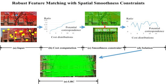
2.1. Workflow
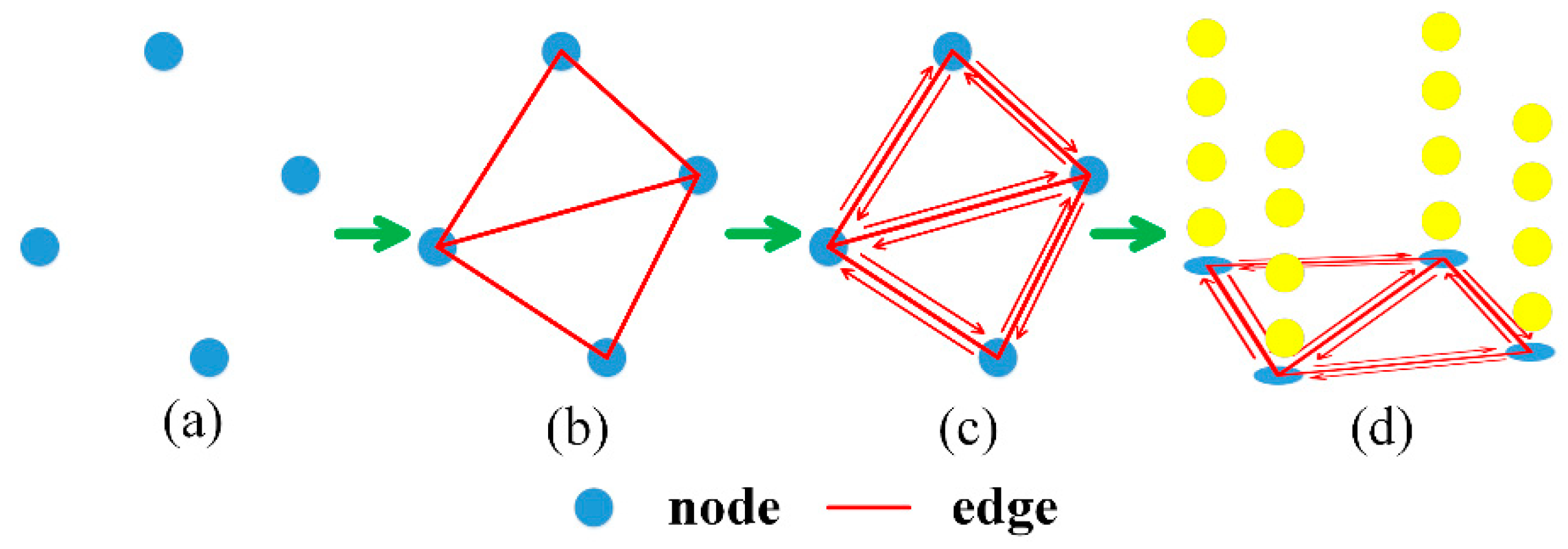
2.2. Feature Point Graph
2.3. Graph-Based Energy Function
2.4. Solution
| Algorithm 1: The iterative solution of the sub-optimization in the proposed method |
| Function: Iterative_solution_of_sub_optimizations (PB, POther, , , ) Input: the set of feature point in the basic image PB, the set of feature point in the other image POther, the set of connected points for each feature point in the basic image ; the set of matching cost of all feature point C; Output: the set of matching results of all feature points in the basic image |
Pseudo-code:
|
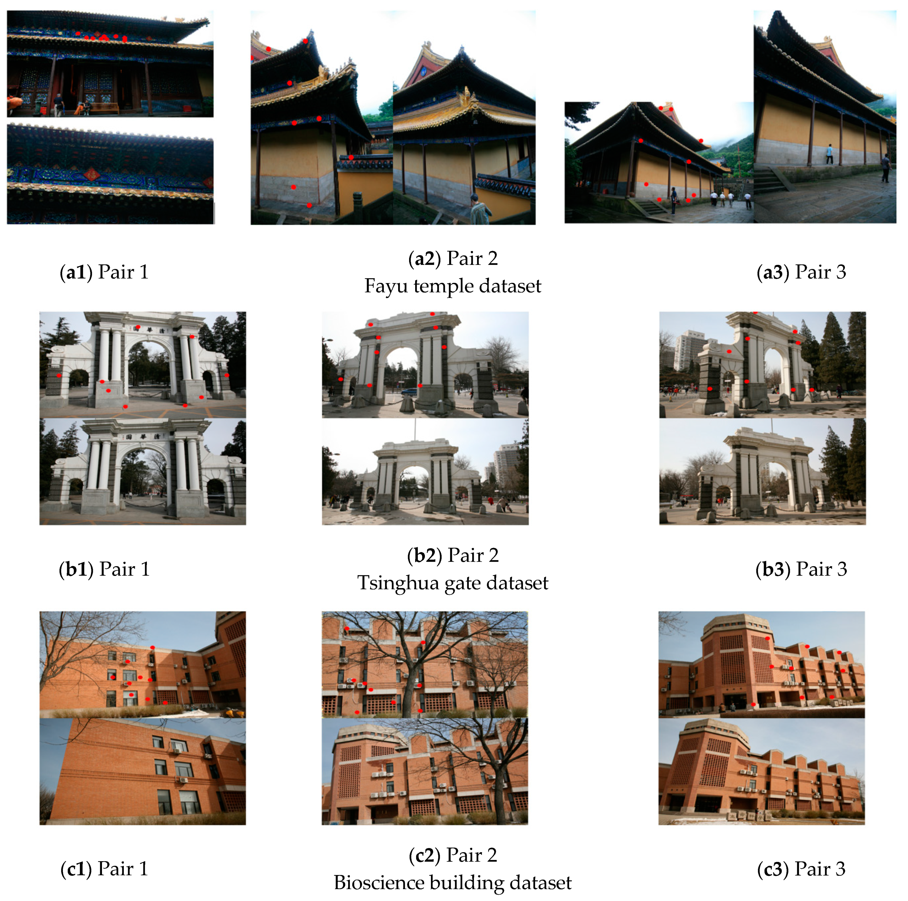
3. Study Areas and Data
4. Results
4.1. Analysis about the Influence of the Number of the Potential Correspondences on the Final Matching Results
4.2. Analysis about the Influence of the Initial Penalty Coefficient on the Final Matching Results
4.3. Matching Accuracy Comparisons on More Datasets
5. Discussion
6. Conclusions
Author Contributions
Funding
Acknowledgments
Conflicts of Interest
References
- Szeliski, R. Computer Vision: Algorithms and Applications, 1st ed.; Springer: Berlin, Germany, 2010; pp. 183–228. [Google Scholar]
- Ling, X.; Huang, X.; Zhang, Y.; Zhou, G. Matching Confidence Constrained Bundle Adjustment for Multi-View High-Resolution Satellite Images. Remote Sens. 2020, 12, 20. [Google Scholar] [CrossRef] [Green Version]
- Huang, X.; Liu, W.; Qin, R. A window size selection network for stereo dense image matching. Int. J. Remote Sens. 2020, 41, 4836–4846. [Google Scholar] [CrossRef]
- Huang, X.; Hu, K.; Ling, X.; Zhang, Y.; Lu, Z.; Zhou, G. Global Patch Matching. In Proceedings of the ISPRS Annals of the Photogrammetry, Remote Sensing and Spatial Information Sciences, Wuhan, China, 18–22 September 2017; pp. 227–234. [Google Scholar]
- Liu, X.; Zhang, Y.; Ling, X.; Wan, Y.; Liu, L.; Li, Q. TopoLAP: Topology Recovery for Building Reconstruction by Deducing the Relationships between Linear and Planar Primitives. Remote Sens. 2019, 11, 1372. [Google Scholar] [CrossRef] [Green Version]
- Ren, Z.; Meng, J.; Yuan, J. Depth camera based hand gesture recognition and its applications in Human-Computer-Interaction. In Proceedings of the International Conference on Information and Communication Security, Singapore, 13–16 December 2011; pp. 1–5. [Google Scholar]
- Kim, Y.; Baek, S.; Bae, B. Motion Capture of the Human Body Using Multiple Depth Sensors. ETRI J. 2017, 39, 181–190. [Google Scholar] [CrossRef]
- Kim, K.; Lawrence, R.L.; Kyllonen, N.; Ludewig, P.M.; Ellingson, A.M.; Keefe, D.F. Anatomical 2D/3D shape-matching in virtual reality: A user interface for quantifying joint kinematics with radiographic imaging. In Proceedings of the IEEE Symposium on 3d User Interfaces, Los Angeles, CA, USA, 18–19 March 2017; pp. 243–244. [Google Scholar]
- Kim, J.; Lin, S.; Hong, J.; Kim, Y.; Park, C. Implementation of Martian virtual reality environment using very high-resolution stereo topographic data. Comput. Geosci. 2012, 44, 184–195. [Google Scholar] [CrossRef]
- Wu, Y.; Di, L.; Ming, Y.; Lv, H.; Tan, H. High-Resolution Optical Remote Sensing Image Registration via Reweighted Random Walk based Hyper-Graph Matching. Remote Sens. 2019, 11, 2841. [Google Scholar] [CrossRef] [Green Version]
- Yang, H.; Li, X.; Zhao, L.; Chen, S. A Novel Coarse-to-Fine Scheme for Remote Sensing Image Registration Based on SIFT and Phase Correlation. Remote Sens. 2019, 11, 1833. [Google Scholar] [CrossRef] [Green Version]
- Wang, M.; Zhang, H.; Sun, W.; Li, S.; Wang, F.; Yang, G. A Coarse-to-Fine Deep Learning Based Land Use Change Detection Method for High-Resolution Remote Sensing Images. Remote Sens. 2020, 12, 1933. [Google Scholar] [CrossRef]
- Dong, H.; Ma, W.; Wu, Y.; Zhang, J.; Jiao, L. Self-Supervised Representation Learning for Remote Sensing Image Change Detection Based on Temporal Prediction. Remote Sens. 2020, 12, 1868. [Google Scholar] [CrossRef]
- He, F.; Zhou, T.; Xiong, W.; Hasheminnasab, S.M.; Habib, A. Automated Aerial Triangulation for UAV-Based Mapping. Remote Sens. 2018, 10, 1952. [Google Scholar] [CrossRef] [Green Version]
- Iacobucci, G.; Troiani, F.; Milli, S.; Mazzanti, P.; Piacentini, D.; Zocchi, M.; Nadali, D. Combining Satellite Multispectral Imagery and Topographic Data for the Detection and Mapping of Fluvial Avulsion Processes in Lowland Areas. Remote Sens. 2020, 12, 2243. [Google Scholar] [CrossRef]
- Wan, Y.; Zhang, Y.; Liu, X. An a-contrario method of mismatch detection for two-view pushbroom satellite images. ISPRS J. Photogramm. Remote Sens. 2019, 153, 123–136. [Google Scholar] [CrossRef]
- Wan, Y.; Zhang, Y. The P2L method of mismatch detection for push broom high-resolution satellite images. ISPRS J. Photogramm. Remote Sens. 2017, 130, 317–328. [Google Scholar] [CrossRef]
- Huang, X.; Qin, R. Multi-view large-scale bundle adjustment method for high-resolution satellite images. In Proceedings of the ASPRS Conference, Denver, CO, USA, 27–31 January 2019. [Google Scholar]
- Tatar, N.; Arefi, H. Stereo rectification of pushbroom satellite images by robustly estimating the fundamental matrix. Int. J. Remote Sens. 2019, 40, 8879–8898. [Google Scholar] [CrossRef]
- Qin, R. RPC Stereo Processor (RSP): A Software Package for Digital Surface Model and Orthophoto Generation from Satellite Stereo Imagery. In Proceedings of the ISPRS Annals of the Photogrammetry, Remote Sensing and Spatial Information Sciences, Prague, Czechoslovakia, 12–19 July 2016; pp. 77–82. [Google Scholar]
- Jiang, S.; Jiang, W. On-Board GNSS/IMU Assisted Feature Extraction and Matching for Oblique UAV Images. Remote Sens. 2017, 9, 813. [Google Scholar] [CrossRef] [Green Version]
- Hu, H.; Zhu, Q.; Du, Z.; Zhang, Y.; Ding, Y. Reliable Spatial Relationship Constrained Feature Point Matching of Oblique Aerial Images. Photogramm. Eng. Remote Sens. 2015, 81, 49–58. [Google Scholar] [CrossRef]
- Zhang, Y.; Xiong, X.; Zheng, M.; Huang, X. LiDAR Strip Adjustment Using Multifeatures Matched with Aerial Images. IEEE T. Geosci. Remote Sens. 2015, 53, 976–987. [Google Scholar] [CrossRef]
- Ling, X.; Zhang, Y.; Xiong, J.; Huang, X.; Chen, Z. An Image Matching Algorithm Integrating Global SRTM and Image Segmentation for Multi-Source Satellite Imagery. Remote Sens. 2016, 8, 672. [Google Scholar] [CrossRef] [Green Version]
- Duan, Y.; Huang, X.; Xiong, J.; Zhang, Y.; Wang, B. A combined image matching method for Chinese optical satellite imagery. Int. J. Digit. Earth 2016, 9, 851–872. [Google Scholar] [CrossRef]
- Lowe, D.G. Distinctive Image Features from Scale-Invariant Keypoints. Int. J. Comput. Vis. 2004, 60, 91–110. [Google Scholar] [CrossRef]
- Bay, H.; Tuytelaars, T.; Van Gool, L. SURF: Speeded up robust features. In Proceedings of the European Conference on Computer Vision, Graz, Austria, 12–18 October 2006; pp. 404–417. [Google Scholar]
- Leutenegger, S.; Chli, M.; Siegwart, R. BRISK: Binary Robust invariant scalable keypoints. In Proceedings of the International Conference on Computer Vision, Barcelona, Spain, 6–13 November 2011; pp. 2548–2555. [Google Scholar]
- Morel, J.; Yu, G. ASIFT: A New Framework for Fully Affine Invariant Image Comparison. SIAM J. Imag. Sci. 2009, 2, 438–469. [Google Scholar] [CrossRef]
- Fern, P.; Alcantarilla, N.; Bartoli, A.; Davison, A.J. KAZE features. In Proceedings of the European Conference on Computer Vision, Florence, Italy, 7–13 October 2012; pp. 214–227. [Google Scholar]
- Sons, M.; Kinzig, C.; Zanker, D.; Stiller, C. An Approach for CNN-Based Feature Matching Towards Real-Time SLAM. In Proceedings of the International Conference on Intelligent Transportation Systems, Auckland, New Zealand, 27–30 October 2019; pp. 1305–1310. [Google Scholar]
- Zagoruyko, S.; Komodakis, N. Learning to compare image patches via convolutional neural networks. In Proceedings of the Computer Vision and Pattern Recognition, Boston, MA, USA, 7–12 June 2015; pp. 4353–4361. [Google Scholar]
- Li, J.; Hu, Q.; Ai, M. 4FP-Structure: A Robust Local Region Feature Descriptor. Photogramm. Eng. Remote Sens. 2017, 83, 813–826. [Google Scholar] [CrossRef]
- Chen, M.; Qin, R.; He, H.; Zhu, Q.; Wang, X. A Local Distinctive Features Matching Method for Remote Sensing Images with Repetitive Patterns. Photogramm. Eng. Remote Sens. 2018, 84, 513–524. [Google Scholar] [CrossRef]
- Ma, J.; Zhao, J.; Tian, J.; Yuille, A.L.; Tu, Z. Robust point matching via vector field consensus. IEEE Trans. Imag. Process. 2014, 23, 1706–1721. [Google Scholar] [CrossRef] [Green Version]
- Winter, M.; Ober, S.; Arth, C.; Bischof, H. Vocabulary Tree Hypotheses and Co-Occurrences. In Proceedings of the 12th Computer Vision Winter Workshop (CVWW’07), St. Lambrecht, Austria, 6–8 February 2007. [Google Scholar]
- Shewchuk, J.R. Triangle: Engineering a 2D quality mesh generator and Delaunay triangulator. In Proceedings of the Workshop on Applied Computational Geometry, Philadelphia, PA, USA, 27–28 May 1996; pp. 203–222. [Google Scholar]
- Zhou, K.; Hou, Q.; Wang, R.; Guo, B. Real-time Kd-tree Construction on Graphics Hardware. ACM Trans. Graph. 2008, 27, 1–11. [Google Scholar]
- 3D Reconstruction Dataset. Available online: http://vision.ia.ac.cn/data (accessed on 19 August 2020).
- Fischler, M.A.; Bolles, R.C. Random sample consensus: A paradigm for model fitting with applications to image analysis and automated cartography. Commun. ACM 1981, 24, 381–395. [Google Scholar] [CrossRef]


© 2020 by the authors. Licensee MDPI, Basel, Switzerland. This article is an open access article distributed under the terms and conditions of the Creative Commons Attribution (CC BY) license (http://creativecommons.org/licenses/by/4.0/).
Share and Cite
Huang, X.; Wan, X.; Peng, D. Robust Feature Matching with Spatial Smoothness Constraints. Remote Sens. 2020, 12, 3158. https://doi.org/10.3390/rs12193158
Huang X, Wan X, Peng D. Robust Feature Matching with Spatial Smoothness Constraints. Remote Sensing. 2020; 12(19):3158. https://doi.org/10.3390/rs12193158
Chicago/Turabian StyleHuang, Xu, Xue Wan, and Daifeng Peng. 2020. "Robust Feature Matching with Spatial Smoothness Constraints" Remote Sensing 12, no. 19: 3158. https://doi.org/10.3390/rs12193158