Comparison of Empirical and Physical Modelling for Estimation of Biochemical and Biophysical Vegetation Properties: Field Scale Analysis across an Arctic Bioclimatic Gradient

Abstract

To evaluate the potential of multi-angle hyperspectral sensors for monitoring vegetation variables in Arctic environments, empirical and physical modelling using field data was implemented for the retrieval of leaf and canopy chlorophyll content (LCC, CCC) and plant area index (PAI) measured at four sites situated across a bioclimatic gradient in the Western Canadian Arctic. Field reflectance data were acquired with an ASD FieldSpec (305–1075 nm) and used to simulate CHRIS Mode1 spectra (411–997 nm). Multi-angle measurements were taken corresponding to CHRIS view zenith angles (VZA) (−55°, −36°, 0°, +36°, +55°). Empirical modelling compared parametric regression based on vegetation indices (VIs) to non-parametric Gaussian Processes Regression (GPR). In physical modelling, PROSAIL was inverted using numerical optimization and look-up table (LUT) approaches. Cross-validation of the empirical models ranked GPR as best, followed by simple ratio (SR) with optimally selected NIR and red wavelengths, and then ROSAVI using its published wavelengths (mean r²_cv = 0.62, 0.58, and 0.54, respectively across all sites, variables, and VZAs). However, the best predictive performance was achieved by SR followed by GPR and ROSAVI (NRMSE_cv = 0.12, 0.16, 0.16, respectively). PROSAIL simulated the multi-angle top-of-canopy reflectance well with numerical optimization (r² = ~0.99, RMSE = 0.004 ± 0.002), but best performing LUT models of LCC, CCC and PAI were poorer than the empirical approaches (mean r² = 0.48, mean NRMSE = 0.22). PROSAIL performed best at the high Arctic sparsely vegetated site (r² = 0.57–0.86 for all parameters). Overall, the best performing VZA was −55° for empirical modelling and 0° and ±55° for physical modelling; however, these were not significantly better than the other VZAs. Overall, this study demonstrates that, for Arctic vegetation, nadir narrowband reflectance data used to derive simple empirical VIs with optimally selected bands is a more efficient approach for modelling chlorophyll and PAI than more complex empirical and physical approaches.

1. Introduction

Estimation and mapping of vegetation biophysical and biochemical characteristics is one of the most common applications of optical remote sensing and is implemented at all scales from local to global. Quantifying biochemical constituents is of great interest because of their importance to foliar and ecosystem processes (e.g., photosynthesis and nutrient cycling), their use for identifying plant functional groups based on differences in leaf/canopy traits, and their use for assessing plant and ecosystem stress (e.g., water stress) [1,2,3]. Quantification of biophysical characteristics can provide a means of characterizing the structural aspects of vegetation canopies (e.g., plant area index, PAI), scaling up foliar biochemical measurements to the canopy scale, understanding dynamic changes to ecosystem phenology and productivity (e.g., biomass), and be used as an indicator for climate related impacts on ecosystems (e.g., the assessment of trends related to greening/browning) [4,5,6]. Accurate remotely sensed estimates of both vegetation biochemical and biophysical characteristics provide a valuable aid to understanding ecosystem composition and its functioning over a wide range of environments and spatio-temporal scales [3]. The retrieval of plant variables/traits are therefore especially valuable in understanding Arctic ecosystems where the cumulative effects of changing Arctic vegetation on the climate system in response to recent warming and the relative importance of competing feedbacks related to tundra vegetation (e.g., albedo, photosynthetic, and respiratory processes), are still not well known [7,8,9,10]. This is primarily due to the size and remoteness of the Arctic, its diversity of ecosystems and vegetation, and the biomass quantities involved [11,12].

Recent and near future high spatial and spectral resolution airborne and satellite sensors (e.g., hyperspectral or spectroscopic sensors) such as AVIRIS-NG (Airborne Visible Infrared Imaging Spectrometer—Next Generation) [13], PRISMA (Hyperspectral Precursor and Application Mission) [14], and EnMAP (Environmental Mapping and Analysis Program) [15] are enabling enhanced retrieval capabilities for monitoring plant variables, such as pigment biochemistry (e.g., chlorophyll, carotenoid, and anthocyanin content), non-pigment biochemistry (e.g., nitrogen, lignin, and cellulose) and canopy biophysical attributes (e.g., PAI) [1,2,16,17,18,19,20,21,22]. In addition, multi-angle spectroscopic sensors, such as CHRIS/PROBA [23], provide valuable spectral data for testing and validating the angular properties of reflectance models [5,6]. Despite these benefits, increasing spectral data dimensionality and data volumes require enhanced and robust retrieval techniques. Imaging spectroscopy data often contain highly correlated and noisy spectral bands that can affect prediction/retrieval accuracy [24,25,26]. Selection of the best predictor variables from a feature-rich dataset is necessary for the selection of the optimal predictive model.

Vegetation modelling using imaging spectroscopy data is typically conducted using empirical or physically based methods. Empirical methods (both parametric and non-parametric) have been shown to produce excellent results in a variety of environments [27,28,29], while providing a rather simple and straightforward approach for implementation. Studies using parametric regression have shown that strong relationships can be developed between spectral predictor variables (e.g., vegetation indices, VIs) and a variable of interest [5,6,29,30,31]; however, these methods may not yield optimal results when datasets are complex and non-linear [24,30,32]. In contrast, non-parametric approaches (e.g., machine learning regression algorithms, MLRAs) exploit the full reflectance signal and are capable of modelling non-linear relationships [24,30,32]. Non-parametric approaches have been shown to work well with highly dimensional, multicollinear spectroscopic data and have been shown to outperform linear parametric regression based on VIs [24,30,32]. Two limitations related to their use are: (1) parameterized empirical models may not be transferrable to new locations and sensors as they typically require recalibration, and (2) empirical models can suffer from statistical problems such as overfitting [30]. In comparison, physical radiative transfer models (RTMs) describe the interaction (absorption, scattering and reflectance) of radiation within a medium, typically leaves and their associated canopies, using physical laws and are thus considered generalizable across ecosystems [33]. Leaf and canopy RTMs, such as PROSAIL [PROSPECT (leaf properties) + SAIL (canopy properties)] [34,35,36,37], assume that radiative transfer and interaction of radiation within leaves and canopies is a function of leaf structure and biochemistry, canopy architecture/configuration, and soil characteristics (e.g., moisture and composition) [34,38,39]. RTMs therefore provide an explicit link between vegetation biophysical and biochemical variables and canopy reflectance [33]. Furthermore, RTMs do not require significant calibration datasets and allow for all spectral information to be used simultaneously [38]. A disadvantage to their implementation is that the inversion of RTMs is mostly ill-posed [33,40,41,42]; various combinations of input parameters can result in the same solution.

In the Arctic, empirical vegetation modelling (e.g., biophysical variable estimation and retrieval) has mostly been conducted using field spectral reflectance measurements [29,31,43,44,45,46,47,48,49,50,51,52]. The conclusions of these studies are typically recommendations for a set of meaningful narrow spectral bands used to map the variable in question. For example, Bratsch et al. [43] used partial least squares regression (PLSR) to identify optimal spectral bands for classifying four Alaskan vegetation types. Currently, no studies have measured foliar biochemical quantities in the field (e.g., chlorophyll) for remote sensing retrieval purposes, and furthermore, there has not been a robust comparison of spectroscopic-based retrieval methods or analyses of multi-angle spectral information using either empirical or physical modelling approaches. The use and adoption of MLRAs and deep learning algorithms has increased substantially within the remote sensing community [30,53]; however, their implementation in tundra environments is also largely missing from the literature. Studies examining machine learning regression algorithms have demonstrated that Gaussian processes regression (GPR) [54] achieves high performances and is capable of outperforming other machine learning approaches for the retrieval of vegetation biochemical and biophysical variables from field, airborne, and satellite imaging spectroscopy data [24,32,55,56]. GPR is a non-parametric, Bayesian MLRA that is capable of providing statistical descriptions of the predicted variables, such as variable rankings and uncertainty measures [24,54]. Recently, Wang et al. [57] compared GPR to PLSR for retrieving 15 foliar functional traits in a grassland ecosystem from AVIRIS data. Results showed that GPR and PLSR performed comparably with respect to predictions and spectral variable selection. Although GPR has been used in these experimental studies, it has not been fully tested across environments and spectroscopic sensors and remains to be tested for predicting leaf and canopy biophysical and biochemical parameters in Arctic environments.

Physical models have had very limited testing in Arctic environments [58], including the evaluation of various cost functions and regularization approaches [59]. PROSAIL has seen widespread adoption and increasing use in a variety of environments [38], including sparse/short vegetation ecosystems with spatially heterogeneous plant assemblages, such as grasslands and chaparral ecosystems that are comparable to Arctic tundra. For example, Darvishzadeh et al. [20] inverted the PROSAIL model in order to estimate vegetation leaf area index (LAI) and chlorophyll in a heterogeneous grassland. Results of their study showed that canopy chlorophyll content could be retrieved with accuracies similar to empirical approaches (e.g., r²=0.70, NRMSE=0.18) and that stratification of field data based on species heterogeneity was an important consideration. In a secondary study in the same ecosystem, Darvishzadeh et al. [21] showed that LAI can be estimated with PROSAIL with high accuracies up to (r²= 0.91, NRMSE = 0.18) when wavebands not well simulated by PROSAIL were discarded. Zarco-Tejada et al. [60] inverted the PROSAIL model for the estimation of leaf equivalent water thickness from Moderate Resolution Imaging Spectroradiometer (MODIS) reflectance data in dry, shrubby chaparral ecosystems. Results showed a high correlation between measured and estimated leaf moisture (e.g., r² = 0.70). Hilker et al. [61] showed that PROSAIL is able to accurately predict chlorophyll concentrations using multi-angle, multi-temporal MODIS data in Amazon ecosystems at regional scales (e.g., r² = 0.73–0.98). Casas et al. [62] used PROSAIL to estimate water related biophysical and biochemical variables (e.g., LAI) using multitemporal AVIRIS data in a spatially heterogeneous Mediterranean ecosystem (e.g., forest, grasses, shrubs). The study showed good performance in grasses and shrubs when a known soil spectrum was incorporated into the RTM. Furthermore, the PROSAIL model has been previously used to estimate biophysical and biochemical attributes of natural canopies as it relates to multi-angle reflectance data [63]. Although PROSAIL is a canopy model with simplified assumptions of canopy structure (i.e., it is defined as a one-dimensional turbid medium model that simplifies the canopy into an idealized mixture), this should not invalidate its use in natural ecosystems [33], especially when the spatial heterogeneity of the ecosystem can be accounted for within the sampling design (i.e., the scale of the elements are sufficiently accounted for relative to the spatial scale of the sensor spatial resolution). The use of physical modelling (PROSAIL) and the testing of various inversion procedures (including cost functions, multiple best solutions, and parameter/spectral noise) provide an innovative approach to this study as there is limited to no studies that have investigated these methods for estimating tundra plant biochemical and biophysical parameters from multi-angle, spectroscopic data.

Multi-angle imaging spectroscopy, or spectrodirectional remote sensing, is defined as the near-simultaneous acquisition of spatially co-registered images in many spectrally contiguous bands, at various observation and illumination angles [64,65]. Spectrodirectional observations have been shown to significantly improve the quality and reliability of reflectance-based vegetation variable/trait estimates [5,6,64,66,67,68], but have not been extensively investigated for this purpose in Arctic environments. Vierling et al. [69], using in situ spectrodirectional data, showed that larger VI differences exist in the forward scatter direction than in the backscatter direction and VI differences are significantly more pronounced at progressively larger solar zenith angles. In the same study, Vierling et al. [69] showed that off-nadir spectral measurements can be used to discriminate between tussock tundra sites possessing varying degrees of woody materials and may be useful for detecting these changes through time. These results suggest that there is a need to account for the directional effects over the Arctic due to the extreme sun/sensor angles, given that non-nadir views typically provide different fractions of viewed shade/sunlit canopy and background (e.g., soil contributions). Buchhorn et al. [70] showed that normalized difference vegetation index (NDVI) and biomass estimates in Arctic tundra ecosystems are influenced by sun-object-sensor geometries (i.e., bidirectional reflectance distribution function effects), and that these effects are more pronounced over the irregular/rough surfaces and extreme sun-sensor geometries. It is evident from the literature that there is a general lack of testing across Arctic environments using both empirical and physical techniques to estimate biochemical and biophysical constituents from multi-angular remote sensing data.

In this paper, Arctic vegetation modelling of chlorophyll and plant area index is presented as a comparison of parametric and non-parametric machine learning empirical methods to the PROSAIL RTM approach. This study was conducted using field data to provide reference information for the development of a follow-on study using the CHRIS/PROBA multi-angle hyperspectral sensor [71]; consequently, the scaling of field data from field to satellite scales (in both spatial and spectral domains) was considered an important component of this investigation. The objectives were to:

• compare multi-angle vegetation spectra and measurements of leaf and canopy chlorophyll (LCC, CCC, respectively) and plant area index (PAI) at various locations in the Western Canadian Arctic that represent a latitudinal climate gradient;
• compare parametric linear regression combined with common VIs to non-linear non-parametric machine learning (GPR) for estimation of LCC, PAI, and CCC at all view angles and sites;
• compare the empirical modelling results to PROSAIL models inverted by LM and LUT methods;
• assess the effect of resampling spectral resolution and scaling-up field measurements on model results.

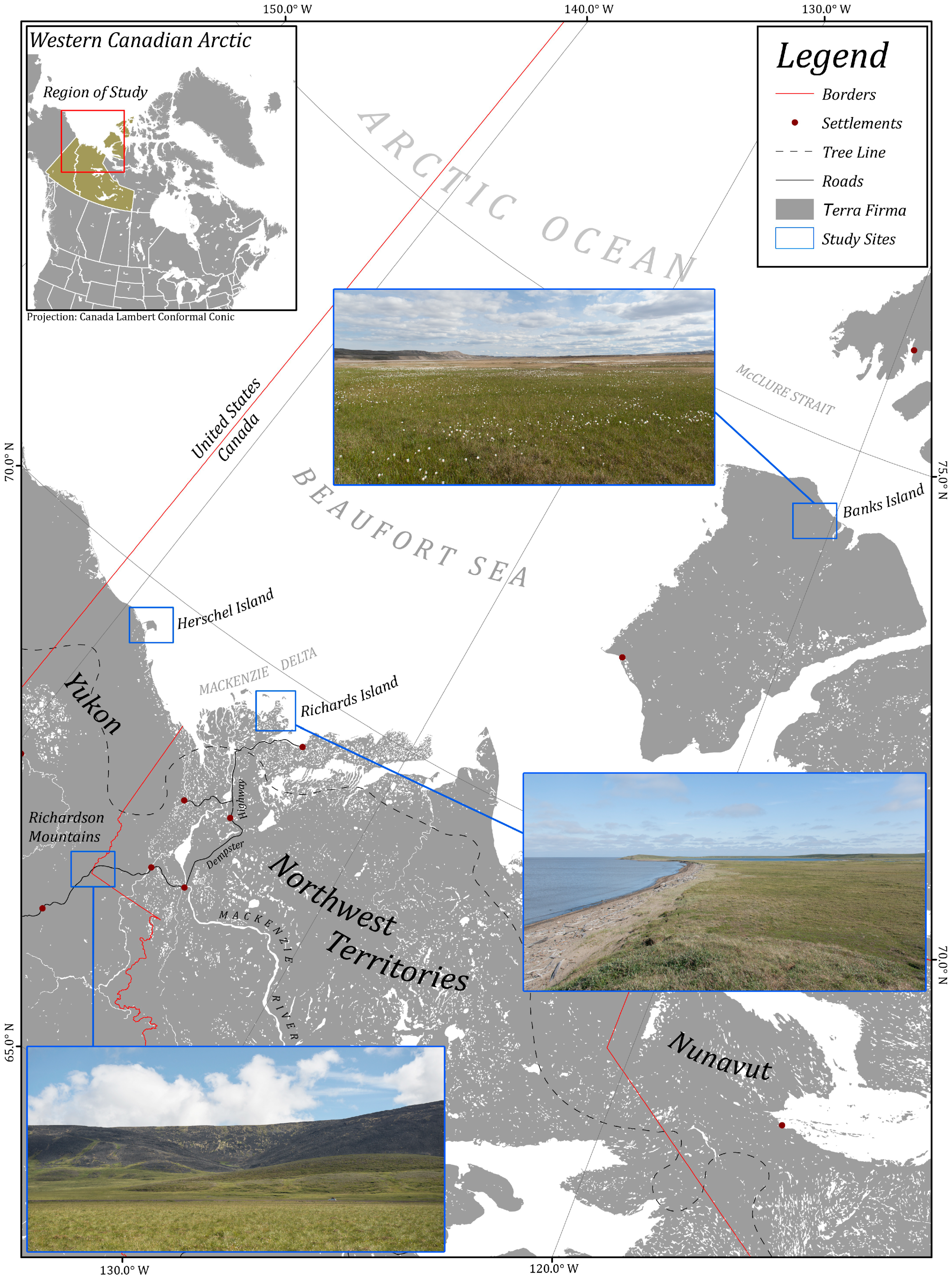
2. Study Sites

The study sites included Herschel Island (Yukon), Banks Island (Northwest Territories), Richards Island (Northwest Territories), and the Richardson Mountains (Yukon/Northwest Territories) (Figure 1). They are situated in the Northern and Southern Arctic and Taiga Cordillera Terrestrial Ecozones [72] within the Western Canadian Arctic. Satellite and historical records in the region, such as ground-based photographs and plot-based studies, provide evidence of enhanced greening [7,10,73,74,75,76,77,78,79,80,81] and rapid warming [82,83,84]. Changes to vegetation across this region may indicate how and how quickly other Arctic terrestrial ecosystems will respond to similar warming conditions [10]. Therefore, this region provides an ideal setting for vegetation related monitoring studies and methodological investigations.

Vegetation at the sites was comprised of herbaceous plants, prostrate and erect shrubs, mosses, sedges and grasses, and lichens [11,80]. The dominant species were: Vaccinium vitis-idaea var. minus (lingonberry), Arctostaphylos uva-ursi (bearberry), Vaccinium uliginosum (blueberry), Rubus chamaemorus (cloudberry), Petasites frigidus var. frigidus (Arctic sweet coltsfoot), Carex aquatilis (water sedge), Eriophorum vaginatum (cotton grass), Betula nana (dwarf birch), Salix pulchra (tealeaf willow), Rhododendron tomentosum (northern Labrador tea), Sphagnum (peat moss), and Empetrum nigrum (crowberry). Vegetation patterns across this Arctic region are strongly influenced by the presence of the Arctic ocean and its seasonal sea ice patterns [73,80]. Thus, the sites exhibited a general gradient from warmer with higher vegetation percent cover and diversity in the south (Richardson Mountains) to cooler with sparse vegetation in the north (Banks Island) [80,87,88]. Local landscape variations due to moisture, geology, soils, topography and permafrost features are also factors affecting vegetation species distribution and percent cover [80,89,90].

3. Methods

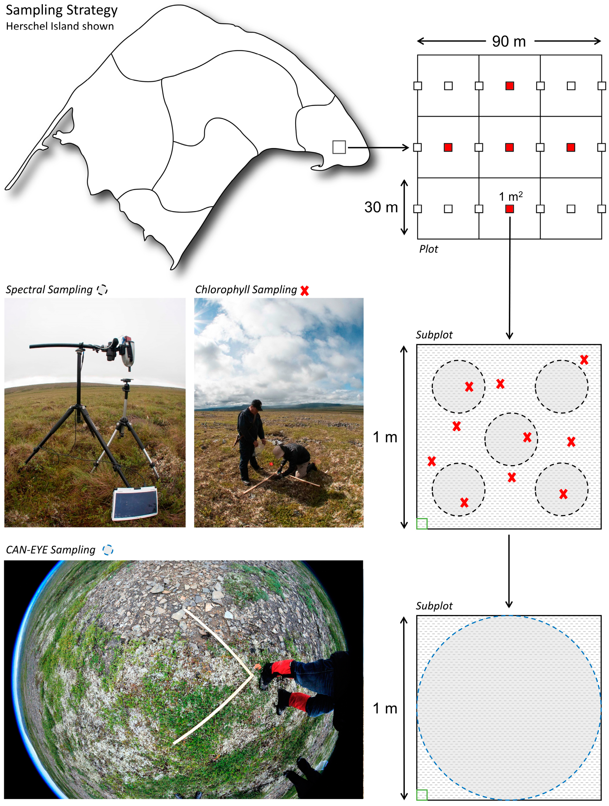
3.1. Field Sampling Design

All field sites were visited between July 10th and August 4th in the years between 2011 and 2014 during the peak of the growing season. Data were acquired in both 2013 and 2014 for the Richardson Mountains site.

Sampling for field measurements at each site was conducted following the design schematic shown in Figure 2. Between 18 and 33 plots of 90 m × 90 m were sampled at each site depending on accessibility and weather. This plot size was selected to represent approximately 3 × 3 pixels in CHRIS Mode 1 (M1) (34 m pixels at nadir) imagery [91] and to account for vegetation heterogeneity and adjacency effects within satellite imagery. Locations of plots were determined using a stratified sampling approach: spectrally distinct and uniformly vegetated areas were identified through visual analysis of moderate resolution imagery (Landsat 5 and 8) and through on-the-ground surveys. Within these zones, field plot locations were randomly selected away from edges and distinct gradients. The central location of each 30 m × 30 m square in Figure 2 was recorded with a handheld Trimble Juno GPS unit accurate to ~3 m. Subplots of 1 m × 1 m were placed within each plot as shown in Figure 2 (upper right). Within each subplot, five locations were selected for multi-angle spectral reflectance measurements (Figure 2, bottom right, dotted circles) and ten locations were randomly selected for destructive and non-destructive chlorophyll measurements (Figure 2, bottom right, red x’s). A downward hemispherical photo was taken in each subplot for estimation of PAI [92,93] and destructive vegetation samples were taken for lab measurement of PAI from the five red subplots in Figure 2.

3.2. Field Measurements of Leaf Chlorophyll Content (LCC)

Measurements of non-senescent LCC (µg/cm²) for the dominant species were made at each study site using a Minolta SPAD-502 chlorophyll meter (Minolta Camera Co. Osaka, Japan). Leaves were sampled randomly throughout the canopy and were sampled regardless of phenological state (both green and senescent leaves were included in the samples). The emphasis, however, was on sampling leaves (and other vegetation components) that would be detected by the optical sensor (i.e., leaves obscured from 90% of the canopy were not the primary sampling target), and so in this case, leaves occurring at the bottom of the canopy were not sampled. Species with extremely small needles were not sampled, as the SPAD field of view was too large for proper measurement. This instrument is commonly used to characterize chlorophyll concentration in plant species [19,20,21,94,95,96,97,98,99]. SPAD values are a unitless measure of LCC derived from transmittance in the red (650 nm) and near-infrared (NIR) (940 nm) using a calibrated light source [100]. Anatomical/morphological differences between specimens can confound readings, so caution should be exercised [91]. A predefined linear calibration function, or consensus equation [95], was used to convert the SPAD values to actual measurements of chlorophyll in µg/cm². Within each of the subplots, 10 SPAD readings (e.g., at red x’s in Figure 2) were averaged to produce one LCC measurement per subplot. To determine how well the SPAD measurements represented actual LCC values, lab-based measurements were made using destructive samples collected at the Richardson Mountains site. The lab-based methods for LCC, as well as carotenoids, non-pigments, equivalent water thickness (EWT), and leaf mass per area followed standard lab protocols (e.g., [101,102,103,104]). A full description of the lab-based procedures used to estimate these variables can be found in Kennedy [91]. The averaged pigment and non-pigment values for each species were then weighted by the species mass proportions in the plots to provide averaged values across the plot canopy. Using analysis of variance (ANOVA), no significant differences were found between the converted SPAD values and lab-derived LCC datasets, indicating that the converted SPAD (i.e., instrument-based measurements) LCC values for all sites could be used with confidence.

3.3. Field Measurements of PAI and Calculation of Canopy Leaf Chlorophyll Content (CCC)

Downward hemispherical photos (DHPs) were taken with a 12.3-megapixel Nikon D300 camera equipped with a Sigma 8 mm F3.5 EX DG Circular Fisheye lens. They were taken from an approximate height of 1.5 m at all subplot locations (white squares in Figure 2) for a total of 21 photos per plot to capture canopy spatial variability. Due to the limited time for this remote fieldwork, photographs were taken under all sky conditions and times of day. Photos were batch processed in Photoshop (Adobe Inc.) to correct white balance and exposure, and to partially eliminate shadowing, which varied between photos depending on sky conditions. Processing was limited to view zenith angles (VZA) equal to and less than 45° to limit the number of mixed pixels (at greater view angles) and limit the field of view to be just larger than the subplot size (i.e., 1 m²).

CAN-EYE software [105,106] was then used to derive PAI and average leaf inclination angle (ALA) (see Kennedy [91] for more details). PAI was used for this study because it considers all green vegetation components within the canopy (e.g., stems and leave) [58,92,106], whereas LAI, defined as the total surface area of green leaves relative to a defined ground surface area, does not capture/represent all photosynthetic components of tundra vegetation. Before processing, a calibration procedure was completed [106]. For each set of 21 DHPs per plot, gap fraction was calculated through two-class (vegetation, gap) supervised classification. Image classification was done in angular sectors with a zenith ($\Delta \theta$) resolution equal to 2.5° and an azimuth ($\Delta \phi$) resolution equal to 2.5°. Gap fraction ($P_{o, CAN-EYE}\left(\theta \right)$) was computed for each zenithal ring by taking the average values for all photographs across the 72 azimuthal sectors, excluding the masked areas. PAI was computed from the gap fraction using the Poisson law (distribution) as given in Welles and Norman [107] and Demarez et al. [108]. PAI values were calculated/integrated across transects and are therefore provided at the plot level.

To evaluate field CAN-EYE PAI values against a reference, the same Richardson Mountains site vegetation samples used for lab-based LCC measurement were laid out on a 1.8 m² white sheet in the lab and photographed (n = 99). Vegetation species such as moss may confound estimation of PAI due to its non-leafy structure and cover characteristics. Moss was not included in the destructive samples unless dominant and visibly exposed – only the top green components were harvested if present (i.e., the green components visible to the camera). Classification of vegetation was then conducted, and the relative number of vegetation pixels was taken as ‘destructive’ PAI [91]. Comparison of these to field-measured PAI values showed strong relationships with both ‘effective’ PAI (r² = 0.86, RMSE = 0.15), which does not account for clumping and ‘true’ PAI (r² = 0.77, RMSE = 0.21), which accounts for clumping. This gave confidence that the field PAI measurements for all sites were well representative and CAN-EYE derived effective PAI was selected for use in subsequent analyses.

Canopy chlorophyll content (CCC, g/m²) was then calculated by multiplying LCC by PAI. CCC has been used in other studies as a means of scaling up leaf-scale measurements and assessing canopy-level chlorophyll content [19,20,59,109,110]. It provides a more useful predictor of canopy chlorophyll than simply using LCC, since the spatial extent of vegetation cover is considered in the scaling.

Table 1. Descriptive statistics for: (1) converted and destructive LCC values (µg/cm²), (2) measured and destructive PAI values (dimensionless), and (3) measured and destructive CCC values (g/cm²) for all field sites. Plots with zero values excluded (no leaf measurements taken). Lab-based (spectrophotometric) LCC values are indicated with a superscript a. Destructive field-based values are denoted with a superscript b. Standard error (Std. Err.) was calculated by dividing the standard deviation by the square root of the sample size. LCC and CCC are displayed for the subplot scale (1 m²), whereas PAI values are shown for the plot scale (90 × 90 m).

LCC (µg/cm2)	Subplot
Field Site	n	Mean	Min	Max	Std. Err.
Herschel Island (2011)	693	34.9	19.0	54.8	0.2
Banks Island (2012)	520	32.0	12.6	49.5	0.3
Richards Island (2013)	162	33.5	19.0	53.1	0.5
Richardson Mountains (2013)	225	36.1	22.2	55.3	0.4
Richardson Mountains (2014 a)	360	37.5	3.8	65.9	0.8
Richardson Mountains (2014 b)	99	40.7	31.0	50.4	0.4
PAI (dimensionless)	Plot
Field Site	n	Mean	Min	Max	Std. Err.
Herschel Island (2011)	33	0.82	0.50	1.40	0.04
Banks Island (2012)	31	0.44	0.00	0.98	0.05
Richards Island (2013)	18	0.80	0.34	1.43	0.06
Richardson Mountains (2013)	25	1.09	0.61	1.50	0.04
Richardson Mountains (2014)	20	1.14	0.35	1.82	0.09
Richardson Mountains (2014 b)	20	1.18	0.35	1.74	0.09
CCC (g/m2)	Subplot
Field Site	n	Mean	Min	Max	Std. Err.
Herschel Island (2011)	693	0.29	0.06	0.89	0.01
Banks Island (2012)	520	0.18	0.01	0.65	0.00
Richards Island (2013)	162	0.27	0.05	0.90	0.01
Richardson Mountains (2013)	225	0.40	0.15	0.83	0.01
Richardson Mountains (2014)	99	0.47	0.11	0.80	0.02
Richardson Mountains (2014 b)	99	0.48	0.04	0.99	0.02

shows the descriptive statistics for LCC, PAI, and CCC measured at each field site. All variables showed a north–south gradient, where lowest overall values for each occurred at the Banks Island field site [91].

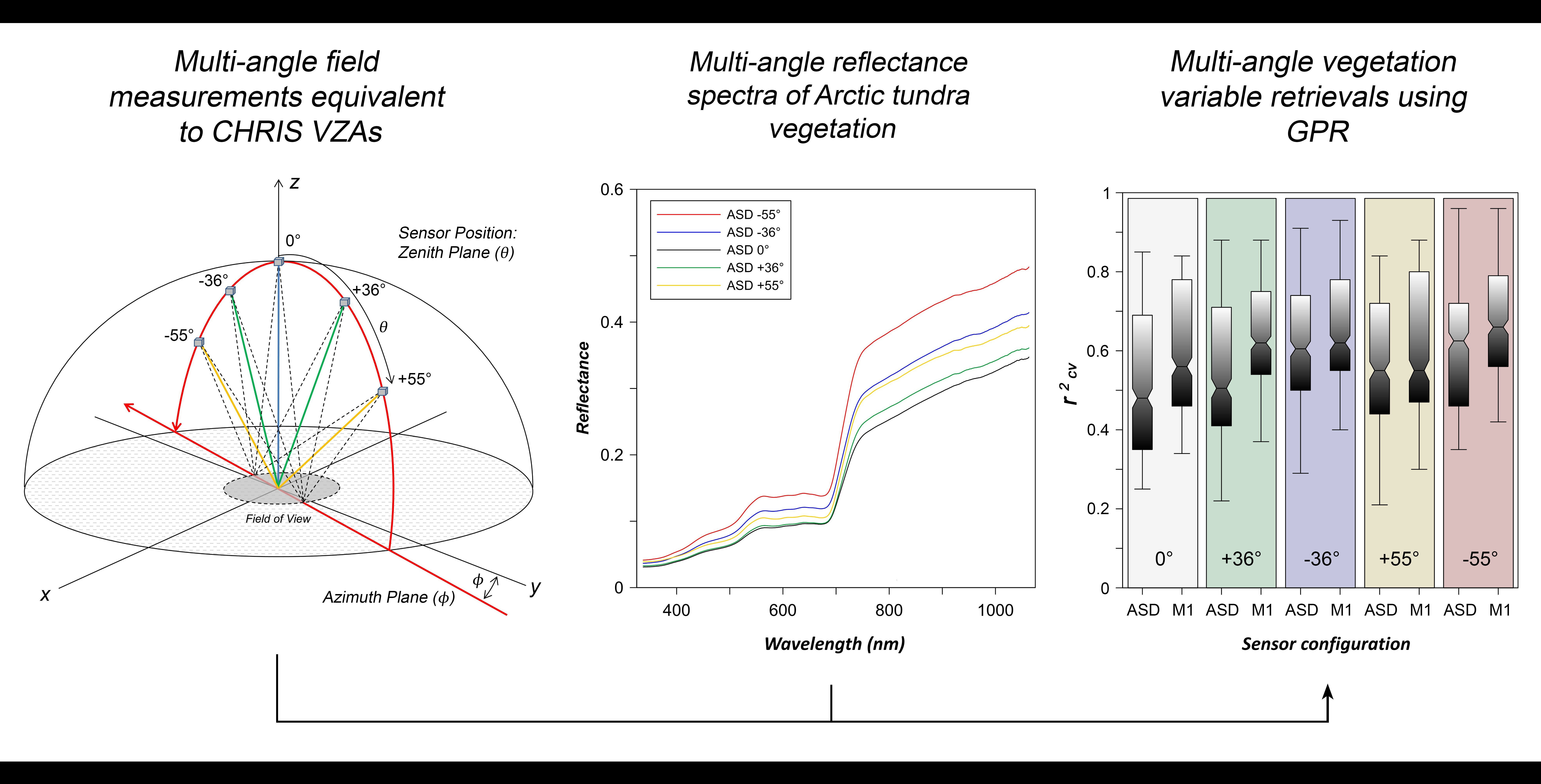
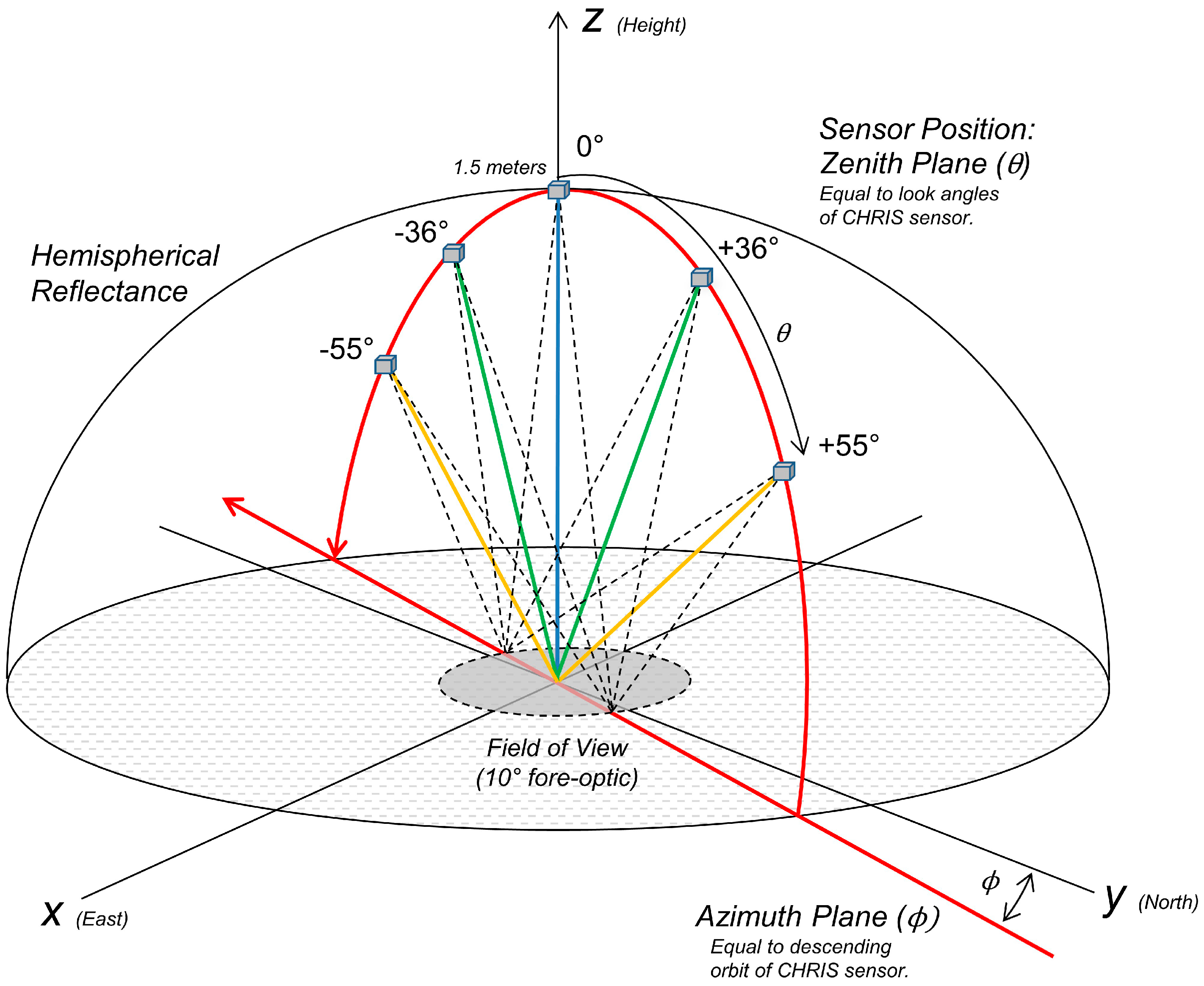
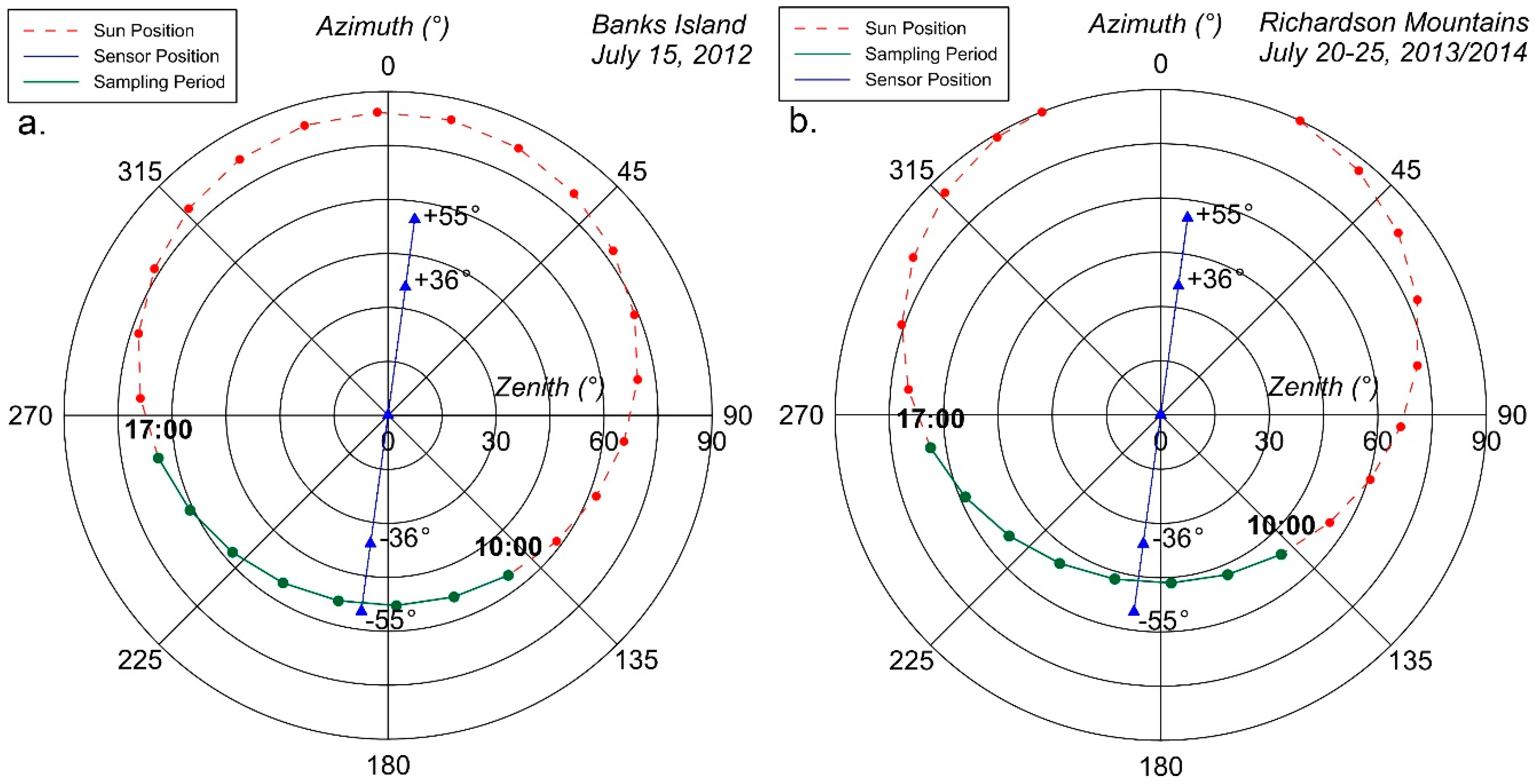
3.4. Field Spectral Reflectance Measurements and CHRIS/PROBA Simulation

Spectral reflectance measurements were acquired in each subplot (Figure 2) using an ASD FieldSpec handheld spectroradiometer (Analytical Spectral Devices, Inc. Boulder, USA) with a 10° fore optic. It uses a 512-channel silicon photodiode array, recording radiance between 305 nm and 1075 nm in 1.6 nm nominal bandwidths. Reflectance was derived by comparing radiance values to those for a Spectralon panel (Labsphere Inc., North Sutton, New Hampshire, USA). Measurements were taken at nadir, ±36° and ±55° (Figure 3), the VZAs of the CHRIS/PROBA sensor/platform, where positive angles correspond to forward scatter and negative angles to backscatter (see Kennedy et al. [71], which integrates the findings of this paper in vegetation modelling using multi-angle CHRIS M1 data). A tripod with fine angle adjustment was used and angles were measured using a digital inclinometer (accuracy ±0.2°) (Beall Tool Company, Newark, Ohio, USA) mounted on the spectroradiometer. Measurement height at nadir was 1.5 m and was reduced for ±36° and ±55° in an arc, similar to a goniometer. The resulting ground field of view (GFOV) varied from ~26 cm (nadir) to ~50 cm (±55°) but all GFOVs were less than one-half the subplot size. Furthermore, measurements were taken on the CHRIS/PROBA descending pathway angle of ~7.84° from true north to best simulate its expected VZA geometry. Timing of data acquisition was planned to align with CHRIS acquisitions, but this was not always possible due to weather and variable CHRIS/PROBA acquisition timing.

Five measurements taken at the same position in each subplot were averaged to a single subplot value. These 21 subplot values were then averaged to derive a single value for each 90 m × 90 m plot (Figure 2). In addition, subplot and plot averages were convolved to the 62 spectral bands (400–1050 nm; ~10 nm bandwidth) of CHRIS M1 data using the equation presented in [29,111]. A full description of the methodology used to simulate CHRIS data can be found in Kennedy [91]. All measured field spectra were filtered with the Savitzky-Golay [112] technique using a second order polynomial and 15 data points (i.e., wavelengths). This technique is widely used in spectroscopy [113] for noise reduction while preserving the higher order moments of the original spectrum. Overly noisy portions at both ends of the spectral range were discarded, resulting in spectra between 400 nm and 1050 nm for the ASD full spectrum data, and 411 nm to 997 nm for the simulated 62-band CHRIS M1 data.

Although a thorough analysis was not completed for the exact position/geometry of the sun in relation to the sensor, sampling at each site was completed at comparable seasons (mid-July) and daily times (~10:00 h to 17:00 h) to reduce inter-site sun-induced variability. The associated polar plots of the sun/sensor positions for the high-Arctic and low-Arctic sites can be seen in Figure 4 (sampling periods are shown in green; 24-hour sun positions are shown in red). Sun zenith angles (SZA) typically varied between ~46° to 66° and sun azimuth angles (SAA) varied from ~139° to 262° for all field sites, where greater SZAs occurred at lower latitudes (i.e., Richardson Mountains). Finally, ground spectra were taken to best simulate the typical forward and backscatter reflectance observed in the CHRIS imagery (given the constraints imposed by timing of fieldwork and the need to produce adequate sample sizes). Backscatter reflectance was measured at relative azimuth angles (RAA) of less than 75°, whereas forward scatter reflectance was measured at RAAs greater than 90°.

3.5. Empirical Data Analysis and Modelling

3.5.1. Parametric Linear Regression: Vegetation Indices

Eleven 2-band VIs comprised of a red and NIR band (e.g., simple ratio (NIR/Red); NDVI (NIR-Red/NIR+Red), etc.) were evaluated by implementing regressions for all possible two-band combinations against LCC, PAI, and CCC. These analyses were conducted for the ASD full spectrum and simulated CHRIS M1 datasets at each VZA, at both the subplot and plot scales, and for all four study sites. In total, ~2700 tests were performed that allowed identification of the optimal band combination(s) for each VI and the best VI models for the vegetation variables. In addition, 65 published narrowband VIs with potential for chlorophyll and PAI estimation were regressed against the vegetation variables over the same site and data conditions listed above for a total of ~20,000 regressions. Models based on the full ASD spectra used the wavelengths as specified for the given VI in the literature, while for the simulated CHRIS M1 datasets the closest CHRIS bands were used. Kennedy [91] lists the 11 two-band VIs and the 65 narrowband VIs that were tested.

3.5.2. Non-Parametric Gaussian Processes Regression

Gaussian Processes Regression (GPR), a non-parametric machine learning process was implemented to model and predict LCC, CCC and PAI for the same datasets as in the parametric regressions. It was selected based on a review of the literature on such methods and particularly based on Verrelst et al. [24,32], who compared several methods and selected GPR for estimation of LAI using hyperspectral data [24,32]. GPR assumes that an a priori Gaussian process governs the set of all possible unobserved latent functions that are consistent with the observed/known data [24,54]. The likelihood of the latent functions combined with the known data observations allows for posterior probabilistic estimates of the predicted variable [24]. Here, GPR was used to identify the optimally predictive wavelengths and to determine if the reduced 62-band simulated CHRIS M1 data could perform as well as the full ASD spectra in modelling the vegetation variables. To find the optimal wavelengths in the full ASD reflectance dataset, the GPR algorithm was programmed to remove 100 bands in each iteration (GPR-100); trials using single band removal per iteration proved to be too lengthy. For the simulated CHRIS M1 spectral subset, one band at a time (GPR-1) was removed, since there were only 62 bands in total.

The GPR algorithm provided the following outputs: the goodness-of-fit validation statistics (e.g., r²) as a function of number of bands plotted over the sequentially removed bands until one was left (validation statistics are provided for each step); the associated wavelengths for each GPR model step; a list of the most important predictor variables (i.e., spectral bands); and the sum of the hyperparameter values for all bands in the dataset, where lower values provide an indication of higher predictive power of a spectral band. Full descriptions of the GPR implementation and algorithm is provided elsewhere [24,54,91].

3.6. Physical Modelling: PROSAIL

The PROSAIL RTM [33], a coupling of the PROSPECT-5 leaf model [34,35] and the SAILH canopy model [36,37,114], was used to simulate top of canopy (TOC) spectral reflectance and retrieve LCC, PAI, and CCC. PROSPECT-5 calculates the directional-hemispherical reflectance and transmittance of leaves based on two classes of input variables: (1) the leaf structure parameter (N) which is the number of compact layers specifying the average number of air/cell wall interfaces within the mesophyll; and (2) the leaf biochemical content (total chlorophylls, C_ab; total carotenoids, C_ar; brown pigment content, C_bp; equivalent water thickness, C_w; dry matter content, C_m) [33]. The PROSPECT-5 model parameters are shown in

Table 2. PROSAIL parameters used to constrain the data simulations and numerical inversion. (*) Known values held constant (fixed) for the model inversions. (’) Values based on the literature. Unitless values are of no dimension.

Model	Symbol	Definition	Units	Lower	Upper	LM Start	LUT Step
PROSPECT-5	N ’	Leaf structure parameter (mesophyll)	Unitless	1.0	2.5	1.5	0.5
	Cab	Chlorophyll a+b content (LCC)	μg/cm2	0.001	55.0	30.0	2.0
	Car	Carotenoid content	μg/cm2	0.001	25.0	12.0	5.0
	Cbp ’	Brown pigment content	Unitless	0.001	1.0	0.5	0.5
	Cw	Equivalent water thickness	g/cm2	0.001	0.08	0.003	0.04
	Cm	Dry matter content (leaf mass per area)	g/cm2	0.001	0.05	0.03	0.025
SAILH	LAI	Leaf area index/plant area index (PAI)	m2/m2	0.001	2.5	1.0	0.25
	ALA	Average leaf angle	Degrees	0.0	80.0	45.0	40
	SL ’	Hot spot parameter	m/m1	0.05	0.1	0.075	0.05
	Ps ’	Soil reflectance assumed Lambertian or not	Unitless	0.001	1.0	0.5	0.5
	SKYL ’	Ratio of diffuse to total incident radiation	Unitless	0.001	100.0	0.1	50
	SZA *	Solar zenith angle	Degrees	46.0	66.0	−	10
	VZA *	Viewing zenith angle	Degrees	−55.0	55.0	−	−
	RAA *	Relative azimuth angle (between sun/sensor)	Degrees	0.01	180.0	−	−

with their respective units. The newest version, PROSPECT-D [39], which includes anthocyanins, was not used as it was released after the completion of most of this study. The spectral leaf optical properties (reflectance and transmittance) calculated by PROSPECT-5 are inputs into the SAILH canopy reflectance model.

SAIL simulates the bidirectional reflectance factor (BRF) of turbid-medium plant canopies [33]. Defining a canopy as a turbid medium represents it as a horizontally homogenous and semi-infinite layer comprised of small vegetation elements of a given geometry and density that act as absorbing and scattering particles [20,21,33]. Consequently, the model is best adopted for use in homogeneous vegetation canopies [20,21,36,115,116]. Apart from leaf reflectance and transmittance, SAILH requires eight input parameters, including multi-angular spectral measurements: (1) leaf area index (LAI or PAI as used/defined in this study); (2) mean leaf inclination angle, (ALA); (3) hot spot size parameter (S_L), defined as the ratio between the average size of the leaves and the canopy height [37]; (4) background/soil reflectance (P_S); (5) fraction of diffuse incoming solar radiation (SKYL); (6) sun zenith angle (SZA); (7) sensor view zenith angle (VZA); and (8) relative azimuth angle (RAA), which is defined as the relative angle between the sun azimuth and sensor azimuth angles.

Inversion of PROSAIL was accomplished with two common methods: (1) the Levenberg–Marquardt iterative numerical optimization algorithm (LM) [117], and (2) a look-up table (LUT) approach. Iterative optimization was chosen because it is widely used for model inversion [30,33,34,39,61,118] etc., does not require a training/calibration dataset [40,41,118], and has shown similar performance as LUT-based inversion approaches in comparison studies [119,120]. LM was selected as the iterative optimization technique because it has been shown to converge quickly [121] and had recently produced excellent results with PROSAIL inversion for the retrieval of chlorophyll from multi-angle spectroscopic data [61]. A LUT approach was selected as a comparative approach because it has been shown to be a robust, physically sound method for vegetation variables retrievals, especially when regularization strategies are implemented to account for ill-posedness [20,59]. With the implementation of appropriate cost functions, the addition of noise to account for sensor and environmental uncertainty, and the use of the mean of multiple best solutions to account for sensor uncertainty, LUT-based inversions have been shown to produce excellent results [32,59].

LM was implemented through the MPFIT package for ENVI [122]. Table 2 shows the upper and lower bounds for each PROSAIL parameter. VZA, SZA, and RAA, which are always known and unique values, were fixed for each of the model inversions. For parameters that were field-measured, the mean value was used initially, and the possible values were constrained by setting their upper and lower limits. Unknown parameter values (N, C_bp, S_L, P_S, SKYL) were based upon accepted values found in the literature [20,21,116,123,124,125,126,127,128,129,130,131]. LM was implemented to successively iterate the PROSAIL parameters (i.e., 5000 times) until the simulated spectral curves matched as closely as possible the measured spectral curves (i.e., the value of the cost function was minimized for each plot).

The LUT-based approach was implemented through the ARTMO toolbox [32,59,132,133,134]. Ten look-up tables with sufficient dimensionality to represent the range of measured and theoretical leaf and canopy conditions (~7.8×10⁵) were generated for the two sensor configurations (ASD and CHRIS M1) and the 5 VZAs (+55°, +36°, 0°, −36°, and −55°) resulting in a LUT with approximately 7.8 × 10⁶ unique spectral/parameter values. The parameter bounds and step used for each of the LUT variables are shown in Table 2. To investigate the use of a random LUT subset for modelling efficiency, 10 smaller LUTs of 100,000 were selected from the original LUT using Latin hypercube sampling (LHS) [135] and tested in conjunction with the full LUT. The original wet and dry spectra samples contained within the SAILH code were replaced with examples of wet and dry soil from the field spectral dataset. Two classes of cost functions were evaluated for each of the vegetation variables (i.e., LCC, PAI, CCC), these included three divergence measures (RMSE, Neyman chi-square, and Bhattacharyya) and three M-estimators (Geman and McClure, least absolute error (LAE), and least-squares estimator (LSE)). Divergence methods are based on the minimizing the distance between two spectra (measured vs. simulated), whereas M-estimators (maximum-likelihood type) seek to find the relationship between independent and dependent variables [59]. Both classes of cost functions (and those chosen within each class) were evaluated based on their published performances [59]. In addition, two regularization strategies were applied to the LUT inversions to help mitigate model ill-posedness: the addition of noise and the use of multiple best solutions. (1) Gaussian noise ranging from 0% to 25% (tested in steps of 5%) was added to the simulated leaf-canopy spectra to account for spectral uncertainties (i.e., potential sensor and environmental noise). Rivera et al. [59], showed that the addition of <~20% noise to the inversion procedure produces favorable results when retrieving biophysical and biochemical variables. (2) The mean of the multiple best solutions ranging from 0% to 25% (using 5% steps) were evaluated as studies have shown that the single best parameter combinations, as calculated from the optimal cost distance, do not necessarily lead to the best inversion accuracies [19,40,59].

The M1-simulated multi-angle PROSAIL LHS spectral datasets were tested using the two classes of VIs (i.e., multi-band and narrowband) to provide a theoretical comparison to the empirical modelling retrievals and the LUT inversions results. VI retrievals were tested using 10% Gaussian noise added to the variable parameters (i.e., LCC, PAI, and CCC) and to the simulated spectral data to account for (theoretical) sensor and measurement uncertainty. The mean of the best 10% of spectral matches was also used. Inversions were completed with the RMSE cost function. A parameter iteration test was also conducted using the measured Cab, LAI, SZA, VZA, and RAA variable ranges to provide a comparison to the measured multi-angle field spectra.

It should be noted that the purpose of this study was to develop an understanding of the reflectance characteristics of Arctic vegetation at scales of current and expected hyperspectral satellite remote sensors (e.g., ~30 m pixels or greater) and the potential for physically based modeling, mapping, and monitoring of vegetation properties in such environments. Therefore, the focus of the physical modelling approach was at the plot scale/extent where fine spatial scale variability has been accounted for through the sampling approach. At this spatial scale, the tundra vegetation within these sampled sites was considered sufficiently mixed to mimic a homogenous surface (i.e., a turbid medium) (e.g., Figure 1 shows photographs of the various field sites).

3.7. Model Assessment and Validation

Validation of the parametric and non-parametric regression models was based upon k-fold cross-validation [136]. It randomly divides the modelling dataset into equal-sized k sub-datasets (k is defined by the analyst) from which k-1 sub-datasets are chosen for training and a k sub-dataset is chosen for validation. The process is repeated k-times; validation is then performed using each of the k sub-datasets [32]. The final step takes the mean score from each validation step to produce a single estimate. In this study, a 10-fold (k = 10) cross-validation procedure was used. Models were assessed in terms of cross-validated model fit (r²_cv), cross-validated predictive performance (RMSE_cv), and cross-validated Normalized RMSE (NRMSE_cv = RMSE_cv /range of measured data) [19,20], which was useful for comparison across VZAs and sites with different vegetation variable ranges. Although direct validation provides a more conservative estimate of model performance, a cross-validation procedure was selected because all data are used for both training and validation [32]. For physical modelling, the inverted PROSAIL TOC spectral reflectance and estimated leaf and canopy parameter values were compared to measured field variables (spectra, LCC, PAI, and CCC) using r², RMSE and NRMSE directly (not with k-fold validation). A cross-validation procedure was not applied to either of the PROSAIL inversion techniques as they both provide a direct solution based on the input/parameterization data.

4. Results

4.1. Field Reflectance Measurements

Multi-angle reflectance measurements showed a standard response across all sites; i.e., backscattered reflectance at −55° and −36° was greater at all wavelengths than both nadir (0°) and forward scattered measurements at +55° and +36°. These differences were likely due to combinations of canopy gaps and shadow effects [137,138], and were more prominent with increasing wavelength. No clear trends related to VZA and wavelength were observed in the coefficient of variation of reflectance for any of the field sites.

Figure 5 shows average spectra and their coefficient of variation for each VZA at Banks Island and Richardson Mountains, the most northerly and southerly sites, respectively. Spectra for the other sites were similar and represented intermediate conditions with respect to the climatic N-S gradient described previously. Some distinctive elements are evident in Figure 5 (and in the spectra for the other sites) as follows. Absorption in the red wavelengths was not pronounced due to presence of non-green vegetation components and some non-vegetation background (e.g., soil/rocks), especially at Banks Island where vegetation was sparser. The red-edge between the red and NIR, which is commonly used to estimate LCC and detect vegetation stress [29,52,139], decreased in slope with increasing latitude and this corresponded to a decrease in measured LCC and CCC with latitude. NIR reflectance was lower (<0.5) than for typical dense green vegetation with the lowest values occurring in the most northern field sites. Similar low NIR reflectance has been reported in other studies [29,31,43,44,52] and the north-south gradient was due to an increasing proportion of vascular plants per unit area at lower latitudes, thereby enhancing the multiple scattering of NIR reflectance [25,44]. Also similar to these other studies, NIR reflectance increased slightly with increasing wavelength (a typical NIR plateau was not observed).

The coefficient of variation of reflectance values tended to decrease with increasing wavelength across all study sites. NIR reflectance had the lowest variability at all field sites. At the more sparsely vegetated Banks Island site, a greater degree of soil background radiance was sampled, which increased reflectance towards the red spectrum, thereby reducing the coefficient of variation towards longer wavelengths in the visible spectrum. At lower latitude sites such as Richardson Mountains, as shown in Figure 5, the lower variability of the ~550 nm region may be an indication of leaf/canopy carotenoid content (i.e., xanthophylls) in relation to leaf/canopy chlorophyll content, as it has been shown that chlorophyll degrades more rapidly than carotenoid content when plants are undergoing stress or senescence [140,141,142].

The PROSAIL iterations using the range of field-measured vegetation and sensor parameters (Cab, PAI, SZA, VZA, and RAA) demonstrated that field spectra were well withing variability of the simulated multi-angle spectra. Full and detailed results of the ground spectra (multi-angle reflectance and its coefficient of variation) and associated PROSAIL sensitivity analysis can be found in Kennedy [91].

4.2. VI Modelling Results

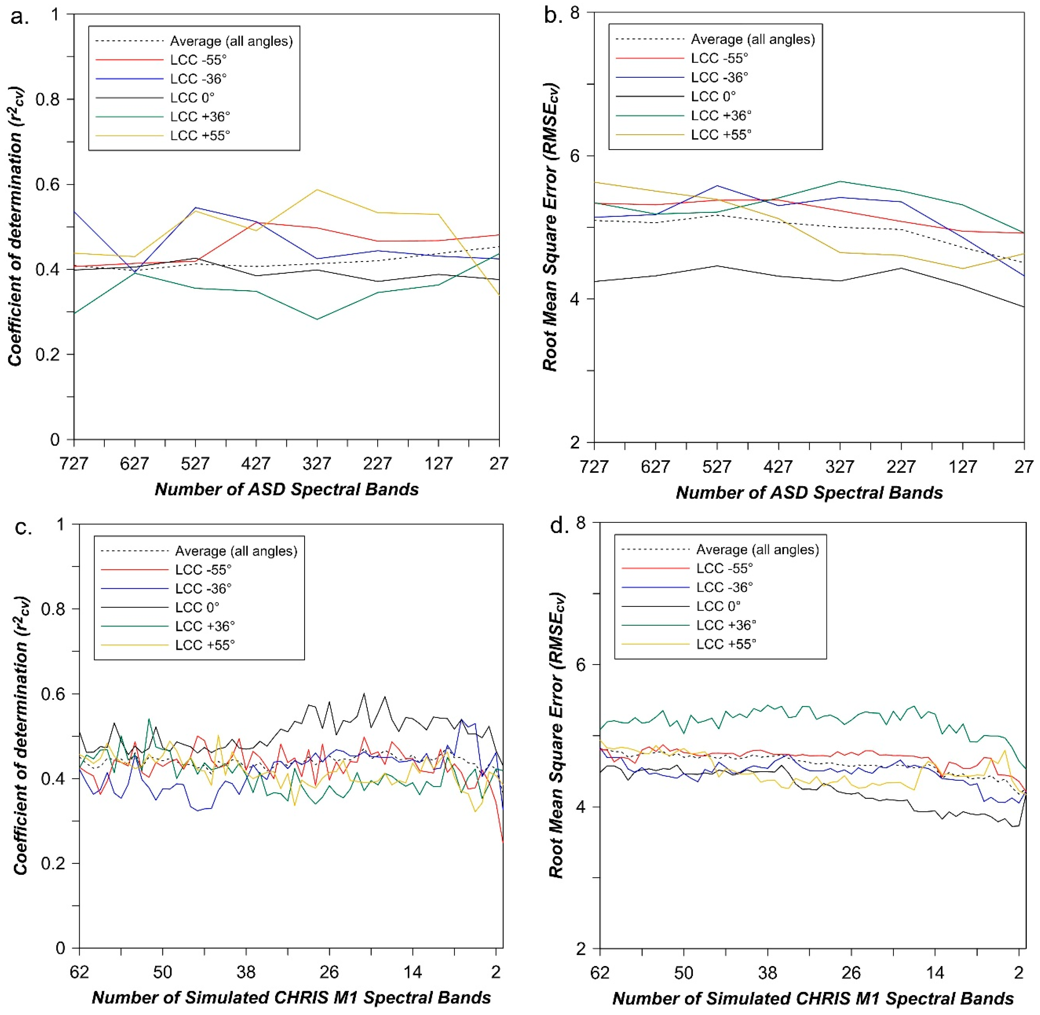
4.2.1. Multi-Band Vegetation Index Models

In general, many of the VIs performed similarly, suggesting that the wavelength regions used in a VI are more important than the VI formulation itself [91]. The two-band combinations that produced the highest r²_cv values for each VI were noticeably clustered in the visible around 350 nm and 550–600 nm, in the red-edge from 700 nm to 750 nm, and in the NIR from 950 nm to 1075 nm, with noticeable gaps of low r²_cv between these regions. These regions are as expected and similar to those found in Arctic field-based studies (e.g., [29,31]). Another important result is that r²_cv for the plot scale was almost always stronger than for the subplot scale. For the simple ratio (SR, discussed in more detail below), the differences in r²_cv shown in

Table 3. Two-band VIs ranked. Overall ranking of the top three VIs based on mean r²_cv and incorporates tests from all variables (e.g., LCC, PAI, and CCC), angles, scales, and spectral modes.

			ASD (Full Spectrum)		Simulated CHRIS M1
			Subplot	Plot	Subplot	Plot
VI	Rank	Mean r2cv	r2cv	r2cv	r2cv	r2cv
SR	1	0.51	0.48	0.58	0.45	0.53
NDVI	2	0.50	0.47	0.57	0.44	0.53
IPVI	3	0.50	0.46	0.57	0.44	0.53

were significant (p ≤ 0.05). Arctic vegetation canopies are highly variable at the 1 m² scale. This was also true for the narrowband VI regressions and GPR models and it concurs with Laidler et al. [49], showing that measurements should be averaged over larger homogeneous areas when retrieving Arctic biophysical and biochemical variables. Hereafter, only plot level (90 m × 90 m) results are presented.

Table 3 shows the top three results (r²_cv) of the ~2700 regression tests for the 11 multi-band VIs for the two spectral datasets (ASD full spectrum/simulated CHRIS M1 bands) and scales (subplot/plot) averaged over all sites, vegetation variables, and view angles (see [91] for a full list of indices and results). The evaluation of the VIs was based on the mean goodness-of fit statistics (r²) of the modeling results for all three vegetation variables combined (see [91]).

Given that most of the VIs performed quite similarly, SR was selected for further analysis since it is the simplest formulation, it was least affected by view angle geometry and it produced comparable results for LCC, PAI, and CCC. PAI model performance was best overall while LCC was the worst (

Table 4. SR model performance for plot scale data averaged over all sites and VZAs. RMSE_cv units: LCC (µg/cm²); PAI (unitless); CCC (g/m²). NRMSE_cv = RMSE_cv/range of measured data. The top angle-based results are highlighted and bolded.

		ASD (Full Spectrum)			Simulated CHRIS M1
Variable	Angle	r2cv	RMSEcv	NRMSEcv	r2cv	RMSEcv	NRMSEcv
LCC	All	0.54	3.29	0.11	0.47	3.45	0.11
PAI	All	0.64	0.17	0.15	0.58	0.19	0.17
CCC	All	0.56	0.08	0.11	0.53	0.08	0.12
LCC	+55°	0.57	3.24	0.11	0.46	3.43	0.11
LCC	+36°	0.56	3.31	0.11	0.44	3.39	0.11
LCC	0°	0.56	3.17	0.10	0.53	3.24	0.10
LCC	−36°	0.43	3.44	0.11	0.43	3.72	0.12
LCC	−55°	0.57	3.33	0.11	0.47	3.51	0.11
PAI	+55°	0.63	0.17	0.15	0.60	0.18	0.16
PAI	+36°	0.57	0.18	0.16	0.49	0.19	0.17
PAI	0°	0.69	0.16	0.14	0.60	0.18	0.17
PAI	−36°	0.69	0.18	0.15	0.63	0.19	0.16
PAI	−55°	0.62	0.17	0.15	0.58	0.19	0.17
CCC	+55°	0.60	0.08	0.11	0.51	0.08	0.12
CCC	+36°	0.59	0.08	0.11	0.50	0.09	0.12
CCC	0°	0.50	0.08	0.10	0.56	0.08	0.11
CCC	−36°	0.56	0.08	0.12	0.49	0.09	0.13
CCC	−55°	0.56	0.08	0.12	0.58	0.09	0.12
All	+55°	0.60	−	0.12	0.52	−	0.13
All	+36°	0.57	−	0.13	0.47	−	0.13
All	0°	0.58	−	0.12	0.57	−	0.12
All	−36°	0.56	−	0.13	0.52	−	0.14
All	−55°	0.58	−	0.13	0.54	−	0.14

). CCC model performance was in between PAI and LCC since it is a mathematical combination of both variables.

The narrower bands of the ASD data produced slightly better model fit and accuracy than the resampled CHRIS M1 data. The VZA that produced the best overall model fit for all three vegetation variables was +55° (mean r²_cv = 0.60) for the full ASD dataset; however, mean r²_cv values over all vegetation variables for each angle were comparable (within ±0.04). Modelled results were inclusive of all SZAs and SAAs for their respective forward and backscatter measurements; averaging of results dampened sun-sensor induced variations seen at the individual sites. Like the VI ranking (Table 3) the evaluation of the VZAs was based on the mean goodness-of fit statistics (r²) of the modeling results for all three vegetation variables combined [91].

Banks Island data produced better models (e.g., LCC: r²_cv = 0.78, RMSE_cv = 3.45; PAI: r²_cv = 0.94, RMSE_cv = 0.09; CCC r²_cv = 0.96, RMSE_cv = 0.03) than the other sites (e.g., Richardson Mountains 2013, LCC: r²_cv = 0.52, RMSE_cv = 3.88; PAI: r²_cv = 0.69, RMSE_cv = 0.12; CCC r²_cv = 0.50, RMSE_cv = 0.07). The strong results for Banks Island may be due to the large spatial variation in PAI values, where plots ranged from almost bare to completely covered with vegetation. Near zero values in the biochemical-biophysical variables help to ground the regression line and produce greater linearity. It is also possible that canopy height) played a role in the prediction strength. It was minimal in the high Arctic as compared to the greater vertical canopy complexity/height of the lower latitude sites, which can obscure some canopy elements. Figure 6 shows the best model predictions for each vegetation variable. The site and VZA are given; all best models were with ASD full spectrum data at the plot scale.

4.2.2. Predefined Narrowband VI models

The best overall narrowband VI was the Revised Optimized Soil Adjusted Vegetation Index (ROSAVI) [91,143]:

$$\begin{array}{c}ROSAVI=1.16\times \left(R_{750\mathrm{nm}}-R_{705\mathrm{nm}}\right)/\left(R_{750\mathrm{nm}}+R_{705\mathrm{nm}}+0.16\right)\end{array}$$

(1)

where R represents the reflectance at the indicated wavelength. ROSAVI produced an average r²_cv = 0.36 at the subplot scale and r²_cv = 0.54 at the plot scale for both the full ASD and simulated CHRIS M1 datasets. In total, ~20,000 (84 VIs × view angle × variable × spectral dataset × spatial scale) tests were performed (see [91] for a full list of indices and results). There were no significant differences between the top 20 (at least) narrowband VIs. The Blue Green Index (BGI) [144] produced almost identical results to ROSAVI. Other high performing VIs were also based on the Soil Adjusted Vegetation Index (SAVI) [145] and included OSAVI [146], TSAVI [147], and RMCARI [143], which is not surprising given the sparse nature and abundant non-green components of Arctic tundra vegetation. Even though the 10 nm bandwidth CHRIS bands often did not match the central wavelength of a given VI perfectly (e.g., 705/750 ROSAVI vs. 703/748 nm for CHRIS), both ASD and simulated CHRIS data produced almost identical model equations and performance for most VIs. This indicates that, contrary to the results for the SR analysis, bandwidth differences of 1–10 nm or a slight shift in central wavelength of the CHRIS bands from the specified VI wavelengths do not affect the vegetation models.

All narrowband VI models showed similar moderate strength at the plot scale, thus the choice of ROSAVI for further analysis (below) was somewhat arbitrary but representative of the other VIs.

Table 5. ROSAVI model performance for plot scale data averaged over all sites and VZAs. RMSE_cv units: LCC (µg/cm²); PAI (unitless); CCC (g/m²). NRMSE_cv = RMSE_cv/range of measured data. The top angle-based results are highlighted and bolded.

		ASD (Full Spectrum)			Simulated CHRIS M1
Variable	Angle	r2cv	RMSEcv	NRMSEcv	r2cv	RMSEcv	NRMSEcv
LCC	All	0.52	4.33	0.14	0.52	4.33	0.14
PAI	All	0.54	0.23	0.20	0.53	0.23	0.20
CCC	All	0.55	0.10	0.14	0.55	0.10	0.14
LCC	+55°	0.50	4.47	0.14	0.50	4.46	0.14
LCC	+36°	0.44	4.38	0.14	0.44	4.39	0.14
LCC	0°	0.57	3.97	0.12	0.58	3.98	0.12
LCC	−36°	0.51	4.51	0.14	0.52	4.52	0.14
LCC	−55°	0.57	4.39	0.14	0.57	4.38	0.14
PAI	+55°	0.53	0.21	0.19	0.53	0.21	0.19
PAI	+36°	0.56	0.23	0.20	0.56	0.23	0.20
PAI	0°	0.50	0.24	0.21	0.49	0.24	0.22
PAI	−36°	0.58	0.26	0.22	0.55	0.26	0.21
PAI	−55°	0.55	0.22	0.19	0.53	0.22	0.19
CCC	+55°	0.55	0.10	0.13	0.55	0.10	0.13
CCC	+36°	0.56	0.10	0.14	0.57	0.10	0.14
CCC	0°	0.51	0.10	0.13	0.50	0.10	0.13
CCC	−36°	0.56	0.12	0.16	0.57	0.12	0.16
CCC	−55°	0.58	0.09	0.13	0.58	0.10	0.13
All	+55°	0.52	−	0.15	0.53	−	0.15
All	+36°	0.52	−	0.16	0.52	−	0.16
All	0°	0.53	−	0.16	0.53	−	0.16
All	−36°	0.55	−	0.18	0.55	−	0.17
All	−55°	0.57	−	0.15	0.56	−	0.16

shows that model fit and prediction errors were generally slightly poorer than for SR (Table 4). However, simulated CHRIS M1 model performance was much closer to that for ASD full spectrum data, whereas it was markedly poorer for SR models. Model performance did not vary as much as for SR models across vegetation variables and VZAs for both spectral datasets. Contrary to the SR models, the VZA that produced the best overall model fit for all three vegetation variables was −55° (r²_cv = 0.57) for the full ASD dataset; r²_cv values were again comparable, being within ±0.05 for all VZAs. However, similar to the SR analysis, Banks Island (2012) data produced the strongest models (e.g., for −55°: LCC, r²_cv = 0.75, RMSE_cv = 5.61; PAI, r²_cv = 0.90, RMSE_cv = 0.10; CCC, r²_cv = 0.94, RMSE_cv = 0.04), compared to the poorest models, which were for Richardson Mountains (2013) data, with an average r²_cv = 0.38.

4.3. Non-Parametric Gaussian Process Regression Models

GPR models (

Table 6. GPR model performance for plot scale data averaged over all sites and VZAs. RMSE_cv units: LCC (µg/cm²); PAI (unitless); CCC (g/m²). NRMSE_cv = RMSE_cv/range of measured data. The top angle-based results are highlighted and bolded.

		ASD (Full Spectrum)			Simulated CHRIS M1
Variable	Angle	r2cv	RMSEcv	NRMSEcv	r2cv	RMSEcv	NRMSEcv
LCC	All	0.58	4.38	0.14	0.60	3.99	0.13
PAI	All	0.51	0.25	0.22	0.63	0.23	0.20
CCC	All	0.59	0.11	0.15	0.65	0.10	0.14
LCC	+55°	0.61	4.40	0.14	0.58	4.17	0.13
LCC	+36°	0.55	4.81	0.15	0.56	4.39	0.14
LCC	0°	0.53	3.95	0.12	0.66	3.61	0.11
LCC	−36°	0.61	4.04	0.13	0.57	3.79	0.12
LCC	−55°	0.59	4.81	0.15	0.62	4.12	0.13
PAI	+55°	0.44	0.25	0.22	0.54	0.22	0.19
PAI	+36°	0.48	0.25	0.21	0.65	0.22	0.19
PAI	0°	0.52	0.24	0.22	0.58	0.23	0.21
PAI	−36°	0.51	0.26	0.23	0.64	0.23	0.20
PAI	−55°	0.60	0.24	0.21	0.73	0.24	0.21
CCC	+55°	0.60	0.11	0.16	0.61	0.11	0.15
CCC	+36°	0.57	0.11	0.15	0.67	0.10	0.14
CCC	0°	0.54	0.10	0.14	0.59	0.10	0.13
CCC	−36°	0.61	0.11	0.15	0.69	0.10	0.14
CCC	−55°	0.62	0.11	0.16	0.70	0.11	0.16
All	+55°	0.55	−	0.17	0.58	−	0.16
All	+36°	0.53	−	0.17	0.62	−	0.16
All	0°	0.53	−	0.16	0.61	−	0.15
All	−36°	0.58	−	0.17	0.63	−	0.15
All	−55°	0.60	−	0.17	0.68	−	0.17

) generally performed better than VI-based regressions. In GPR iterative processing, as the least contributing bands were sequentially removed, r²_cv varied more for off-nadir view angles (Figure 7, LCC models given for illustrative purposes), and there was a slight increase in r²_cv as the number of variables was reduced (Figure 7a,c). Associated with this, RMSE tended to decrease as variables were removed (Figure 7b,d).

These trends were also manifested in the simulated CHRIS M1 data models (mean r²_cv = 0.62), which were stronger than models using all ASD narrow spectral bands (mean r²_cv = 0.56), and this result concurs with Verrelst et al. [24]. For LCC (Figure 7c), model performance was stable until approximately 10 bands were left, whereas for PAI and CCC, results were stable until there were as few as four bands left. For all vegetation variables; however, using only one or two bands produced the worst overall results, indicating that optimal models would require 5–10 bands for optimal performance.

With respect to VZA, −55° again produced the best overall results (mean r²_cv = 0.68 for the simulated CHRIS M1 data), while +55° produced the poorest models (mean r²_cv = 0.58). Among the study sites, Banks Island data again produced the best models (e.g., for −55°: LCC, r²_cv = 0.70, RMSE_cv = 5.14; PAI, r²_cv = 0.96, RMSE_cv = 0.10; CCC, r²_cv = 0.92, RMSE_cv = 0.05).

Finally, as for the iterative band optimization using SR, the GPR process ranked the bands by their frequency as the top band in the cross-validated regressions. The most important bands were consistently in the 450–500 nm (adjacent to peak green reflectance ~550 nm) and ~650–750 nm (chlorophyll absorption and red-edge) ranges for all three vegetation variables. This was expected, given the covariation of leaf and canopy chlorophyll with plant area index.

4.4. Physical Modelling: PROSAIL Simulations and Inversion

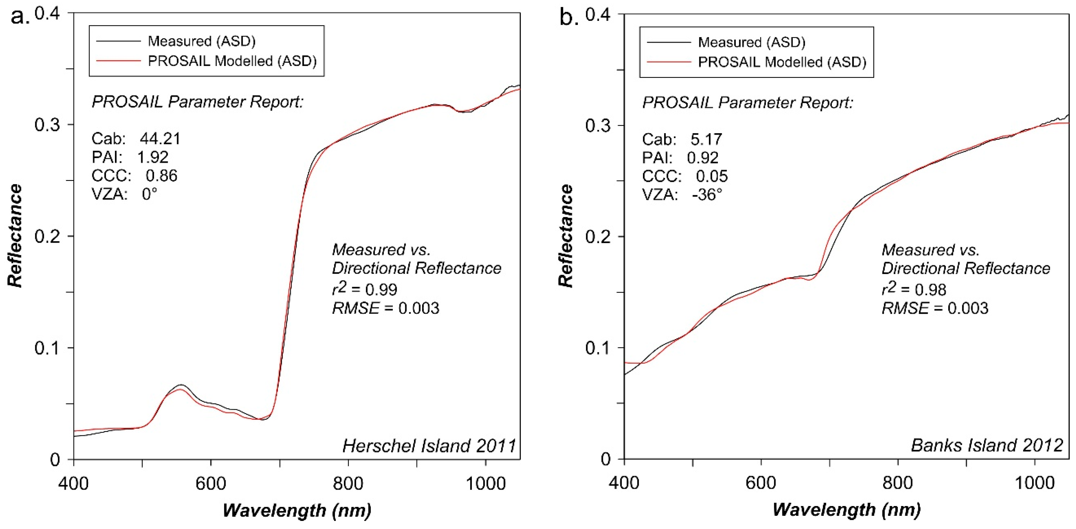
4.4.1. Spectral Curve Fitting Validation

The LM inversion curve fitting algorithm was capable of reproducing TOC directional-reflectance for all value ranges of LCC, PAI, and CCC, (i.e., low to high values) and at all VZAs (mean r² = 0.99; mean RMSE = 0.4% ± 0.2%). These results may be partially due to spatial averaging of subplots into plot scale measurements; more noise was observed in subplot spectra and this propagated through the inversion procedure. Figure 8a,b shows two example spectra representing the range from dense to sparse vegetation cover. Inverted modelled parameters are shown for each curve. Local minima were not encountered in the modelling process, supporting the approach of providing the best possible estimates for initial model values [121]. Optimum curve fitting was achieved with more than 100 iterations (5000 iterations were used for all final modelling); poor results were achieved with 1–50 iterations. The use of too many fixed variables also caused the LM inversion to behave erratically; using value ranges may be of greater importance than fixing parameters for such iterative optimization.

The greatest observed error between the measured and modelled spectra occurred in the lower wavelength regions (e.g., <~500 nm) and generally occurred as an over-prediction (i.e., modelled PROSAIL TOC reflectance values were greater than measured TOC reflectance values). Figure 8c,d shows the differences between the modelled and measured reflectance values for various sites and VZAs (modelled values were subtracted from measured values to better show over and under prediction of PROSAIL). Reflectance at these wavelengths was either not well measured, related to the inherent noise associated with the spectroradiometer, or not well modelled by the PROSAIL RTM. Similarly, large error was observed in the longer wavelength regions (>~900 nm); however, in contrast to the shorter wavelength regions, these regions commonly produced under-predictions of TOC reflectance. Error patterns (both over and under predictions) were observed across the peak green reflectance (~550 nm), chlorophyll absorption (~680 nm), and red-edge regions (~700–750 nm) for all sites and VZAs. Although it could be stated that the degree of error for most spectral regions was well within ±0.02 (or 2%), it is possible that these three regions are also not well modelled by PROSAIL in Arctic environments due to the complexity of the canopy (i.e., number of species, pigment pools) and the degree of spatial variation to canopy structure across all sites (i.e., gap fractions, soil contributions).

The LUT-based inversions produced spectral fits that were poorer than the LM approach, often possessing reflectance errors that were in excess of 0.02 (2%). In general, the greatest errors occurred in similar wavelength regions as the LM inversion for all variables, VZAs, and field sites. Because the mean of multiple best solutions approach was used for the LUT inversions (i.e., larger spectral ranges are considered valid in the inversion process), it was expected that spectral fits would not necessarily be as good as the LM curve fitting algorithm as valid spectral matches (and associated parameters) were allowed to range from 0 to 20%.

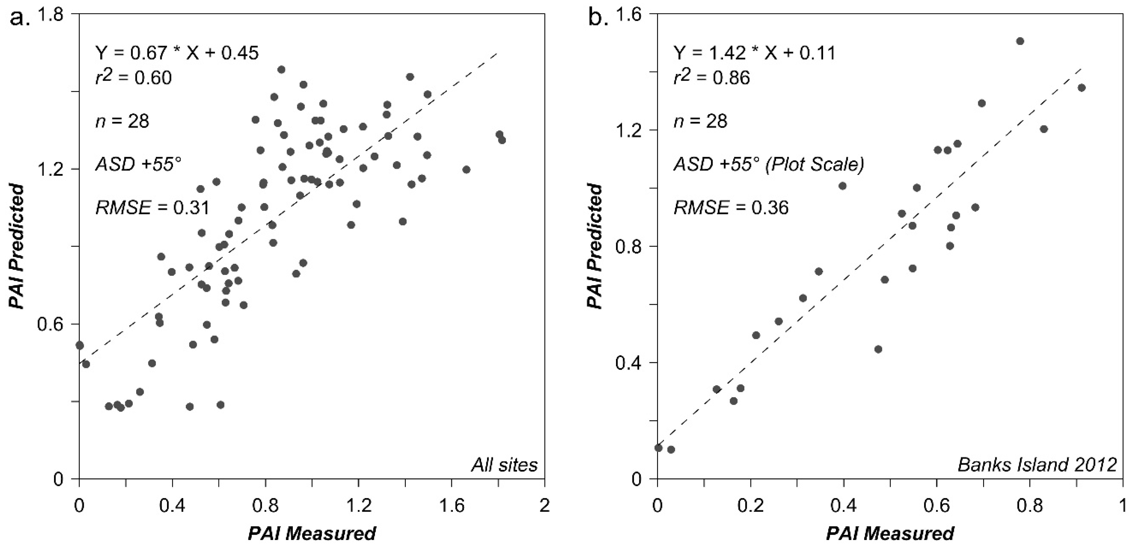
4.4.2. Vegetation Modelling: PROSAIL LM Inversion

The performance of the PROSAIL LM inversion to estimate LCC, PAI, and CCC (

Table 7. PROSAIL LM model performance for plot scale data averaged over all sites and VZAs. RMSE units: LCC (µg/cm²); PAI (unitless); CCC (g/m²). NRMSE = RMSE/range of measured data. The top angle-based results are highlighted and bolded.

		ASD (Full Spectrum)			Simulated CHRIS M1
Variable	Angle	r2	RMSE	NRMSE	r2	RMSE	NRMSE
LCC	All	0.35	8.31	0.28	0.28	7.74	0.27
PAI	All	0.28	0.44	0.42	0.27	0.41	0.38
CCC	All	0.36	0.18	0.25	0.29	0.16	0.23
LCC	+55°	0.33	8.88	0.29	0.20	8.44	0.28
LCC	+36°	0.25	9.18	0.31	0.24	8.14	0.29
LCC	0°	0.46	7.23	0.25	0.34	6.97	0.23
LCC	−36°	0.32	9.44	0.32	0.32	7.96	0.27
LCC	−55°	0.35	7.10	0.26	0.31	7.39	0.28
PAI	+55°	0.35	0.40	0.37	0.30	0.38	0.36
PAI	+36°	0.22	0.48	0.46	0.25	0.44	0.41
PAI	0°	0.36	0.43	0.41	0.26	0.41	0.40
PAI	−36°	0.20	0.49	0.45	0.29	0.40	0.37
PAI	−55°	0.27	0.41	0.38	0.23	0.40	0.37
CCC	+55°	0.48	0.18	0.25	0.22	0.17	0.24
CCC	+36°	0.30	0.19	0.26	0.30	0.17	0.24
CCC	0°	0.49	0.15	0.21	0.34	0.16	0.21
CCC	−36°	0.22	0.19	0.26	0.27	0.16	0.23
CCC	−55°	0.28	0.18	0.26	0.31	0.16	0.23
All	+55°	0.39	−	0.30	0.24	−	0.30
All	+36°	0.26	−	0.34	0.26	−	0.31
All	0°	0.44	−	0.29	0.31	−	0.28
All	−36°	0.25	−	0.35	0.29	−	0.29
All	−55°	0.30	−	0.30	0.28	−	0.29

) was not as good as the empirical modelling (ASD spectra: mean r² = 0.33; simulated CHRIS M1 spectra: mean r² = 0.28). CCC and LCC were better modelled than PAI; this contrasts with the empirical models and with other studies using PROSAIL that have reported better models for LAI than LCC (e.g., [19,20]).

Of the VZAs, nadir (0°) produced the best overall results (r² = 0.44), followed by +55° (r² = 0.39) for the full spectrum ASD dataset. Similar to the empirical analyses, Banks Island data produced the strongest models (LCC: r² = 0.76, RMSE = 9.94; PAI: r² = 0.64, RMSE = 0.64; CCC: r² = 0.79, RMSE = 0.12, for ASD spectra averaged over all VZAs). The Banks Island model fit for LCC was as strong as for the empirical models but the RMSE was much higher using the LM inversion.

4.4.3. Vegetation Modelling: PROSAIL LUT Inversion

The LUT inversion produced superior results (

Table 8. PROSAIL LUT-based model performance for plot scale data averaged over all sites and VZAs. RMSE units: LCC (µg/cm²); PAI (unitless); CCC (g/m²). NRMSE = RMSE/range of measured data. Cost functions are displayed using the following superscripts: a RMSE, b. Neyman chi-square, c. Geman and McClure, d. LSE, and e. Bhattacharyya divergence. Optimal cost functions were selected based on a combination of r², RMSE, and NRMSE. The top angle-based results are highlighted and bolded.

		ASD (Full Spectrum)			Simulated CHRIS M1
Variable	Angle	r2	RMSE	NRMSE	r2	RMSE	NRMSE
LCC	All	0.44 a	6.67	0.15	0.46 a	6.37	0.14
PAI	All	0.55 b	0.53	0.29	0.52 b	0.47	0.26
CCC	All	0.46 b	0.18	0.23	0.43 b	0.18	0.23
LCC	+55°	0.45 a	6.89	0.16	0.47 a	6.34	0.14
LCC	+36°	0.38 d	8.37	0.19	0.39 a	7.08	0.16
LCC	0°	0.55 d	6.88	0.16	0.54 a	5.90	0.13
LCC	−36°	0.45 d	7.93	0.18	0.44 d	7.92	0.18
LCC	−55°	0.49 a	6.05	0.14	0.50 a	6.02	0.14
PAI	+55°	0.60 b	0.31	0.17	0.53 b	0.28	0.15
PAI	+36°	0.56 b	0.44	0.24	0.51 b	0.38	0.21
PAI	0°	0.53 b	0.45	0.25	0.48 b	0.38	0.21
PAI	−36°	0.54 b	0.62	0.34	0.52 b	0.56	0.31
PAI	−55°	0.53 a	0.75	0.41	0.53 e	0.75	0.41
CCC	+55°	0.53 b	0.12	0.15	0.48 a	0.14	0.18
CCC	+36°	0.45 c	0.14	0.18	0.41 b	0.15	0.19
CCC	0°	0.49 b	0.14	0.18	0.46 b	0.13	0.17
CCC	−36°	0.42 a	0.18	0.23	0.40 e	0.18	0.23
CCC	−55°	0.45 a	0.29	0.37	0.44 a	0.28	0.36
All	+55°	0.50 b	−	0.17	0.48 a	−	0.17
All	+36°	0.46 c	−	0.21	0.42 b	−	0.19
All	0°	0.50 b	−	0.20	0.48 b	−	0.18
All	−36°	0.44 a	−	0.22	0.42 a	−	0.22
All	−55°	0.50 a	−	0.31	0.50 a	−	0.30

) to the LM inversion and to the LHS LUT for estimating LCC, PAI, and CCC (ASD spectra: mean r² = 0.48; simulated CHRIS M1 spectra: mean r² = 0.46). LHS field tests were subsequently discarded from the analysis. When used in conjunction with regularization approaches, such as the addition of noise and the use of multiple best solutions, results were comparable to the field-based ROSAVI retrievals (e.g., r² difference of 0.06; NRMSE difference of 0.08). The best ASD inversions were achieved with the addition of ~9% Gaussian noise and the mean of the top ~10% best spectral matches, whereas the CHRIS M1 benefited from ~12% Gaussian noise and the mean of the top ~12% best spectral matches. When averaged across variables, VZAs, and sensors configurations, the best performing cost function was RMSE (NRMSE=0.21); however, best results were achieved with the Neyman chi-square for both PAI and CCC when averaged across VZAs and sensor configurations (NRMSE=0.28 and NRMSE=0.23, respectively).

Of the VZAs, nadir (0°) and the extreme view zenith angles (±55°) produced the best overall correlation results (mean r² = 0.50), followed by ±36° (mean r² = 0.45) for the full spectrum ASD dataset; however, the best predictions accuracies were achieved at +55 for both sensor configurations (NRMSE = 0.17) and the worst at −55° (NRMSE = 0.31). Like all previous analyses, Banks Island produced the strongest models (LCC: r² = 0.57, RMSE = 8.59; PAI: r² = 0.86, RMSE = 0.59; CCC: r² = 0.74, RMSE = 0.12, for ASD spectra averaged over all VZAs) although a positive bias was observed in all models for all vegetation variables. Figure 9 shows the best LUT inversion results for PAI using data for the entire bioclimatic dataset (a) and for the Banks Island site (b) for the +55° VZA. PAI produced the best overall model fits followed by CCC though LCC had the lowest overall error (e.g., NRMSE = 0.14 for the CHRIS M1 dataset).

4.4.4. Comparison of VI Retrievals Using Simulated Multi-Angle Spectra

Results of the PROSAIL/VI sensitivity analysis (

Table 9. SR and ROSAVI model performance for plot scale data averaged over all sites and VZAs using the LHS PROSAIL simulated CHRIS M1 dataset. RMSE_cv units: LCC (µg/cm²); PAI (unitless); CCC (g/m²). NRMSE_cv = RMSE_cv/range of measured data. The top angle-based results are highlighted and bolded.

		SR (Simulated CHRIS M1)			ROSAVI (Simulated CHRIS M1)
Variable	Angle	r2	RMSE	NRMSE	r2	RMSE	NRMSE
LCC	All	0.48	11.67	0.18	0.52	11.29	0.17
PAI	All	0.72	0.39	0.13	0.61	0.46	0.15
CCC	All	0.77	0.15	0.09	0.64	0.18	0.11
LCC	+55°	0.57	10.71	0.16	0.59	10.45	0.16
LCC	+36°	0.54	11.02	0.17	0.56	10.75	0.16
LCC	0°	0.52	11.28	0.17	0.55	10.93	0.17
LCC	−36°	0.45	12.12	0.18	0.49	11.64	0.18
LCC	−55°	0.34	13.19	0.20	0.39	12.70	0.19
PAI	+55°	0.76	0.37	0.12	0.66	0.43	0.14
PAI	+36°	0.74	0.38	0.13	0.66	0.43	0.14
PAI	0°	0.72	0.39	0.13	0.65	0.44	0.15
PAI	−36°	0.71	0.40	0.13	0.62	0.46	0.15
PAI	−55°	0.67	0.42	0.14	0.45	0.55	0.18
CCC	+55°	0.82	0.13	0.08	0.68	0.18	0.11
CCC	+36°	0.80	0.14	0.09	0.67	0.18	0.11
CCC	0°	0.78	0.14	0.09	0.67	0.18	0.11
CCC	−36°	0.75	0.15	0.10	0.65	0.18	0.11
CCC	−55°	0.69	0.17	0.11	0.55	0.21	0.55
All	+55°	0.71	−	0.12	0.64	−	0.14
All	+36°	0.69	−	0.13	0.63	−	0.14
All	0°	0.67	−	0.13	0.62	−	0.14
All	−36°	0.63	−	0.14	0.59	−	0.15
All	−55°	0.57	−	0.15	0.46	−	0.17

) showed the following. (1) Forward scatter spectra produced the best overall model fits and had the lowest overall error (e.g., SR VI r² = 0.71, NRMSE=0.12 for +55° VZA) relative to backscatter receivals (e.g., r² = 0.57, NRMSE = 0.15 for −55° VZA). The LUT-based inversions for both the ASD and M1 datasets produced similar trends for retrieval accuracy as they relate to VZA (i.e., increasing from forward to backscatter); however, model fits did not follow the same pattern as the theoretical VI retrievals (i.e., decreasing from forward to backscatter) but instead showed no clear trend. The SR VI empirical retrievals showed that the best overall model was achieved at +55° VZA for the ASD dataset, although marginal, the ROSAVI and GPR showed the opposite. (2) CCC was the most accurately retrieved vegetation variable followed by PAI and LCC respectively for both the SR and ROSAVI models with simulated data. Modelling with field data produced similar results (r²) for both ROSAVI (both datasets) and GPR (for the M1 dataset), but accuracies (NRMSE) were not necessarily the best for CCC. In contrast, all retrievals (empirical and physical) using the full bioclimatic field dataset showed that PAI had the highest overall errors. (3) The best overall retrievals using the simulated LHS dataset were achieved with the SR VI (r² = 0.66, NRMSE = 0.13) as compared to the ROSAVI (r² = 0.59, NRMSE = 0.15); however, ROSAVI produced slightly better results for LCC. The empirical modelling using the field dataset produced similar results, where the multi-band SR was overall better than using predefined narrow bands in the ROSAVI formulation. Finally, the VI field-based retrievals produced similar modelling results to the simulated retrievals when using the mean of all vegetation variables and VZAs (e.g., difference of r² = 0.08 and NRMSE = 0.01 for SR; and a difference of r ²= 0.05 and NRMSE = 0.02 for ROSAVI), thus demonstrating that the PROSAIL model provides a reasonably accurate spectral representation of Arctic tundra directional reflectance (given the variable parameter space used) at the plot scale for the visited field sites.

5. Discussion

A field-based, multi-angle, multi-method spectroscopic analysis of Arctic vegetation was conducted in the Western Canadian Arctic. New contributions include: (1) characterization of leaf and canopy vegetation biochemistry at four different sites across a bioclimatic gradient from north central Yukon Territory to the northern end of Banks Island in the Beaufort Sea; (2) multi-angle reflectance analysis across the same environments; (3) comparison of parametric and non-parametric empirical modelling approaches for estimation of LCC, PAI and CCC; and (4) comparison of empirical models with the physically based PROSAIL model for estimation of the same variables. Models were evaluated at two spatial scales (plot and subplot), using full visible-NIR spectra and simulated CHRIS M1 spectral bands.

5.1. Comparison of Field Measurements across a Bioclimatic Gradient

There are very few studies that have quantified the pigments of Arctic vegetation at the field scale. Tieszen and Johnson [148] measured pigment structures for four different species in northern Alaska; chlorophyll values of 32 to 77 μg/cm² were reported. Early spectrophotometry studies such as this are invaluable; however, the extinction coefficients used in the spectrophotometry analysis were from Arnon [149] and have been deemed incorrect [102]. In our research, field-measured chlorophyll concentrations of the dominant species sampled were between 10.5 μg/cm² to 57.2 μg/cm² (37.5 μg/cm² average). (Table 1). This average value is similar to the 38.0 μg/cm² reported in Tiezsen and Johnson [148]; however, the range of values reported were quite different despite measuring similar species (e.g., cotton grass). The values reported here were derived using updated and accepted extinction coefficients [102]. Leaf chlorophyll exhibited a gradient from higher LCC at lower latitudes (e.g., ~40.7 μg/cm²) to lower LCC at higher latitudes (e.g., ~32.0 μg/cm²), and this gradient was also evident in CCC values. Such latitudinal Arctic LCC and CCC values have not been previously reported. The destructive lab/field-based chlorophyll measurements showed no statistical difference (p < 0.05) to plot-scale handheld chlorophyll measurements when converted using a consensus equation [95], thus indicating the potential for the generalized use of such handheld chlorophyll meters in the Arctic.

Although not the primary focus of the modelling retrievals in this research, measurement of carotenoid and EWT values was important for parameterization of the PROSAIL model. Carotenoid concentrations of the dominant species ranged from 3.3 μg/cm² to 23.0 μg/cm² (average = 14.6 μg/cm²), while EWT values ranged from 0.01 g/cm² to 0.04 g/cm² (average = 0.03 g/cm²). Subsequent vegetation-based biochemical research conducted in the Arctic should focus on comprehensive characterization of pigment and non-pigment vegetation biochemistry across species, seasons, and representative environments. Not only would such a dataset serve as baseline/reference data for retrieval studies but would allow for further refinement of RTMs that are increasingly incorporating additional leaf/canopy parameters into their code (e.g., PROSPECT-D) [39].

5.2. Multi-Angle Spectroscopic Analysis across a Bioclimatic Gradient

Multi-angle spectroscopic analysis showed that top-of-canopy reflectance possessed angular dependencies, with peak variability centered on the chlorophyll absorption region (~680 nm), and low variability evident at peak green reflectance (~550 nm) and regions related to leaf and canopy structure (≥~700 nm). The low reflectance variability observed at all sites around ~550 nm may be due to consistent quantities of leaf/canopy carotenoid content found within and across Arctic vegetation species/assemblages. Whereas the higher variability of reflectance found at ~680 nm may be attributable to a high degree of leaf/canopy chlorophyll differences found between species and sites. Since chlorophyll degrades rapidly in comparison to carotenoids when plants undergo stress or senescence [140,141,142], the large differences in variability between these two spectral regions (i.e., chlorophyll:carotenoid ratios) may point towards a means of better understanding seasonal changes across a variety of environmental conditions, species, and functional types that are found in the Arctic [5,150].

Negative VZAs generally produced the greatest reflectance as expected for backscatter spectra where shadows are minimized by the relatively small angular difference between the sensor and illumination source (i.e., the sun) (Figure 5a,b). Nadir reflectance was generally lowest across the full spectral range, providing evidence that tundra does not act as a specular or diffuse reflector (more related to volume scattering) and that, like other ecosystems, nadir measurements are highly affected by canopy gaps and shadows [5]. Increased gap fraction can decrease the quality and magnitude of the reflectance signal [5,137,138]. Spectra measured across all field sites and VZAs were not typical of dense green vegetation, particularly for the northern sites, but were similar to those of other Arctic studies (e.g., [29,31,43]) where visible soil/substrates and non-photosynthetic vegetation components caused a general progressive increase in reflectance across the visible, red-edge, and NIR regions. Red-edge reflectance in the southern sites exhibited a greater slope compared to the northern sites for the same reasons; indeed, LCC and PAI (and associated canopy gap fractions) decreased with increasing latitude. These results concur with previous studies; however, the comprehensive analysis presented here for multiple field sites on a latitudinal gradient, different spectral data sets and different spatial scales (plot and subplot) provided a strong basis for the empirical and physical modelling at both the field and satellite imaging scales [71].

5.3. Empirical Modelling: Comparison of Parametric and Non-Parametric Retrieval Methods

Parametric and non-parametric regression analyses showed that prediction of LCC, PAI and CCC was most consistent and least sensitive to angular effects when using the simple ratio (SR) with optimally selected spectral bands (Table 4). Of the 11 two-band VIs tested, NDVI produced similar results to SR (Table 3). It has also been investigated in the Arctic using a similar band selection procedure with moderate to good success but using nadir data only (e.g., [29]). Optimal wavelengths found in this study concurred with Liu et al. [29] and were, as expected, in the red absorption region and the red-edge/NIR region influenced by vegetation structure. However, the large range of optimal wavelengths (~615–700 nm and ~710–880 nm, respectively) is directly related to reflectance anisotropy, which has not previously been reported for Arctic tundra ecosystems with respect to vegetation parameter retrievals [69].

Non-parametric GPR produced the overall best r²_cv (Table 6), and this was with the simulated CHRIS M1 dataset, but it had slightly poorer mean predictive capability than SR. The use of the full spectrum data led to poorer GPR performance as also reported by Verrelst et al. [24]. Multi-collinearity and noisy bands should be reduced/removed using band selection based on expert knowledge or quantitative techniques (e.g., principal component analysis). In this study, the simulated CHRIS M1 dataset of 62, 10 nm bands within the range of 411 nm to 997 nm accomplished both reduction of multi-collinearity and removal of noisy bands at both ends of the ASD spectral range, resulting in enhanced results over full spectrum narrowband data. This concurs with other studies for crops (e.g., [24,151]) but this is the first time it has been demonstrated in Arctic vegetation.

Many of the pre-defined narrowband VIs performed almost as well as the optimized SR and GPR. Of the 65 VIs, four SAVI-based VIs were among the top ten (ROSAVI, OSAVI, TSAVI, and RMCARI) [91]. ROSAVI performed the best overall irrespective of VZA and vegetation variable (Table 5); its wavelengths (705 nm and 750 nm) are within the range of the optimal spectral bands selected for SR. Soil-based VIs (e.g., SAVI variants) have been extensively tested in agriculture contexts but have been applied less in vegetation modelling/retrieval testing in natural ecosystems (e.g., [143]). Furthermore, SAVI-based VIs have been tested less in Arctic environments compared to other traditional VIs such as NDVI (e.g., [29,31]). The results here show that they are well suited to the sparse canopies and overall additive influence of soils and other non-green vegetation components of Arctic tundra.

The best estimates of LCC, PAI, and CCC were achieved at the plot scale for all empirical modelling techniques. Subplot (1 m²) measurements were more spatially variable; reduction of such variability is important when scaling up to moderate resolution satellite scales. The best estimates for all techniques were also achieved in the high Arctic, concurring with Liu et al. [29] who also produced good models in the high Arctic using narrowband VIs. This suggests that low-statured two-dimensional canopies produce better models because vegetation elements (i.e., leaves) are not obscured as in more vertically complex canopies.

With respect to VZA, optimal r²_cv values were generally achieved at −55° with empirical approaches, although r²_cv did not vary much with VZA. Relative model prediction error was lowest for 0° but also did not vary much with VZA. Other studies have found that off-nadir observations are more useful since less background is visible within the field of view [152] and backscatter has been found to be better than forward scatter [153,154,155]. However, this does not always hold true. For example, Stagakis et al. [5] found retrieval of chlorophyll, carotenoids, and LAI to be best at +55° within a Mediterranean ecosystem due to reduced soil background effects; i.e., for that ecosystem soil background influences were deemed to be more important than shadow effects. This reasoning may also hold in the Arctic due to the low stature and density of the canopy (potentially less overall influence of shadow due to vertical canopy structure); canopy gaps in tundra vegetation (especially at high latitudes) will inevitably lead to increased soil exposure. This is supported by Verrelst et al. [68], who reported significant reflectance and VI anisotropy in pine forest and meadow and concluded that the proportions of photosynthetic, non-photosynthetic and background compounds are stronger drivers than shadow. However, it is likely that shadows caused by tussocks, shrubs, hummocks at forward scatter view angles play a more significant role in directional reflectance than backgrounds and soils where there is 100% canopy cover due to their size relative to the individual canopy elements (i.e., leaves/needles and stems). The grade of the slope in which plots were situated/sampled may have contributed to the variability of the shadowing; however, steep slopes where not sampled. Combined results of the empirical analyses showed that canopy structure (i.e., PAI) is best retrieved at −55°; however, results were not substantially different for the other VZAs. This suggests that in low statured tundra canopies structural attributes (e.g., PAI and gap fractions) can be observed and extracted similarly from both forward and backscatter VZAs. Finally, since spectral measurements made at each VZA integrated a range of SZA and SAA values, future research (i.e., biophysical and biochemical retrievals using empirical modelling approaches) should examine the effect that fine-scale solar angular variability observed in both forward and backscatter domains has on model performance. Expressing sun-sensor geometries as phase angle may prove useful (e.g., [156]).

5.4. Physical Modelling: Assessment of PROSAIL and Comparison of Inversion Techniques

The PROSAIL model when inverted with the LUT approach achieved results that were comparable to the empirical models (Table 8). The LM-based approach, however, did not achieve the same overall performance (Table 7). PAI was typically better modelled and estimated than LCC and CCC with the LUT approach, and like the field-based SR results, CCC retrievals were comparable to LCC when averaged across field sites and VZAs. It was expected that CCC results would be similar or better than LCC and PAI since it is derived from a combination of LCC and PAI and both are known to conjointly control canopy reflectance across the visible-near infrared spectrum [5,20,21,24,157]. It should be noted that CCC is correlated with plant density and community/assemblage as it uses both LCC and PAI in its formulation and is not depicting only PAI values. Where vegetation is denser (in a continuous or a discontinuous canopy) there will be greater quantities of chlorophyll aggregated across the canopy, given the same plant phenological conditions and assemblages/species between ground plots. We observed the same plants/communities existing at various densities—in these circumstances CCC is more a function of density (or PAI). Where different plant assemblages with different levels of chlorophyll exist in similar densities, CCC is more related to leaf chlorophyll, as this will be different across the canopy between the ground plots. PAI models were the poorest with the LM approach but reflectance error was only about ±0.02 on the red-edge and the left wing of the NIR, which are regions known to be sensitive to Arctic leaf and canopy structure [29,31]. The optimal LUT-based results differ from those studies that have shown difficulties in estimating LCC with PROSAIL in heterogeneous plant assemblages given prediction errors were within 15% [20,158,159], but align with studies that show LAI is easier to predict than LCC [20,160].

The overall poor results of the LM inversions may be explained by the inability of the one-dimension PROSAIL turbid medium model to accurately describe the directional radiation field of a complex heterogeneous canopy. However, the results of the LUT retrievals, the similarity of the simulated PROSAIL SR retrievals (Table 9) to the field-based SR retrievals (Table 4), and the good performance of all inversion models at the field site with the greatest PAI variability/separability (i.e., Banks Island) indicate that inversion errors may instead be due to the sampled variable’s parameter space (i.e., the separation in PAI values) and model ill-posedness.

Improvement in variable retrieval using either inversion approach may require consideration of canopy heterogeneity effects such as clumping, varying leaf and canopy structures (e.g., PAI), and pigment variability as it relates to species and/or functional groups present (e.g., [39,161]). Darvishzadeh et al. [20] showed that low-level, heterogeneous grassland canopies can be simulated with PROSAIL when stratification of plant heterogeneity (based on the number of species present) is integrated. A similar approach using the stratification of Arctic tundra vegetation based on species numbers would be a difficult undertaking due to the natural mixture of species at the subplot scale (1 m²) and would not be practical to implement within an ecosystem monitoring program; however, it may be possible that measuring biochemical and biophysical plant traits from distinct functional groups/species assemblages may be a way of stratifying the sample measurement space for maximal parameter separation (see [162,163]). Nevertheless, the use of PROSAIL may be of value to monitoring monotypic shrub patches as their abundance increases across the Arctic [74,79] and as high spatial and spectral resolution sensors become more available.

Our explanations for better results at higher latitudes/lower biomass sites are as follows. (a) It is important to sample the full range of values (both spectral and biophysical/biochemical) at each site as this will allow for greater differentiation in the model predictions (i.e., separability in predicted values and/or classes). The Banks Island site contained greater PAI contrast between plots compared to other sites. (b) The physical model ill-posedness is related to the variability of the sampled parameters; i.e., where there is less spatial variability between spectral and biophysical/biochemical values, less differentiation will be seen between plots, thus leading to higher confusion in the inversion. It may be that the PROSAIL algorithms cannot distinguish the fine spectral differences between vegetation communities/parameters (e.g., where differences of LCC=34 µg/cm² vs. 35 µg/cm² occur) at a more uniform site than at a spatially heterogeneous site, as can be seen in Figure 5. We concluded that the one-dimensional PROSAIL turbid medium can be successfully applied in tundra environments where there is significant spatial variability between plots (when fine spatial scale variability has been accounted for/removed through proper field sampling approaches) and where broader classes of biophysical and biochemical variables are used that have a greater degree of separation. Indeed, when we grouped the LCC datasets into 5 µg/cm² classes and inverted the mean spectra from these classes, results were good for both LM and LUT inversion techniques (e.g., r²=0.89 to 0.92, respectively), though this should be interpreted with caution as these classes may not correspond to distinct vegetation types or assemblages that are geographically locatable. The implementation of a three-dimensional modelling approach (e.g., DART, [164,165]) may be more appropriate for high spatial resolution sensor applications in Arctic environments (e.g., [58]) but may have their own limitations (e.g., proper parameterization and inversion). PROSAIL is commonly applied and understood by many researchers so, in selecting an appropriate approach for this first such modelling study in Arctic environments, this study provides a baseline for which other biochemical and biophysical retrieval studies can be improved. From here, we expect others to try to improve on the results we found with refinements or different physical modelling approaches.

The poor results obtained by the LM inversion can typically be attributed to model ill-posedness; it is a well-known problem that multiple parameter combinations will lead to the same spectral reflectance [19,40]. LM was therefore considered extremely susceptible to ill-posedness as only one set of parameters was produced from each inversion. Attempts were made to account for ill-posedness and local minima by employing commonly used regularization strategies, including (a) setting the minimum and maximum values for each parameter based on field measurements and accepted ranges based on the literature, (b) setting algorithm start values based on average leaf/canopy conditions, and (c) fixing algorithm variables with known fixed parameters (e.g., VZAs).

The LUT approach was able to produce superior results to the LM approach when steps were taken to account for ill-posedness and should, therefore, be considered as the optimal approach for predicting biochemical and biochemical variables in tundra environments. The inversion of PROSAIL model against plot-scale ASD full spectrum and CHRIS M1 simulated hyperspectral data and a field-based validation dataset led to the following conclusions about cost functions, regularization options, and parameterization data. (a) The systematic evaluation of cost functions for inversion of biophysical and biochemical parameters in Arctic environments has not previously been conducted but have been evaluated in agricultural landscapes [59]. Divergence measures (i.e., RMSE and Neyman chi-square) were the best performing, with RMSE having the best results across all vegetation variables and Neyman chi-square performing best with PAI and CCC regardless of VZA. These results differ from that of Rivera et al. [59], who showed that LCC was best retrieved with LAE, while LAI was best retrieved with LSE. It is recommended that future inversion studies examine the use data normalization when implementing LUT inversion approaches. (b) The optimal inversion cost functions benefited from the addition of ~9–12% Gaussian noise and the use of the mean of the top 10–12% of spectral matches. These results are similar to those achieved by Rivera et al. [59] who showed that the using 6% of multiple solutions and the addition of <20% noise yielded best results for retrieval of LCC and LAI in agricultural areas. The addition of noise and multiple best solutions provides further insight into why stratification is important to achieving optimal results in tundra environments. The degree of spectral separation between similar vegetation values (e.g., PAI values of 0.10 vs. 0.15) may be too small of a difference to overcome with current inversion techniques. (c) The use of prior information was shown to benefit the LUT-based inversion approach. For example, we compared the following: (i) the inversion of multiple view angles (i.e., all five angles) from the field spectroscopy data using one parametrized PROSAIL LUT that used one view angle (e.g., nadir); and (ii) the inversion of one field spectroscopy view angle (e.g., nadir) to multiple PROSAIL LUTs that were parameterized with all view zenith angles. In both cases, results were very similar to those achieved using the correctly parameterized angular parameters (VZA). This result further highlights the problem of ill-posedness that can be encountered within the realm of physical modelling. It also highlights that angular information based on view angle may not be as important as correctly parameterizing the other leaf/canopy variables in the PROSAIL model. The results of this simple test highlight the need to provide as many correctly parameterized values as possible in the inversion approach regardless of approach taken and regularization strategies used. It is recommended that inversion studies be accompanied by high-quality calibration/validation field data; however, where these are not available, the values provided here can serve as a baseline for tundra vegetation biochemical and biophysical parameters.

Spectral subsets using coarser spectral sampling (i.e., the M1 simulated CHRIS/PROBA, bandwidths of ~10 nm) produced slightly less accurate predictions for all modelling approaches as compared to the full spectrum narrow bands (<2 nm). This outcome appears to support the notion that narrower bands provide better exploitation of subtle absorption and reflectance features of Arctic vegetation. However, the results of the predefined narrowband vegetation analysis of this study suggest that a bandwidth difference of ~2 to ~10 nm has no effect (as reported for the ROSAVI results). An explanation for better performance with the ASD dataset compared to the simulated CHRIS/PROBA M1 data may be that band center positions for the CHRIS sensor are not in the optimal locations for detecting Arctic tundra vegetation biochemical and biophysical properties. It is possible that full spectrum data that include short-wavelength infrared regions may provide additional benefits for retrieving and mapping biochemical and biophysical variables in Arctic environments and should be explored in future research (e.g., AVRISI-NG, EnMAP, PRISMA), especially with the physical modelling approach. In addition, the removal of spectral bands that are not well simulated by PROSAIL should be explored as this may increase inversion retrieval performance (e.g., [21]).

6. Conclusions

Arctic tundra vegetation properties of leaf and canopy chlorophyll content and plant area index were modelled using multi-angle field spectroscopy. Empirical parametric and non-parametric regression techniques were compared to the physically-based PROSAIL model. In empirical analysis, optimization of band selection for two-band vegetation indices was compared to pre-defined narrowband indices. Analyses were conducted using data acquired at four sites from the low to high Arctic, at two spatial scales (field and satellite remote sensing, and for two spectral datasets (full spectrum and simulated CHRIS M1 bands). Overall conclusions are as follows. (1) The simple ratio (SR) and revised optimized soil adjusted vegetation index (ROSAVI) were the optimal two-band and predefined narrowband multi-angle VIs, respectively. (2) The GPR algorithm produced favorable results when used in combination with a spectrally reduced dataset (i.e., CHRIS M1). (3) The optimal multi-angle spectral regions for variable retrievals were largely 450–550 nm and 650–750 nm. The −55° view angle produced better empirical retrievals results. However, the overall conclusion drawn from the compiled empirical and physical modelling results, when examined across the field sites, was that a multi-angle approach (view angles within ±55°) provides comparable/viable characterizations of vegetated surfaces and are therefore equally suitable for biochemical and biophysical variable retrievals in the Arctic. (4) The PROSAIL model, when implemented with a field-based spectral data and inverted using a LUT approach (accompanied with appropriate cost functions and regularization approaches), was determined to be suitable for the prediction of LCC, PAI, and CCC in Arctic environments when vegetation variables are separated into distinct numerical classes (i.e., grouped ranges of values ordered in sequence).

References

1. Kokaly, R.F.; Asner, G.P.; Ollinger, S.V.; Martin, M.E.; Wessman, C.A. Characterizing canopy biochemistry from imaging spectroscopy and its application to ecosystem studies. Remote Sens. Environ. 2009, 113, S78–S91. [Google Scholar] [CrossRef]
2. Ustin, S.L.; Gitelson, A.A.; Jacquemoud, S.; Schaepman, M.E.; Asner, G.P.; Gamon, J.A.; Zarco-Tejada, P.J. Retrieval of foliar information about plant pigment systems from high resolution spectroscopy. Remote Sens. Environ. 2009, 113, S67–S77. [Google Scholar] [CrossRef] [Green Version]
3. Schaepman, M.E.; Ustin, S.L.; Plaza, A.J.; Painter, T.H.; Verrelst, J.; Liang, S. Earth system science related imaging spectroscopy: An assessment. Remote Sens. Environ. 2009, 113, S123–S137. [Google Scholar] [CrossRef]
4. Borzuchowski, J.; Schulz, K. Retrieval of leaf area index (LAI) and soil water content (WC) using hyperspectral remote sensing under controlled glass house conditions for spring barley and sugar beet. Remote Sens. 2010, 2, 1702–1721. [Google Scholar] [CrossRef] [Green Version]
5. Stagakis, S.; Markos, N.; Sykioti, O.; Kyparissis, A. Monitoring canopy biophysical and biochemical parameters in ecosystem scale using satellite hyperspectral imagery: An application on a Phlomis fruticosa Mediterranean ecosystem using multi-angular CHRIS/PROBA observations. Remote Sens. Environ. 2010, 114, 977–994. [Google Scholar] [CrossRef]
6. Sykioti, O.; Paronis, D.; Stagakis, S.; Kyparissis, A. Band depth analysis of CHRIS/PROBA data for the study of a Mediterranean natural ecosystem. Correlations with leaf optical properties and ecophysiological parameters. Remote Sens. Environ. 2011, 115, 752–766. [Google Scholar] [CrossRef]
7. Chapin, F.S.; Sturm, M.; Serreze, M.C.; McFadden, J.P.; Key, J.R.; Lloyd, A.H.; McGuire, A.D.; Rupp, T.S.; Lynch, A.H.; Schimel, J.P.; et al. Role of land-surface changes in Arctic summer warming. Science 2005, 310, 657–660. [Google Scholar] [CrossRef] [PubMed]
8. Jia, G.J.; Epstein, H.E.; Walker, D.A. Vegetation greening in the Canadian Arctic related to decadal warming. J. Environ. Monit. 2009, 11, 2231–2238. [Google Scholar] [CrossRef]
9. Stow, D.A.; Hope, A.; McGuire, D.; Verbyla, D.; Gamon, J.; Huemmrich, F.; Houston, S.; Racine, C.; Sturm, M.; Tape, K.; et al. Remote sensing of vegetation and land-cover change in Arctic Tundra Ecosystems. Remote Sens. Environ. 2004, 89, 281–308. [Google Scholar] [CrossRef] [Green Version]
10. Gamon, J.A.; Huemmrich, K.F.; Stone, R.S.; Tweedie, C.E. Spatial and temporal variation in primary productivity (NDVI) of coastal Alaskan tundra: Decreased vegetation growth following earlier snowmelt. Remote Sens. Environ. 2013, 129, 144–153. [Google Scholar] [CrossRef] [Green Version]
11. Walker, D.A.; Raynolds, M.K.; Daniëls, F.J.; Einarsson, E.; Elvebakk, A.; Gould, W.A.; Katenin, A.E.; Kholod, S.S.; Markon, C.J.; Melnikov, E.S.; et al. The Circumpolar Arctic Vegetation Map (CAVM). J. Veg. Sci. 2005, 16, 267–282. [Google Scholar] [CrossRef]
12. Raynolds, M.K.; Walker, D.A.; Balser, A.; Bay, C.; Campbell, M.; Cherosov, M.M.; Daniëls, F.J.A.; Eidesen, P.B.; Ermokhina, K.A.; Frost, G.V.; et al. A raster version of the Circumpolar Arctic Vegetation Map (CAVM). Remote Sens. Environ. 2019, 232, 111297. [Google Scholar] [CrossRef]
13. Chapman, J.W.; Thompson, D.R.; Helmlinger, M.C.; Bue, B.D.; Green, R.O.; Eastwood, M.L.; Geier, S.; Olson-Duvall, W.; Lundeen, S.R. Spectral and radiometric calibration of the Next Generation Airborne Visible Infrared Spectrometer (AVIRIS-NG). Remote Sens. 2019, 11, 2129. [Google Scholar] [CrossRef] [Green Version]
14. Galeazzi, C.; Sacchetti, A.; Cisbani, A.; Babini, G. The PRISMA Program. In Proceedings of the IGARSS 2008—2008 IEEE International Geoscience and Remote Sensing Symposium, Boston, MA, USA, 7–11 July 2008; pp. IV—105–IV—108. [Google Scholar]
15. Kaufmann, H.; Segl, K.; Chabrillat, S.; Hofer, S.; Stuffier, T.; Mueller, A.; Richter, R.; Schreier, G.; Haydn, R.; Bach, H. EnMAP—A hyperspectral sensor for environmental mapping and analysis. In Proceedings of the 2006 IEEE International Symposium on Geoscience and Remote Sensing, Denver, CO, USA, 31 July–4 August 2006; pp. 1617–1619. [Google Scholar]
16. Blackburn, G.A. Quantifying chlorophylls and carotenoids at leaf and canopy scales: An evaluation of some hyperspectral approaches. Remote Sens. Environ. 1998, 66, 273–285. [Google Scholar] [CrossRef]
17. Blackburn, G.A. Spectral indices for estimating photosynthetic pigment concentrations: A test using senescent tree leaves. Int. J. Remote Sens. 1998, 19, 657–675. [Google Scholar] [CrossRef]
18. Blackburn, G.A. Hyperspectral remote sensing of plant pigments. J. Exp. Bot. 2007, 58, 855–867. [Google Scholar] [CrossRef] [Green Version]
19. Darvishzadeh, R.; Skidmore, A.; Schlerf, M.; Atzberger, C.; Corsi, F.; Cho, M. LAI and chlorophyll estimated for a heterogeneous grassland using hyperspectral measurements. ISPRS J. Photogramm. Remote Sens. 2008, 63, 409–426. [Google Scholar] [CrossRef]
20. Darvishzadeh, R.; Skidmore, A.; Schlerf, M.; Atzberger, C. Inversion of a radiative transfer model for estimating vegetation LAI and chlorophyll in a heterogeneous grassland. Remote Sens. Environ. 2008, 112, 2592–2604. [Google Scholar] [CrossRef]
21. Darvishzadeh, R.; Atzberger, C.; Skidmore, A.; Schlerf, M. Mapping grassland leaf area index with airborne hyperspectral imagery: A comparison study of statistical approaches and inversion of radiative transfer models. ISPRS J. Photogramm. Remote Sens. 2011, 66, 894–906. [Google Scholar] [CrossRef]
22. Dorigo, W.A.; Zurita-Milla, R.; de Wit, A.J.W.; Brazile, J.; Singh, R.; Schaepman, M.E. A review on reflective remote sensing and data assimilation techniques for enhanced agroecosystem modeling. Int. J. Appl. Earth Obs. Geoinf. 2007, 9, 165–193. [Google Scholar] [CrossRef]
23. Barnsley, M.J.; Settle, J.J.; Cutter, M.A.; Lobb, D.R.; Teston, F. The PROBA/CHRIS mission: A low-cost small sat for hyperspectral multiangle observations of the earth surface and atmosphere. IEEE Trans. Geosci. Remote Sens. 2004, 42, 1512–1520. [Google Scholar] [CrossRef]
24. Verrelst, J.; Rivera, J.; Gitelson, A.; Delegido, J.; Moreno, J.; Camps-Valls, G. Spectral band selection for vegetation properties retrieval using Gaussian processes regression. Int. J. Appl. Earth. Obs. Geoinf. 2016, 52, 554–567. [Google Scholar] [CrossRef]
25. Curran, P.J. Remote sensing of foliar chemistry. Remote Sens. Environ. 1989, 30, 271–278. [Google Scholar] [CrossRef]
26. Grossman, Y.L.; Ustin, S.L.; Jacquemoud, S.; Sanderson, E.W.; Schmuck, G.; Verdebout, J. Critique of stepwise multiple linear regression for the extraction of leaf biochemistry information from leaf reflectance data. Remote Sens. Environ. 1996, 56, 182–193. [Google Scholar] [CrossRef]
27. Clevers, J.; Kooistra, L.; van den Brande, M. Using Sentinel-2 Data for retrieving LAI and Leaf and Canopy Chlorophyll content of a potato crop. Remote Sens. 2017, 9, 405. [Google Scholar] [CrossRef] [Green Version]
28. Croft, H.; Chen, J.M.; Zhang, Y. The applicability of empirical vegetation indices for determining leaf chlorophyll content over different leaf and canopy structures. Ecol. Complex. 2014, 17, 119–130. [Google Scholar] [CrossRef]
29. Liu, N.; Budkewitsch, P.; Treitz, P. Examining spectral reflectance features related to Arctic percent vegetation cover: Implications for hyperspectral remote sensing of Arctic tundra. Remote Sens. Environ. 2017, 192, 58–72. [Google Scholar] [CrossRef]
30. Verrelst, J.; Camps-Valls, G.; Muñoz-Marí, J.; Rivera, J.; Veroustraete, F.; Clevers, J.; Moreno, J. Optical remote sensing and the retrieval of terrestrial vegetation bio-geophysical properties: A review. ISPRS J. Photogramm. Remote Sens. 2015, 108, 273–290. [Google Scholar] [CrossRef]
31. Buchhorn, M.; Walker, D.A.; Heim, B.; Raynolds, M.K.; Epstein, H.E.; Schwieder, M. Ground-Based hyperspectral characterization of Alaska tundra vegetation along environmental gradients. Remote Sens. 2013, 5, 3971–4005. [Google Scholar] [CrossRef] [Green Version]
32. Verrelst, J.; Rivera, J.; Veroustraete, F.; Munoz-Mari, J.; Clevers, J.; Camps-Valls, G.; Moreno, J. Experimental Sentinel-2 LAI estimation using parametric, non-parametric and physical retrieval methods: A comparison. ISPRS J. Photogramm. Remote Sens. 2015, 108, 260–272. [Google Scholar] [CrossRef]
33. Jacquemoud, S.; Verhoef, W.; Baret, F.; Bacour, C.; Zarco-Tejada, P.J.; Asner, G.P.; François, C.; Ustin, S.L. PROSPECT+SAIL models: A review of use for vegetation characterization. Remote Sens. Environ. 2009, 113, S56–S66. [Google Scholar] [CrossRef]
34. Feret, J.B.; François, C.; Asner, G.P.; Gitelson, A.A.; Martin, R.E.; Bidel, L.P.R.; Ustin, S.L.; le Maire, G.; Jacquemoud, S. PROSPECT-4 and 5: Advances in the leaf optical properties model separating photosynthetic pigments. Remote Sens. Environ. 2008, 112, 3030–3043. [Google Scholar] [CrossRef]
35. Jacquemoud, S.; Baret, F. PROSPECT: A model of leaf optical properties spectra. Remote Sens. Environ. 1990, 34, 75–91. [Google Scholar] [CrossRef]
36. Verhoef, W. Light scattering by leaf layers with application to canopy reflectance modelling: The SAIL model. Remote Sens. Environ. 1984, 16, 125–141. [Google Scholar] [CrossRef] [Green Version]
37. Verhoef, W. Earth observation modeling based on layer scattering matrices. Remote Sens. Environ. 1985, 17, 165–178. [Google Scholar] [CrossRef] [Green Version]
38. Berger, K.; Atzberger, C.; Danner, M.; D’Urso, G.; Mauser, W.; Vuolo, F.; Hank, T. Evaluation of the PROSAIL model capabilities for future hyperspectral model environments: A review study. Remote Sens. 2018, 10, 85. [Google Scholar] [CrossRef] [Green Version]
39. Feret, J.B.; Gitelson, A.A.; Noble, S.D.; Jacquemoud, S. PROSPECT-D: Towards modeling leaf optical properties through a complete lifecycle. Remote Sens. Environ. 2017, 193, 204–215. [Google Scholar] [CrossRef] [Green Version]
40. Combal, B.; Baret, F.; Weiss, M. Improving canopy variables estimation from remote sensing data by exploiting ancillary information. Case study on sugar beet canopies. Agronomie 2002, 22, 205–215. [Google Scholar] [CrossRef]
41. Combal, B.; Baret, F.; Weiss, M.; Trubuil, A.; Mace, D.; Pragnere, A.; Myneni, R.; Knyazikhin, Y.; Wang, L. Retrieval of canopy biophysical variables from bidirectional reflectance: Using prior information to solve the ill-posed inverse problem. Remote Sens. Environ. 2003, 84, 1–15. [Google Scholar] [CrossRef]
42. Baret, F.; Buis, S. Estimating canopy characteristics from remote sensing observations. Review of methods and associated problems. In Advances in Land Remote Sensing: System, Modeling, Inversion and Application; Liang, S., Ed.; Springer: Berlin/Heidelberg, Germany, 2008; pp. 171–200. [Google Scholar]
43. Bratsch, S.N.; Epstein, H.E.; Buchhorn, M.; Walker, D.A. Differentiating among four Arctic tundra plant communities at Ivotuk, Alaska using field spectroscopy. Remote Sens. 2016, 8, 51. [Google Scholar] [CrossRef] [Green Version]
44. Davidson, S.; Santos, M.; Sloan, V.; Watts, J.; Phoenix, G.; Oechel, W.; Zona, D. Mapping Arctic Tundra vegetation communities using field spectroscopy and multispectral satellite data in North Alaska, USA. Remote Sens. 2016, 8, 978. [Google Scholar] [CrossRef] [Green Version]
45. Hope, A.S.; Kimball, J.S.; Stow, D.A. The relationship between tussock tundra spectral reflectance properties and biomass and vegetation composition. Int. J. Remote Sens. 1993, 14, 1861–1874. [Google Scholar] [CrossRef]
46. Huemmrich, K.F.; Gamon, J.A.; Tweedie, C.E.; Campbell, P.K.; Landis, D.R.; Middleton, E.M. Arctic tundra vegetation functional types based on photosynthetic physiology and optical properties. IEEE J. Sel. Top. Appl. Earth Obs. Remote Sens. 2013, 6, 265–275. [Google Scholar] [CrossRef] [Green Version]
47. Kushida, K.; Kim, Y.; Tsuyuzaki, S.; Fukuda, M. Spectral vegetation indices for estimating shrub cover, green phytomass and leaf turnover in a sedge-shrub tundra. Int. J. Remote Sens. 2009, 30, 1651–1658. [Google Scholar] [CrossRef]
48. Kushida, K.; Hobara, S.; Tsuyuzaki, S.; Kim, Y.; Watanabe, M.; Setiawan, Y.; Harada, K.; Shaver, G.R.; Fukuda, M. Spectral indices for remote sensing of phytomass, deciduous shrubs, and productivity in Alaskan Arctic tundra. Int. J. Remote Sens. 2015, 36, 4344–4362. [Google Scholar] [CrossRef]
49. Laidler, G.J.; Treitz, P.M.; Atkinson, D.M. Remote sensing of Arctic vegetation: Relations between the NDVI, Spatial Resolution and Vegetation Cover on Boothia Peninsula, Nunavut. Arctic 2008, 61, 1–13. [Google Scholar] [CrossRef] [Green Version]
50. Riedel, S.M.; Epstein, H.E.; Walker, D.A. Biotic controls over spectral reflectance of Arctic tundra vegetation. Int. J. Remote Sens. 2005, 26, 2391–2405. [Google Scholar] [CrossRef]
51. Riedel, S.M.; Epstein, H.E.; Walker, D.A.; Richardson, D.L.; Calef, M.P.; Edwards, E.; Moody, A. Spatial and temporal heterogeneity of vegetation properties among four tundra plant communities at Ivotuk, Alaska, USA. Arct. Antarct. Alp. Res. 2005, 37, 25–33. [Google Scholar] [CrossRef]
52. Ulrich, M.; Grosse, G.; Chabrillat, S.; Schirrmeister, L. Spectral characterization of periglacial surfaces and geomorphological units in the Arctic Lena Delta using field spectrometry and remote sensing. Remote Sens. Environ. 2009, 113, 1220–1235. [Google Scholar] [CrossRef] [Green Version]
53. Ma, L.; Liu, Y.; Zhang, X.; Ye, Y.; Yin, G.; Johnson, B.A. Deep learning in remote sensing applications: A meta-analysis and review. ISPRS J. Photogramm. Remote Sens. 2019, 152, 166–177. [Google Scholar] [CrossRef]
54. Rasmussen, C.E.; Williams, C.K.I. Gaussian Processes for Machine Learning; The MIT Press: New York, NY, USA, 2006. [Google Scholar]
55. Verrelst, J.; Muñoz, J.; Alonso, L.; Delegido, J.; Rivera, J.P.; Camps-Valls, G.; Moreno, J. Machine learning regression algorithms for biophysical parameter retrieval: Opportunities for Sentinel-2 and -3. Remote Sens. Environ. 2012, 118, 127–139. [Google Scholar] [CrossRef]
56. Verrelst, J.; Alonso, L.; Rivera Caicedo, J.P.; Moreno, J.; Camps-Valls, G. Gaussian process retrieval of chlorophyll content from imaging spectroscopy data. IEEE J. Sel. Top. Appl. Earth Obs. Remote Sens. 2013, 6, 867–874. [Google Scholar] [CrossRef]
57. Wang, Z.; Townsend, P.A.; Schweiger, A.K.; Couture, J.J.; Singh, A.; Hobbie, S.E.; Cavender-Bares, J. Mapping foliar functional traits and their uncertainties across three years in a grassland experiment. Remote Sens. Environ. 2019, 221, 405–416. [Google Scholar] [CrossRef]
58. Juszak, I.; Iturrate-Garcia, M.; Gastellu-Etchegorry, J.P.; Schaepman, M.E.; Maximov, T.C.; Schaepman-Strub, G. Drivers of shortwave radiation fluxes in Arctic tundra across scales. Remote Sens. Environ. 2017, 193, 86–102. [Google Scholar] [CrossRef] [Green Version]
59. Rivera, J.P.; Verrelst, J.; Leonenko, G.; Moreno, J. Multiple cost functions and regularization options for improved retrieval of leaf chlorophyll content and LAI through inversion of the PROSAIL model. Remote Sens. 2013, 5, 3280–3304. [Google Scholar] [CrossRef] [Green Version]
60. Zarco-Tejada, P.J.; Rueda, C.A.; Ustin, S.L. Water content estimation in vegetation with MODIS reflectance data and model inversion methods. Remote Sens. Environ. 2003, 85, 109–124. [Google Scholar] [CrossRef]
61. Hilker, T.; Galvão, L.S.; Aragão, L.; de Moura, Y.M.; do Amaral, C.H.; Lyapustin, A.I.; Wu, J.; Albert, L.P.; Ferreira, M.J.; Anderson, L.O.; et al. Vegetation chlorophyll estimates in the Amazon from multi-angle MODIS observations and canopy reflectance model. Int. J. Appl. Earth. Obs. Geoinf. 2017, 58, 278–287. [Google Scholar] [CrossRef] [Green Version]
62. Casas, A.; Riaño, D.; Ustin, S.L.; Dennison, P.; Salas, J. Estimation of water-related biochemical and biophysical vegetation properties using multitemporal airborne hyperspectral data and its comparison to MODIS spectral response. Remote Sens. Environ. 2014, 148, 28–41. [Google Scholar] [CrossRef]
63. Hilker, T.; Gitelson, A.; Coops, N.C.; Hall, F.G.; Black, T.A. Tracking plant physiological properties from multi-angular tower-based remote sensing. Oecologia 2011, 165, 865–876. [Google Scholar] [CrossRef] [Green Version]
64. Schaepman, M.E. Spectrodirectional remote sensing: From pixels to processes. Int. J. Appl. Earth Obs. Geoinf. 2007, 9, 204–223. [Google Scholar] [CrossRef] [Green Version]
65. Chopping, M.; Moisen, G.G.; Su, L.; Laliberte, A.; Rango, A.; Martonchik, J.V.; Peters, D.P.C. Large area mapping of southwestern forest crown cover, canopy height, and biomass using the NASA Multiangle Imaging Spectro-Radiometer. Remote Sens. Environ. 2008, 112, 2051–2063. [Google Scholar] [CrossRef] [Green Version]
66. Diner, D.J.; Asner, G.P.; Davies, R.; Knyazikhin, Y.; Muller, J.; Nolin, A.W.; Pinty, B.; Schaaf, C.B.; Stroeve, J. New directions in earth observing: Scientific applications of multi-angle remote sensing. Bull. Am. Meteorol. Soc. 1999, 80, 2209–2228. [Google Scholar] [CrossRef] [Green Version]
67. Diner, D.J.; Braswell, B.H.; Davies, R.; Gobron, N.; Hu, J.; Jin, Y.; Kahn, R.A.; Knyazikhin, Y.; Loeb, N.; Muller, J.P.; et al. The value of multiangle measurements for retrieving structurally and radiatively consistent properties of clouds, aerosols, and surfaces. Remote Sens. Environ. 2005, 97, 495–518. [Google Scholar] [CrossRef]
68. Verrelst, J.; Schaepman, M.E.; Koetz, B.; Kneubühler, M. Angular sensitivity analysis of vegetation indices derived from CHRIS/PROBA data. Remote Sens. Environ. 2008, 112, 2341–2353. [Google Scholar] [CrossRef]
69. Vierling, L.A.; Deering, D.W.; Eck, T.F. Differences in Arctic tundra vegetation type and phenology as seen using bidirectional radiometry in the early growing season. Remote Sens. Environ. 1997, 60, 71–82. [Google Scholar] [CrossRef]
70. Buchhorn, M.; Raynolds, M.K.; Walker, D.A. Influence of BRDF on NDVI and biomass estimations of Alaska Arctic tundra. Environ. Res. Lett. 2016, 11, 125002. [Google Scholar] [CrossRef]
71. Kennedy, B.E.; King, D.J.; Duffe, J. Retrieval of Arctic Vegetation biophysical and biochemical properties from CHRIS/PROBA Multi-Angle Imaging Spectroscopy using empirical and PROSAIL physical modelling. Manuscript in preparation.
72. Ecological Stratification Working Group (ESWG). A National Ecological Framework for Canada; Report and National Map at 1:7500 000 Scale; Agriculture and Agri-Food Canada; Research Branch; Centre for Land and Biological Resources Research and Environment Canada; State of the Environment Directorate; Ecozone Analysis Branch: Ottawa, ON, Canada, 1995. [Google Scholar]
73. Bhatt, U.S.; Walker, D.A.; Raynolds, M.K.; Comiso, J.C.; Epstein, H.E.; Jia, G.; Gens, R.; Pinzon, J.E.; Tucker, C.J.; Tweedie, C.E.; et al. Circumpolar Arctic tundra vegetation change is linked to sea ice decline. Earth Interact. 2010, 14, 1–20. [Google Scholar] [CrossRef] [Green Version]
74. Fraser, R.H.; Lantz, T.C.; Olthof, I.; Kokelj, S.V.; Sims, R.A. Warming-Induced Shrub Expansion and Lichen Decline in the Western Canadian Arctic. Ecosystems 2014, 17, 1151–1168. [Google Scholar] [CrossRef]
75. Fraser, R.H.; Olthof, I.; Kokelj, S.V.; Lantz, T.C.; Lacelle, D.; Brooker, A.; Wolfe, S.; Schwarz, S. Detecting landscape changes in high latitude environments using Landsat trend analysis: 1. Visualization. Remote Sens. 2014, 6, 11533–11557. [Google Scholar] [CrossRef] [Green Version]
76. Myers-Smith, I.H.; Hik, D.S.; Kennedy, C.; Cooley, D.; Johnstone, J.F.; Kenney, A.J.; Krebs, C.J. Expansion of canopy-forming willows over the twentieth century on Herschel Island, Yukon Territory, Canada. Ambio 2011, 40, 610–623. [Google Scholar] [CrossRef]
77. Olthof, I.; Fraser, R.H. Detecting landscape changes in high latitude environments using Landsat trend analysis: 2. classification. Remote Sens. 2014, 6, 11558–11578. [Google Scholar] [CrossRef] [Green Version]
78. Pouliot, D.; Latifovic, R.; Olthof, I. Trends in vegetation NDVI from1 km AVHRR data over Canada for the period 1985–2006. Int. J. Remote Sens. 2009, 30, 149–168. [Google Scholar] [CrossRef]
79. Sturm, M.; Racine, C.; Tape, K. Increasing shrub abundance in the Arctic. Nature 2001, 411, 546–547. [Google Scholar] [CrossRef]
80. Walker, D.A.; Daniëls, F.J.A.; Alsos, I.; Bhatt, U.S.; Breen, A.L.; Buchhorn, M.; Bültmann, H.; Druckenmiller, L.A.; Edwards, M.E.; Ehrich, D.; et al. Circumpolar Arctic vegetation: A hierarchic review and roadmap toward an internationally consistent approach to survey, archive and classify tundra plot data. Environ. Res. Lett. 2016, 11, 55005. [Google Scholar] [CrossRef]
81. Myneni, R.B.; Keeling, C.D.; Tucker, C.J.; Asrar, A.; Nemani, R.R. Increased plant growth in the northern high latitudes from 1981 to 1991. Nature 1997, 386, 698–702. [Google Scholar] [CrossRef]
82. Burn, C.R.; Kokelj, S.V. The environment and permafrost of the Mackenzie Delta area. Permafr. Periglac. Process. 2009, 20, 83–105. [Google Scholar] [CrossRef]
83. Hinzman, L.D.; Bettez, N.D.; Bolton, W.R.; Chapin, F.S.; Dyurgerov, M.B.; Fastie, C.L.; Griffith, B.; Hollister, R.D.; Hope, A.; Huntington, H.P.; et al. Evidence and implications of recent climate change in northern Alaska and other Arctic regions. Clim. Chang. 2005, 72, 251–298. [Google Scholar] [CrossRef]
84. Serreze, M.C.; Walsh, J.E.; Chapin, F.S.; Osterkamp, T.; Dyurgerov, M.; Romanovsky, V.; Oechel, W.C.J.; Morison, W.C.; Zhang, T.; Barry, R.G. Observational evidence of recent change in the Northern high-latitude environment. Clim. Chang. 2000, 46, 159–207. [Google Scholar] [CrossRef]
85. Natural Resources Canada. Atlas of Canada National Scale Data 1:1,000,000. Ottawa, Ontario, Canada: Natural Resources Canada. 2014. Available online: http://open.canada.ca/data/en/dataset/e9931fc7-034c-52ad-91c5-6c64d4ba0065 (accessed on 1 October 2016).
86. Natural Resources Canada. Atlas of Canada, Northern Geodatabase. Ottawa, Ontario, Canada: Natural Resources Canada. 2012. Available online: http://open.canada.ca/data/en/dataset/7e388083-6b66-5e0e-a264-a3c0eb98a2f0 (accessed on 1 October 2016).
87. CAFF (Conservation of Arctic Flora and Fauna). Arctic Biodiversity Assessment: Status and Trends in Arctic Biodiversity; Conservation of Arctic Flora and Fauna: Akureyri, Iceland; Narayana Press: Odder, Denmark, 2013. [Google Scholar]
88. Daniëls, F.J.; Gillespie, L.J.; Poulin, M. Plants. In Arctic Biodiversity Assessment: Status and Trends in Arctic Biodiversity; Meltofte, H., Ed.; Conservation of Arctic Flora and Fauna: Akureyri, Iceland; Narayana Press: Odder, Denmark, 2013; pp. 310–353. [Google Scholar]
89. Elvebakk, A. Tundra diversity and ecological characteristics of Svalbard. In Ecosystems of the World; Wielgolaski, F., Ed.; Elsevier: Oxford, UK, 1997; Volume 3, pp. 347–359. [Google Scholar]
90. Walker, D.A.; Auerbach, N.A.; Bockheim, J.G.; Chapin, F.S., III; Eugster, W.; King, J.Y.; McFadden, J.P.; Michaelson, G.J.; Nelson, F.E.; Oechel, W.C.; et al. Energy and trace-gas fluxes across a soil pH boundary in the Arctic. Nature 1998, 394, 469–472. [Google Scholar] [CrossRef]
91. Kennedy, B.E. Multi-Angle Spectroscopic Remote Sensing of Arctic Vegetation Biochemical and Biophysical Properties. Ph.D. Thesis, Carleton University, Ottawa, ON, Canada, 2017. [Google Scholar]
92. Neumann, H.H.; Hartog, G.D.; Shaw, R.H. Leaf area measurements based on hemispheric photographs and leaf-litter collection in a deciduous forest during autumn leaf-fall. Agric. For. Meteorol. 1989, 45, 325–345. [Google Scholar] [CrossRef]
93. Mougin, E.; Demarez, V.; Diawara, M.; Hiernaux, P.; Soumaguel, N.; Berg, A. Estimation of LAI, fAPAR and fCover of Sahel rangelands (Gourma, Mali). Agric. For. Meteorol. 2014, 198, 155–167. [Google Scholar] [CrossRef]
94. Campbell, R.J.; Nobley, K.N.; Marini, R.P.; Pfeiffer, D.G. Growing conditions alter the relationship between SPAD-501 values and apple leaf chlorophyll. HortScience 1990, 25, 330–331. [Google Scholar] [CrossRef] [Green Version]
95. Cerovic, Z.; Masdoumier, G.; Ghozlen, N.; Latouche, G. A new optical leaf-clip meter for simultaneous non-destructive assessment of leaf chlorophyll and epidermal flavonoids. Physiol. Plant. 2012, 146, 251–260. [Google Scholar] [CrossRef] [PubMed]
96. Darvishzadeh, R.; Matkan, A.; Dashti Ahangar, A. Inversion of a radiative transfer model for estimation of rice canopy chlorophyll content using a lookup-table approach. IEEE J. Sel. Top. Appl. Earth Obs. Remote Sens. 2012, 5, 1222–1230. [Google Scholar] [CrossRef] [Green Version]
97. Dwyer, L.M.; Tollenaar, M.; Houwing, L. A nondestructive method to monitor leaf greenness in corn. Can. J. Plant Sci. 1991, 71, 505–509. [Google Scholar] [CrossRef]
98. Haboudane, D.; Miller, J.R.; Tremblay, N.; Zarco-Tejada, P.J.; Dextraze, L. Integrated narrow-band vegetation indices for prediction of crop chlorophyll content for application to precision agriculture. Remote Sens. Environ. 2002, 81, 416–426. [Google Scholar] [CrossRef]
99. Markwell, J.; Osterman, J.C.; Mitchell, J.L. Calibration of the Minolta SPAD-502 leaf chlorophyll meter. Photosynth. Res. 1995, 46, 467–472. [Google Scholar] [CrossRef]
100. Konica-Minolta. Chlorophyll Meter SPAD-502 Plus: Instruction Manual; Konica Minolta Sensing Americas Inc.: Ramsey, NJ, USA, 2009. [Google Scholar]
101. Gitelson, A.A.; Chivkunova, O.B.; Merzlyak, M.N. Non-Destructive estimation of anthocyanins and chlorophylls in anthocyanic leaves. Am. J. Bot. 2009, 96, 1861–1868. [Google Scholar] [CrossRef]
102. Lichtenthaler, H.K. Chlorophylls and carotenoids: Pigments of photosynthetic biomembranes. Methods Enzymol. 1987, 148, 350–382. [Google Scholar]
103. Lichtenthaler, H.K.; Buschmann, C. Chlorophylls and carotenoids: Measurement and characterization by UV-VIS spectroscopy. Curr. Protoc. Food Anal. Chem. 2001, 1, F4.3.1–F4.3.8. [Google Scholar] [CrossRef]
104. Mobasheri, M.R.; Fatemi, S.B. Leaf Equivalent Water Thickness assessment using reflectance at optimum wavelengths. Theor. Exp. Plant Physiol. 2013, 25, 196–202. [Google Scholar] [CrossRef] [Green Version]
105. Weiss, M.; Baret, F.; Smith, G.J.; Jonckheere, I.; Coppin, P. Review of methods for in situ leaf area index (LAI) determination Part II. Estimation of LAI, errors and sampling. Agric. For. Meteorol. 2004, 121, 37–53. [Google Scholar] [CrossRef]
106. Weiss, M.; Baret, F. CAN-EYE V6.4.6 User Manual; L’Institut National de Recherche Agronomique (INRA): Paris, France, 2016; Available online: https://www6.paca.inra.fr/can-eye/ (accessed on 1 August 2016).
107. Welles, J.M.; Norman, J.M. Instrument for indirect measurement of canopy architecture. Agron. J. 1991, 83, 818–825. [Google Scholar] [CrossRef]
108. Demarez, V.; Duthoit, S.; Baret, F.; Weiss, M.; Dedieu, G. Estimation of leaf area and clumping indexes of crops with hemispherical photographs. Agric. For. Meteorol. 2008, 148, 644–655. [Google Scholar] [CrossRef] [Green Version]
109. Gitelson, A.A.; Vina, A.; Ciganda, V.; Rundquist, D.C.; Arkebauer, T.J. Remote estimation of Canopy Chlorophyll content in crops. Geophys. Res. Lett. 2005, 32. [Google Scholar] [CrossRef] [Green Version]
110. Yin, C.; He, B.; Quan, X.; Liao, Z. Chlorophyll content estimation in arid grasslands from Landsat-8 OLI data. Int. J. Remote Sens. 2016, 37, 615–632. [Google Scholar] [CrossRef]
111. Liu, B.; Zhang, L.; Zhang, X.; Zhang, B.; Tong, Q. Simulation of EO-1 Hyperion data from ALI multispectral data based on the spectral reconstruction approach. Sensors 2009, 9, 3090–3108. [Google Scholar] [CrossRef]
112. Savitzky, A.; Golay, M. Smoothing and differentiation of data by simplified Least Squares Procedures. Anal. Chem. 1964, 36, 1627–1639. [Google Scholar] [CrossRef]
113. Ruffin, C.; King, R.L. The analysis of hyperspectral data using Savitzky-Golay filtering-theoretical basis. In Proceedings of the IEEE 1999 International Geoscience and Remote Sensing Symposium. IGARSS’99, Hamburg, Germany, 28 June–2 July 1999; Volume 2, pp. 756–758. [Google Scholar]
114. Kuusk, A. The hot-spot effect in plant canopy reflectance. In Photon-Vegetation Interactions: Applications in Optical Remote Sensing and Plant Ecology; Myneni, R.B., Ross, J., Eds.; Springer: New York, NY, USA, 1991; pp. 139–159. [Google Scholar]
115. Meroni, M.; Colombo, R.; Panigada, C. Inversion of a radiative transfer model with hyperspectral observations for LAI mapping in poplar plantations. Remote Sens. Environ. 2004, 92, 195–206. [Google Scholar] [CrossRef]
116. Schlerf, M.; Atzberger, C. Inversion of a forest reflectance model to estimate structural canopy variables from hyperspectral remote sensing data. Remote Sens. Environ. 2006, 100, 281–294. [Google Scholar] [CrossRef]
117. Marquardt, D. An Algorithm for Least-Squares Estimation of Nonlinear Parameters. SIAM J. Appl. Math. 1963, 11, 431–441. [Google Scholar] [CrossRef]
118. Botha, E.J.; Leblon, B.; Zebarth, B.; Watmough, J. Non-Destructive estimation of potato leaf chlorophyll from canopy hyperspectral reflectance using the inverted PROSAIL model. Int. J. Appl. Earth. Obs. Geoinf. 2007, 9, 360–374. [Google Scholar] [CrossRef]
119. Vohland, M.; Mader, S.; Dorigo, W. Applying different inversion techniques to retrieve stand variables of summer barley with PROSPECT+SAIL. Int. J. Appl. Earth. Obs. Geoinf. 2010, 12, 71–80. [Google Scholar] [CrossRef]
120. Preidl, S.; Doktor, D. Comparison of radiative transfer model inversions to estimate vegetation physiological status based on hyperspectral data. In Proceedings of the 2011 3rd Workshop on Hyperspectral Image and Signal Processing: Evolution in Remote Sensing (WHISPERS), Lisbon, Portugal, 6–9 June 2011; pp. 1–4. [Google Scholar]
121. Gavin, H.P. The Levenberg-Marquardt Method for Nonlinear Least Squares Curve-Fitting Problems; Department of Civil and Environmental Engineering, Duke University: Durham, NC, USA, 2017; Available online: http://people.duke.edu/~hpgavin/ce281/lm.pdf (accessed on 14 June 2017).
122. Markwardt, C.B. Non-Linear Least Squares Fitting in IDL with MPFIT. In Proceedings of the Astronomical Data Analysis Software and Systems XVIII; Bohlender, D., Dowler, P., Durand, D., Eds.; ASP Conference Series: Quebec, QC, Canada, 2009; pp. 251–254. [Google Scholar]
123. Atzberger, C.; Jarmer, T.; Schlerf, M.; Kötz, B.; Werner, W. Retrieval of wheat bio-physical attributes from hyperspectral data and SAILH + PROSPECT radiative transfer model. In Proceedings of the 3rd EARSeL Workshop on Imaging Spectroscopy, Herrsching, Germany, 13–16 May 2003; Habermeyer, M., Müller, A., Holzwarth, S., Eds.; pp. 473–482. [Google Scholar]
124. Atzberger, C.; Jarmer, T.; Schlerf, M.; Kötz, B.; Werner, W. Spectroradiometric determination of wheat bio-physical variables: Comparison of different empirical-statistical approaches. In Remote Sensing in Transitions, Proceedings of the 23rd EARSeL Symposium on Remote Sensing in Transition, Ghent, Belgium, 2–5 June, 2003; Goossens, R., Ed.; Millpress Science Publishers: Rotterdam, The Netherlands, 2003; pp. 463–470. [Google Scholar]
125. Cho, M.A. Hyperspectral Remote Sensing of Biochemical and Biophysical Parameters: The Derivative Red-Edge “Double-Peak Feature”: A Nuisance or An Opportunity? Ph.D. Thesis, Wageningen University, Wageningen, The Netherlands, 2007. [Google Scholar]
126. Haboudane, D.; Miller, J.R.; Pattey, E.; Zarco-Tejada, P.J.; Strachan, I.B. Hyperspectral vegetation indices and novel algorithms for predicting green LAI of crop canopies: Modeling and validation in the context of precision agriculture. Remote Sens. Environ. 2004, 90, 337–352. [Google Scholar] [CrossRef]
127. Houborg, R.; Soegaard, H.; Boegh, E. Combining vegetation index and model inversion methods for the extraction of key vegetation biophysical parameters using Terra and Aqua MODIS reflectance data. Remote Sens. Environ. 2007, 106, 39–58. [Google Scholar] [CrossRef]
128. Jacquemoud, S.; Bacour, C.; Poilve, H.; Frangi, J.P. Comparison of four radiative transfer models to simulate plant canopies reflectance: Direct and inverse mode. Remote Sens. Environ. 2000, 74, 471–481. [Google Scholar] [CrossRef]
129. Vohland, M.; Jarmer, T. Estimating structural and biochemical parameters for grassland from spectroradiometer data by radiative transfer modelling (PROSPECT + SAIL). Int. J. Remote Sens. 2008, 29, 191–209. [Google Scholar] [CrossRef]
130. Verger, A.; Baret, F.; Camacho, F. Optimal modalities for radiative transfer-neural network estimation of canopy biophysical characteristics: Evaluation over an agricultural area with CHRIS/PROBA observations. Remote Sens. Environ. 2011, 115, 415–426. [Google Scholar] [CrossRef]
131. Zhang, Q.; Xiao, X.; Braswell, B.; Linder, E.; Baret, F.; Moore, B. Estimating light absorption by chlorophyll, leaf and canopy in a deciduous broadleaf forest using MODIS data and a radiative transfer model. Remote Sens. Environ. 2005, 99, 357–371. [Google Scholar] [CrossRef]
132. Rivera, J.; Verrelst, J.; Alonso, L.; Moreno, J.; Camps-Valls, G. Toward a semi-automatic machine learning retrieval of biophysical parameters. IEEE J. Sel. Top. Appl. Earth Obs. Remote Sens. 2014, 7, 1249–1259. [Google Scholar]
133. Rivera, J.; Verrelst, J.; Delegido, J.; Veroustraete, F.; Moreno, J. On the semi-automatic retrieval of biophysical parameters based on spectral index optimization. Remote Sens. 2014, 6, 4927–4951. [Google Scholar] [CrossRef] [Green Version]
134. Verrelst, J.; Romijn, E.; Kooistra, L. Mapping vegetation density in a heterogeneous river floodplain ecosystem using pointable CHRIS/PROBA data. Remote Sens. 2012, 4, 2866–2889. [Google Scholar] [CrossRef] [Green Version]
135. McKay, M.D.; Beckman, R.J.; Conover, W.J. A Comparison of Three Methods for Selecting Values of Input Variables in the Analysis of Output from a Computer Code. Technometrics 1979, 21, 239–245. [Google Scholar]
136. Snee, R. Validation of regression models: Methods and examples. Technometrics 1977, 19, 415–428. [Google Scholar] [CrossRef]
137. Deering, D.W.; Eck, T.F.; Banerjee, B. Characterization of the reflectance anisotropy of three boreal forest canopies in spring-summer. Remote Sens. Environ. 1999, 67, 205–229. [Google Scholar] [CrossRef]
138. Sandmeier, S.; Muller, C.; Hosgood, B.; Andreoli, G. Physical Mechanisms in Hyperspectral BRDF Data of Grass and Watercress. Remote Sens. Environ. 1998, 66, 222–233. [Google Scholar] [CrossRef]
139. Zarco-Tejada, P.J.; Pushnik, J.; Dobrowski, S.; Ustin, S.L. Steady-State chlorophyll a fluorescence detection from canopy derivative reflectance and double-peak red-edge effects. Remote Sens. Environ. 2003, 84, 283–294. [Google Scholar] [CrossRef]
140. Merzlyak, M.N.; Gitelson, A.A. Why and what for the leaves are yellow in autumn? On the interpretation of optical spectra of senescing leaves (Acer platanoides L.). J. Plant Physiol. 1995, 145, 315–320. [Google Scholar] [CrossRef]
141. Sims, D.A.; Gamon, J.A. Relationships between leaf pigment content and spectral reflectance across a wide range of species, leaf structures and developmental stages. Remote Sens. Environ. 2002, 81, 337–354. [Google Scholar] [CrossRef]
142. Croft, H.; Chen, J.M.; Zhang, Y.; Simic, A. Modelling leaf chlorophyll content in broadleaf and needle leaf canopies from ground, CASI, Landsat TM 5 and MERIS reflectance data. Remote Sens. Environ. 2013, 133, 128–140. [Google Scholar] [CrossRef]
143. Wu, C.; Niu, Z.; Tang, Q.; Huang, W. Estimating chlorophyll content from hyperspectral vegetation indices: Modeling and validation. Agric. For. Meteorol. 2008, 148, 1230–1241. [Google Scholar] [CrossRef]
144. Zarco-Tejada, P.J.; Berjón, A.; López-Lozano, R.; Miller, J.R.; Martin, P.; Cachorro, V.; Gonzáleze, M.; Frutos, A. Assessing vineyard condition with hyperspectral indices: Leaf and canopy reflectance simulation in a row-structured discontinuous canopy. Remote Sens. Environ. 2005, 99, 271–287. [Google Scholar] [CrossRef]
145. Huete, A. A soil-adjusted vegetation index (SAVI). Remote Sens. Environ. 1988, 25, 295–309. [Google Scholar] [CrossRef]
146. Rondeaux, G.; Steven, M.; Baret, F. Optimization of soil-adjusted vegetation indices. Remote Sens. Environ. 1996, 55, 95–107. [Google Scholar] [CrossRef]
147. Baret, F.; Guyot, G. Potentials and Limits of Vegetation Indices for LAI and APAR Assessment. Remote Sens. Environ. 1991, 35, 161–173. [Google Scholar] [CrossRef]
148. Tieszen, L.L.; Johnson, P.L. Pigment Structure of Some Arctic Tundra Communities. Ecology 1968, 49, 370–373. [Google Scholar] [CrossRef]
149. Arnon, D.I. Copper enzymes in isolated chloroplasts. Polyphenoloxidase in Beta vulgaris. Plant Physiol. 1949, 24, 1. [Google Scholar] [CrossRef] [Green Version]
150. Garbulsky, M.F.; Peñuelas, J.; Gamon, J.; Inoue, Y.; Filella, I. The photochemical reflectance index (PRI) and the remote sensing of leaf, canopy and ecosystem radiation use efficiencies: A review and meta-analysis. Remote Sens. Environ. 2011, 115, 281–297. [Google Scholar] [CrossRef]
151. Kira, O.; Nguy-Robertson, A.L.; Arkebauer, T.J.; Linker, R.; Gitelson, A.A. Informative spectral bands for remote green LAI estimation in C3 and C4 crops. Agric. For. Meteorol. 2016, 218–219, 243–249. [Google Scholar] [CrossRef] [Green Version]
152. Takebe, M.; Yoneyama, T.; Inada, K.; Murakami, T. Spectral reflectance ratio of rice canopy for estimating crop nitrogen status. Plant Soil 1990, 122, 295–297. [Google Scholar] [CrossRef]
153. Galvão, L.S.; Roberts, D.A.; Formaggio, A.R.; Numata, I.; Breunig, F.M. View angle effects on the discrimination of soybean varieties and on the relationships between vegetation indices and yield using off-nadir Hyperion data. Remote Sens. Environ. 2009, 113, 846–856. [Google Scholar] [CrossRef]
154. Seed, E.D.; King, D.J. Shadow brightness and shadow fraction relations with effective leaf area index: Importance of canopy closure and view angle in mixed wood boreal forest. Can. J. Remote Sens. 2003, 29, 324–335. [Google Scholar] [CrossRef]
155. Walter-Shea, E.A.; Privette, J.; Cornell, D.; Mesarch, M.A.; Hays, C.J. Relations between directional spectral vegetation indices and leaf area and absorbed radiation in alfalfa. Remote Sens. Environ. 1997, 61, 162–177. [Google Scholar] [CrossRef]
156. Maeda, E.E.; Galvão, L.S. Sun-Sensor geometry effects on vegetation index anomalies in the Amazon rainforest. GISci. Remote Sens. 2015, 52, 332–343. [Google Scholar] [CrossRef]
157. Ollinger, S.V. Sources of variability in canopy reflectance and the convergent properties of plants. New Phytol. 2011, 189, 375–394. [Google Scholar] [CrossRef]
158. Baret, F.; Jacquemoud, S. Modeling canopy spectral properties to retrieve biophysical and biochemical characteristics. In Imaging Spectrometry: A Tool for Environmental Observations; Hill, J., Mégier, J., Eds.; Kluwer Academic Publishers: Dordrecht, The Netherlands, 1994; pp. 145–167. [Google Scholar]
159. Curran, P.J.; Dungan, J.L.; Macler, B.A.; Plummer, S.E.; Peterson, D.L. Reflectance spectroscopy of fresh whole leaves for the estimation of chemical concentration. Remote Sens. Environ. 1992, 39, 153–166. [Google Scholar] [CrossRef]
160. Atzberger, C.; Darvishzadeh, R.; Immitzer, M.; Schlerf, M.; Skidmore, A.; Le Maire, G. Comparative analysis of different retrieval methods for mapping grassland leaf area index using airborne imaging spectroscopy. Int. J. Appl. Earth. Obs. Geoinf. 2015, 43, 19–31. [Google Scholar] [CrossRef] [Green Version]
161. Verhoef, W.; Bach, H. Coupled soil-leaf-canopy and atmosphere radiative transfer modeling to simulate hyperspectral multi-angular surface reflectance and TOA radiance data. Remote Sens. Environ. 2007, 109, 166–182. [Google Scholar] [CrossRef]
162. Thomas, H.J.D.; Myers-Smith, I.H.; Bjorkman, A.D.; Elmendorf, S.C.; Blok, D.; Cornelissen, J.H.C.; Forbes, B.C.; Hollister, R.D.; Normand, S.; Prevéy, J.S.; et al. Traditional plant functional groups explain variation in economic but not size-related traits across the tundra biome. Glob. Ecol. Biogeogr. 2019, 28, 78–95. [Google Scholar] [CrossRef] [Green Version]
163. Macander, M.; Frost, G.; Nelson, P.; Swingley, C. Regional Quantitative Cover Mapping of Tundra Plant Functional Types in Arctic Alaska. Remote Sens. 2017, 9, 1024. [Google Scholar] [CrossRef] [Green Version]
164. Gastellu-Etchegorry, J.P.; Demarez, V.; Pinel, V.; Zagolski, F. Modeling radiative transfer in heterogeneous 3-D vegetation canopies. Remote Sens. Environ. 1996, 58, 131–156. [Google Scholar] [CrossRef] [Green Version]
165. Gastellu-Etchegorry, J.P.; Yin, T.; Lauret, N.; Cajgfinger, T.; Gregoire, T.; Grau, E.; Feret, J.B.; Lopes, M.; Guilleux, J.; Dedieu, G.; et al. Discrete anisotropic radiative transfer (DART 5) for modeling airborne and satellite spectroradiometer and LIDAR acquisitions of natural and urban landscapes. Remote Sens. 2015, 7, 1667–1701. [Google Scholar] [CrossRef] [Green Version]
Figure 1. Map of the study sites situated within the Western Canadian Arctic. Map created from Atlas of Canada National Scale Data 1:1,000,000 [85] and Northern Geodatabase [86]. Scale bar is approximate, given that scale is variable with conical projections. Photographs of ground conditions are shown for Banks Island (top), Richards Island (middle), and Richardson Mountains (bottom).
Remotesensing 12 03073 g001
Figure 2. Field plot sampling design used for vegetation parameter and spectral measurements. The Herschel Island site is given as an example. Bottom left hemispherical photo shows a 1 m2 subplot.
Remotesensing 12 03073 g002
Figure 3. Conceptual multi-angular spectral sampling technique modelled after the descending path of the CHRIS/PROBA satellite over the targets. Spectral measurements were collected at five angles (+55°, +36°, 0°, −36°, and −55°) at a descending orbital pathway of ~7.84° (relative to north). Elliptical off-nadir GFOV not shown for graphical clarity.
Remotesensing 12 03073 g003
Figure 4. Approximate sun/sensor geometry for (a) the high-Arctic (Banks Island) and (b) the low-Arctic field sites (Richardson Mountains). Sun position (red) is shown using 1-hour increments for the period when measurements were taken in the field. Spectral sampling periods (green) are the sampling times for each day.
Remotesensing 12 03073 g004
Figure 5. Averaged field spectra (a) and coefficient of variation (c) from the Banks Island 2012 site and the Richardson Mountains 2014 site ((b,d), respectively). For the Banks Island site, each of the multi-angle spectra was averaged from ~3465 individual spectral measurements, whereas each of the multi-angle spectra for the Richardson Mountains site was averaged from ~1890 individual spectral measurements. Additional spectra showing intermediate conditions can be found in Kennedy [91].
Remotesensing 12 03073 g005
Figure 6. The best cross-validated SR model for each vegetation variable for Banks Island. (a) LCC, (b) PAI, (c) CCC. Banks Island produced the best overall model fits as compared to other field sites at lower latitudes.
Remotesensing 12 03073 g006
Figure 7. r2cv (a,c) and RMSEcv (b,d) for LCC models at each VZA using the full spectrum ASD data (a,b) and CHRIS M1 simulated data (c,d) averaged across study sites.
Remotesensing 12 03073 g007
Figure 8. Examples representing the range of measured and modelled TOC spectral-directional reflectance curves using full spectrum ASD data. (a) A typical vegetation curve, Herschel Island (VZA = 0°). (b) A reflectance curve typical of Banks Island (VZA = −36°) where vegetation is sparse. The error for LM inversions was typically <~2%; the y-axis has been exaggerated to better highlight where these errors occur. The LM inversion error for (c) Herschel Island and (d) Banks Island are shown as examples.
Remotesensing 12 03073 g008aRemotesensing 12 03073 g008b
Figure 9. The best LUT inversion predictions for PAI for all sites combined (a) and for Banks Island (b) for the ASD +55 dataset. Banks Island produced the best overall model fits compared to other field sites at lower latitudes and to the entire dataset.
Remotesensing 12 03073 g009