Development of ZJU High-Spectral-Resolution Lidar for Aerosol and Cloud: Extinction Retrieval


Abstract
:
1. Introduction
2. Methodology
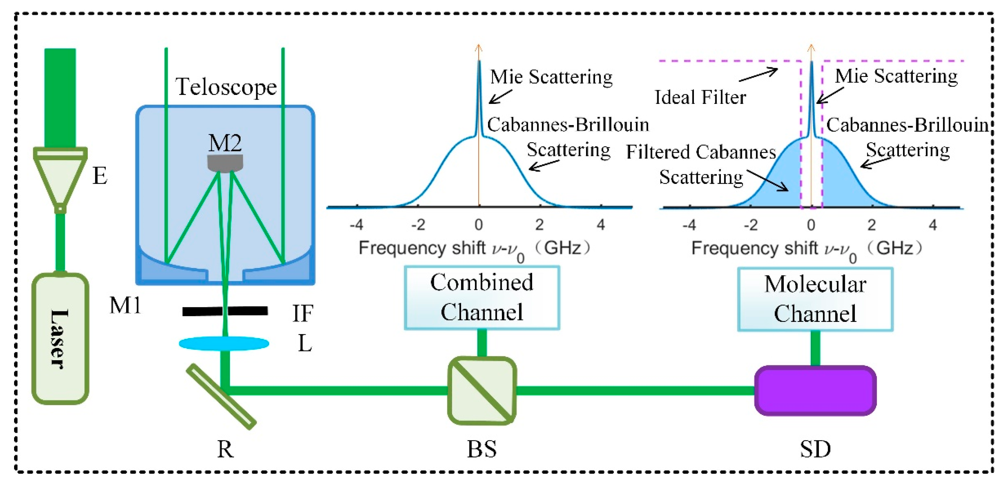
2.1. The Basic HSRL Theory
2.2. The Noise Model in HSRL
2.3. Standard Method
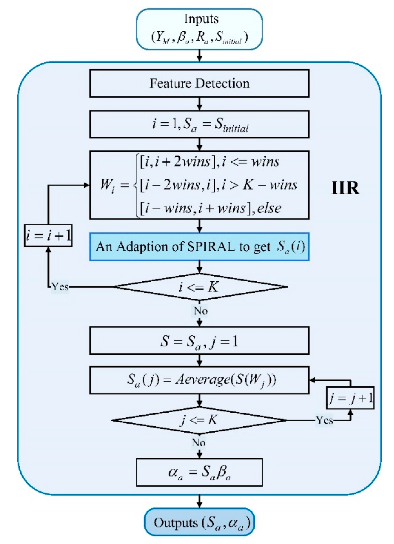
2.4. Iterative Image Reconstruction (IIR) Method
3. Error Analysis Based on Monte-Carlo Simulations
3.1. The Specifications of MC Simulations
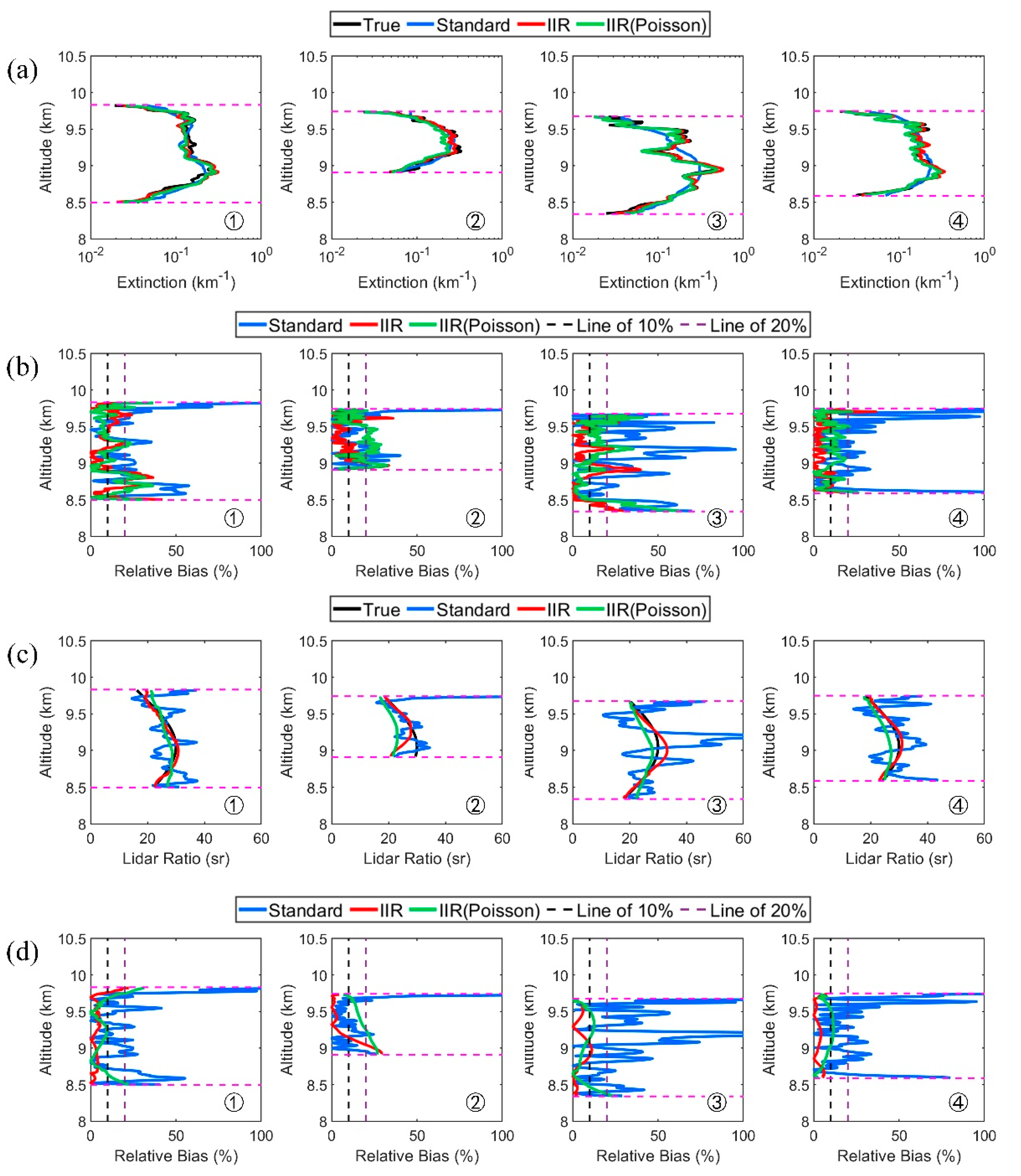
3.2. Comparison Between the Standard Method and IIR Method
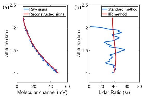
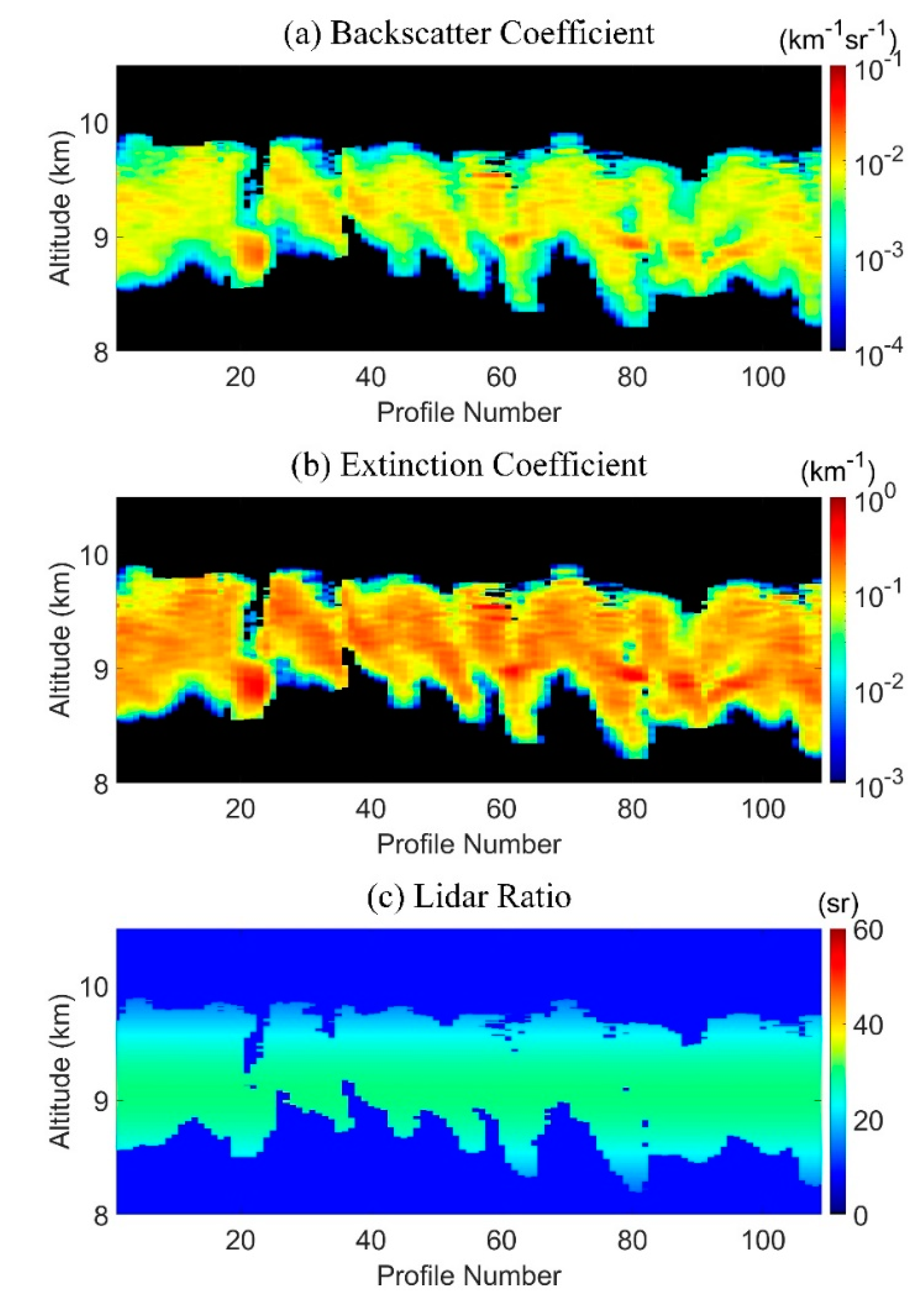
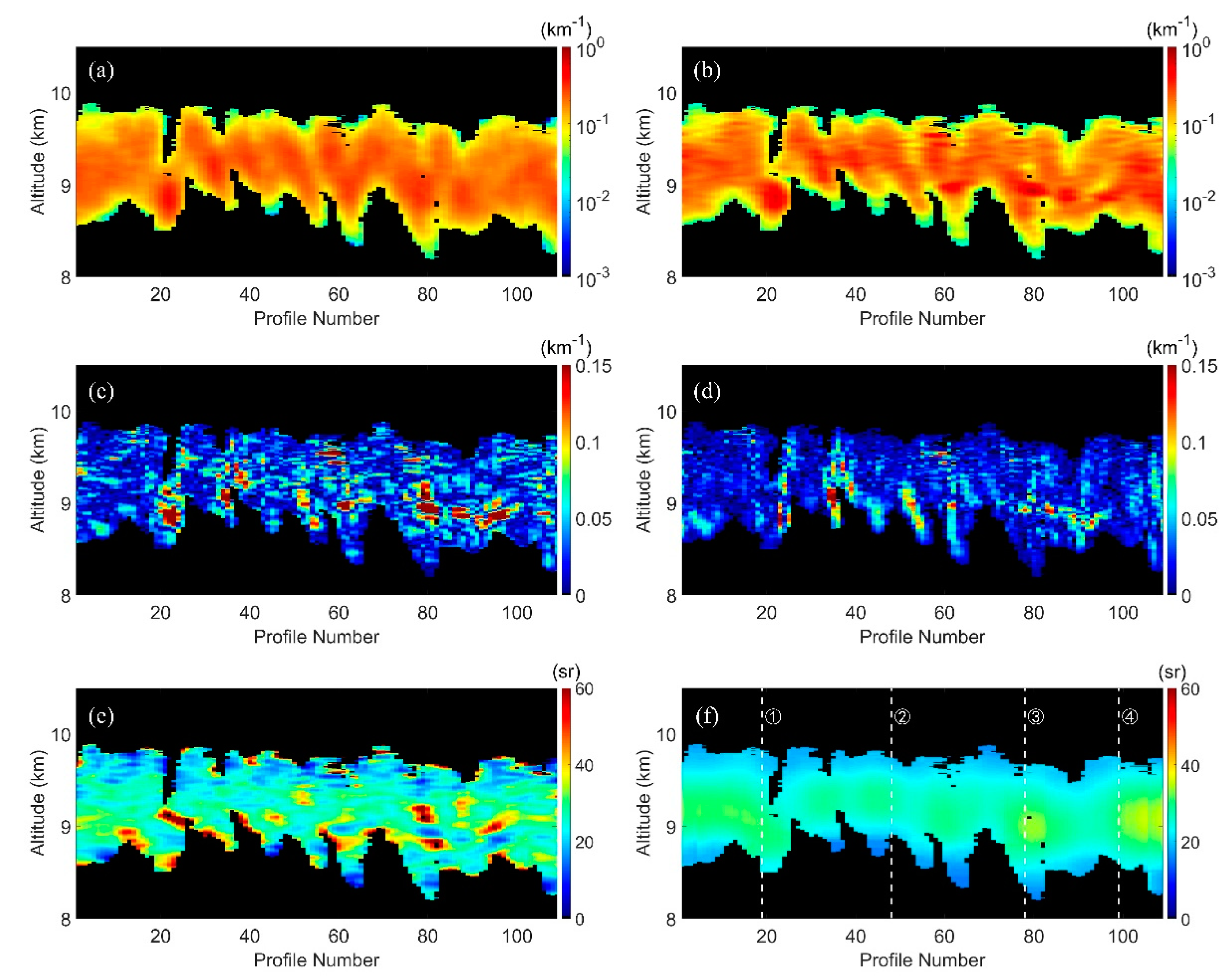
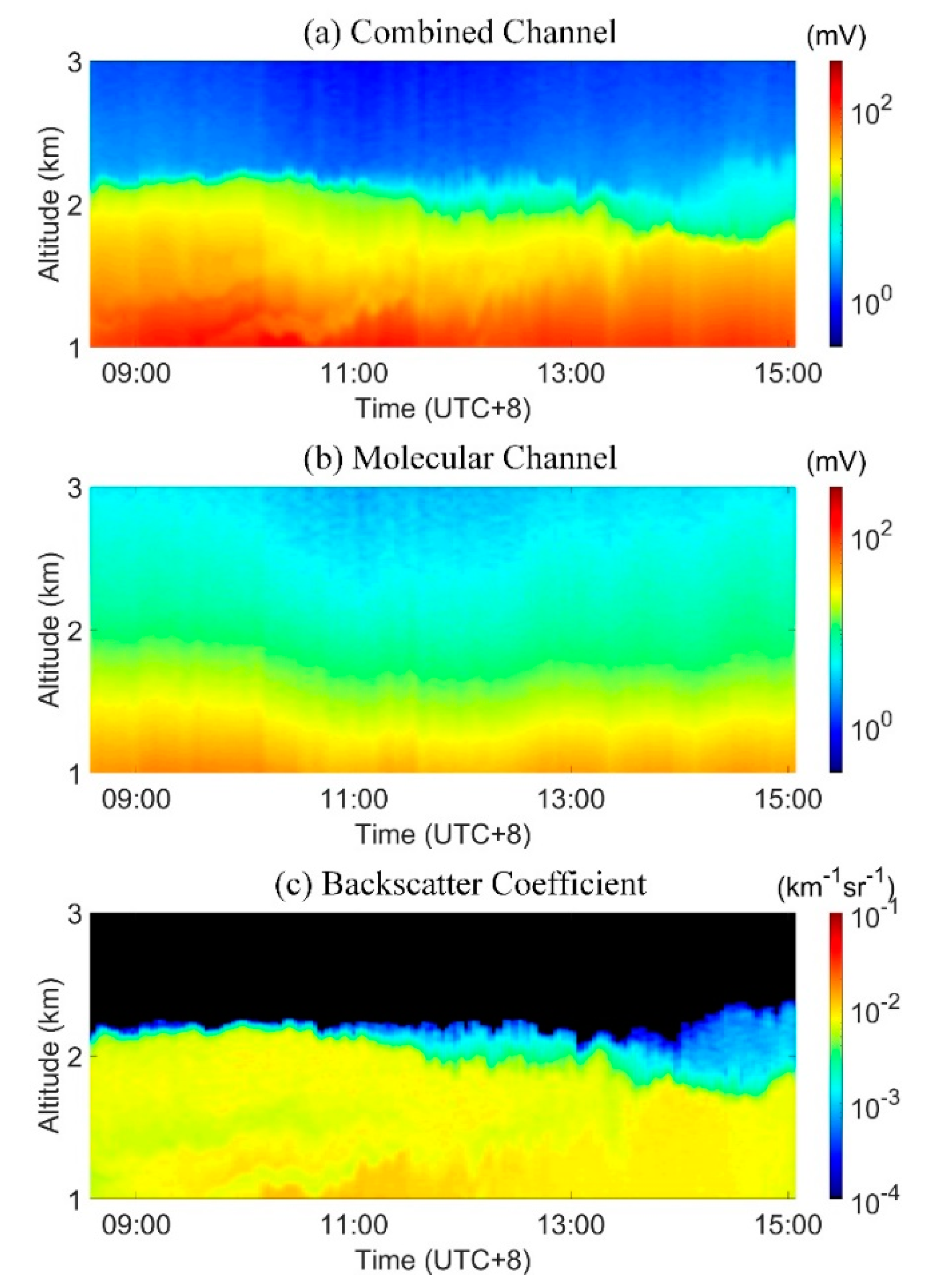
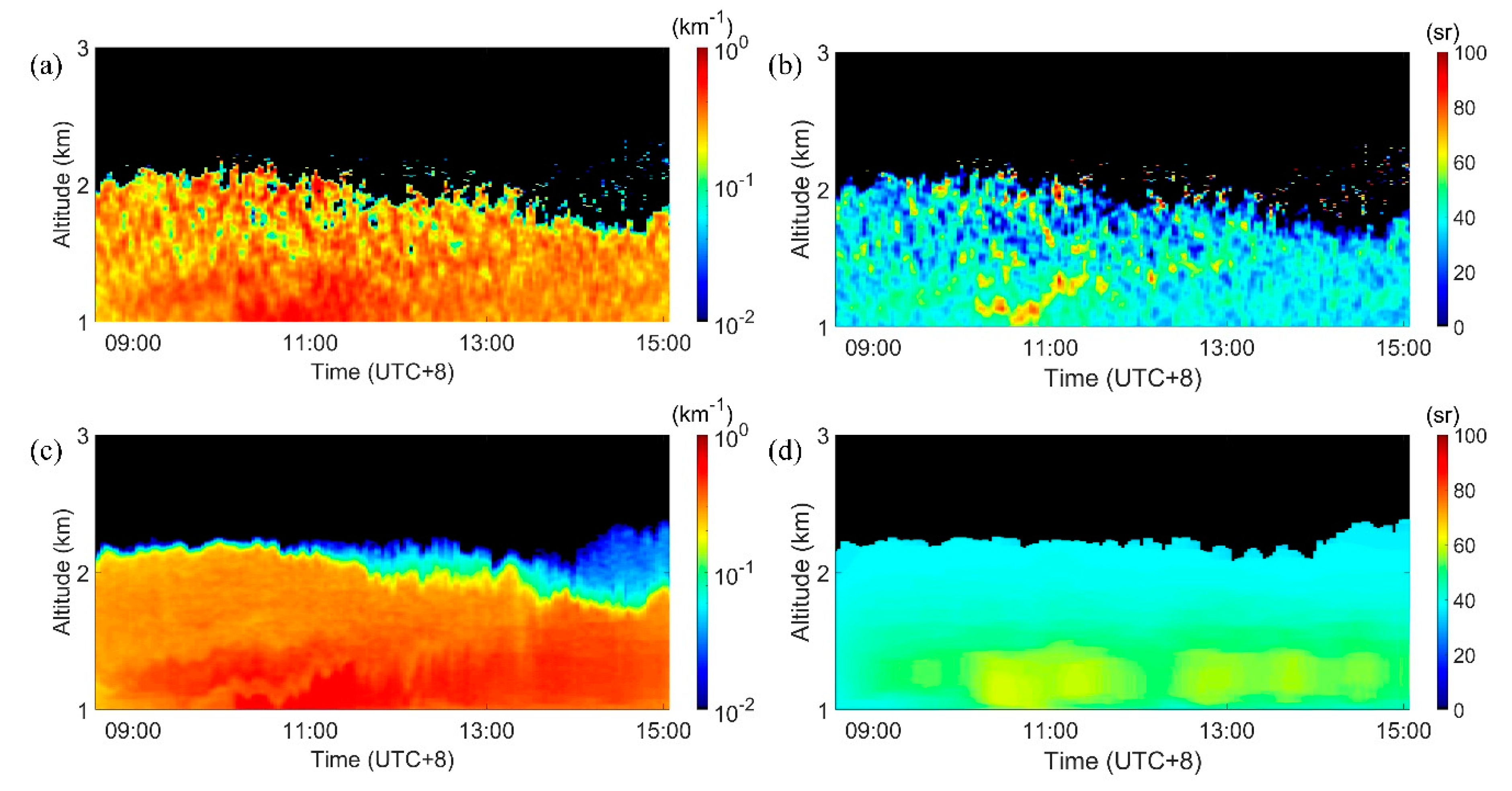
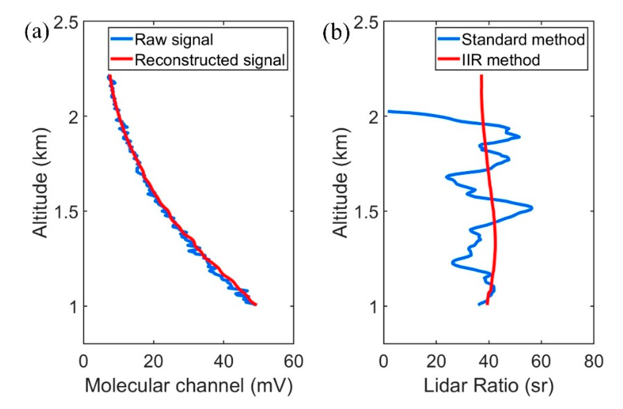
4. Results
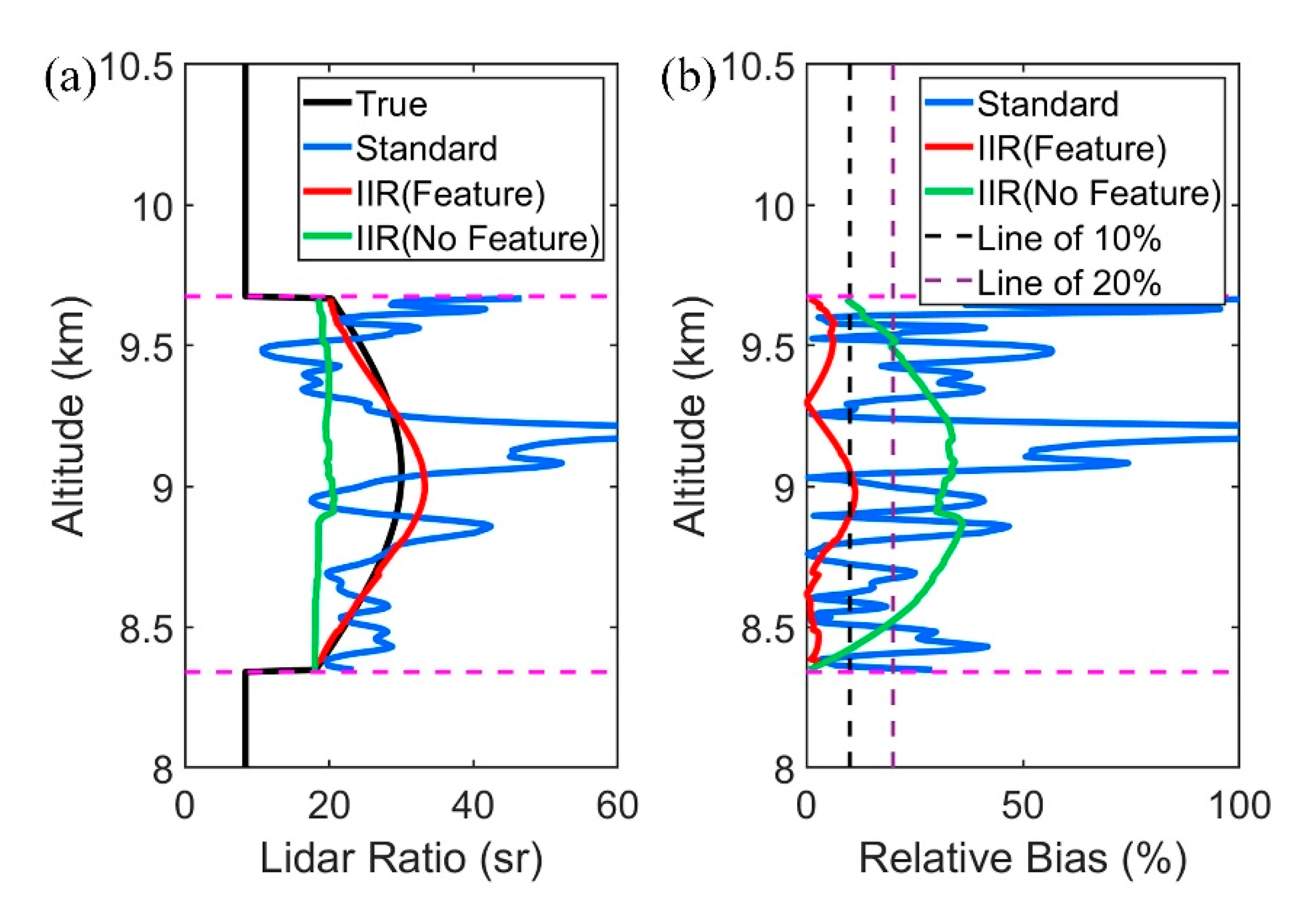
5. Discussion
6. Conclusions
Author Contributions
Funding
Acknowledgments
Conflicts of Interest
References
- Solomon, S.D.; Qin, D.; Manning, M.; Chen, Z.; Marquis, M.; Avery, K.; Miller, H. Climate Change 2007: The Physical Science Basis. Working Group I Contribution to the Fourth Assessment Report of the IPCC. Available online: https://www.google.com.hk/url?sa=t&rct=j&q=&esrc=s&source=web&cd=&cad=rja&uact=8&ved=2ahUKEwiwuNvn4fHrAhUGq5QKHdrTABUQFjACegQIBBAB&url=https%3A%2F%2Fwww.ipcc.ch%2Fsite%2Fassets%2Fuploads%2F2018%2F02%2Far4-wg1-frontmatter-1.pdf&usg=AOvVaw1MGSugu1rfFBiMKOeBC8ey (accessed on 20 June 2020).
- Mattis, I.; D’Amico, G.; Baars, H.; Amodeo, A.; Madonna, F.; Iarlori, M. EARLINET Single Calculus Chain – technical—Part 2: Calculation of optical products. Atmos. Meas. Tech. 2016, 9, 3009–3029. [Google Scholar] [CrossRef] [Green Version]
- Böckmann, C.; Wandinger, U.; Ansmann, A.; Bösenberg, J.; Amiridis, V.; Boselli, A.; Delaval, A.; De Tomasi, F.; Frioud, M.; Grigorov, I.; et al. Aerosol lidar intercomparison in the framework of the EARLINET project. 2. Aerosol backscatter algorithms. Appl. Opt. 2004, 43, 977–989. [Google Scholar] [CrossRef] [PubMed]
- Li, Y.; Wang, B.; Lee, S.-Y.; Zhang, Z.; Wang, Y.; Dong, W. Micro-Pulse Lidar Cruising Measurements in Northern South China Sea. Remote Sens. 2020, 12, 1695. [Google Scholar] [CrossRef]
- Chan, P.W. Determination of Backscatter-Extinction Coefficient Ratio for LIDAR-Retrieved Aerosol Optical Depth Based on Sunphotometer Data. Remote Sens. 2010, 2, 2127. [Google Scholar] [CrossRef] [Green Version]
- Eloranta, E.E. High Spectral Resolution Lidar. In Lidar: Range-Resolved Optical Remote Sensing of the Atmosphere; Weitkamp, C., Ed.; Springer: New York, NY, USA, 2005; pp. 143–163. [Google Scholar]
- Liu, D.; Yang, Y.; Cheng, Z.; Huang, H.; Zhang, B.; Ling, T.; Shen, Y. Retrieval and analysis of a polarized high-spectral-resolution lidar for profiling aerosol optical properties. Opt. Express 2013, 21, 13084–13093. [Google Scholar] [CrossRef] [PubMed]
- Hair, J.W.; Hostetler, C.A.; Cook, A.L.; Harper, D.B.; Ferrare, R.A.; Mack, T.L.; Welch, W.; Izquierdo, L.R.; Hovis, F.E. Airborne High Spectral Resolution Lidar for profiling aerosol optical properties. Appl. Opt. 2008, 47, 6734–6752. [Google Scholar] [CrossRef]
- D’Amico, G.; Amodeo, A.; Mattis, I.; Freudenthaler, V.; Pappalardo, G. EARLINET Single Calculus Chain – technical—Part 1: Pre-processing of raw lidar data. Atmos. Meas. Tech. 2016, 8, 10387–10428. [Google Scholar] [CrossRef] [Green Version]
- Li, H.; Chang, J.; Xu, F.; Liu, Z.; Yang, Z.; Zhang, L.; Zhang, S.; Mao, R.; Dou, X.; Liu, B. Efficient Lidar Signal Denoising Algorithm Using Variational Mode Decomposition Combined with a Whale Optimization Algorithm. Remote Sens. 2019, 11, 126. [Google Scholar] [CrossRef] [Green Version]
- Eloranta, E. High Spectral Resolution Lidar Measurements of Atmospheric Extinction: Progress and Challenges. In Proceedings of the 2014 IEEE Aerospace Conference, Big Sky, MO, USA, 1–8 March 2014; pp. 1–6. [Google Scholar]
- Pornsawad, P.; D’Amico, G.; Böckmann, C.; Amodeo, A.; Pappalardo, G. Retrieval of aerosol extinction coefficient profiles from Raman lidar data by inversion method. Appl. Opt. 2012, 51, 2035–2044. [Google Scholar] [CrossRef]
- Mao, F.; Gong, W.; Li, C. Anti-noise algorithm of lidar data retrieval by combining the ensemble Kalman filter and the Fernald method. Opt. Express 2013, 21, 8286. [Google Scholar] [CrossRef]
- Raghunath, K.; Sarvani, M.; Rao, S. Lidar signal denoising methods- application to NARL Rayleigh lidar. J. Opt. (India) 2015, 44, 164–171. [Google Scholar] [CrossRef]
- Song, Y.; Zhou, Y.; Liu, P.; Shi, G.; Wang, Y.; Di, H.; Hua, D. Research on an adaptive filter for the Mie lidar signal. Appl. Opt. 2019, 58, 62–68. [Google Scholar] [CrossRef] [PubMed]
- Zhou, Z.; Hua, D.; Wang, Y.; Yan, Q.; Li, S.; Li, Y.; Wang, H. Improvement of the signal to noise ratio of Lidar echo signal based on wavelet de-noising technique. Opt. Lasers Eng. 2013, 51, 961–966. [Google Scholar] [CrossRef]
- Pappalardo, G.; Amodeo, A.; Pandolfi, M.; Wandinger, U.; Wang, X. Aerosol Lidar Intercomparison in the Framework of the EARLINET Project. 3. Raman Lidar Algorithm for Aerosol Extinction, Backscatter, and Lidar Ratio. Appl. Opt. 2004, 43, 5370–5385. [Google Scholar] [CrossRef]
- Esselborn, M.; Wirth, M.; Fix, A.; Tesche, M.; Ehret, G. Airborne high spectral resolution lidar for measuring aerosol extinction and backscatter coefficients. Appl. Opt. 2008, 47, 346–358. [Google Scholar] [CrossRef]
- Marais, W.J.; Holz, R.E.; Hu, Y.H.; Kuehn, R.E.; Eloranta, E.E.; Willett, R.M. Approach to simultaneously denoise and invert backscatter and extinction from photon-limited atmospheric lidar observations. Appl. Opt. 2016, 55, 8316–8334. [Google Scholar] [CrossRef]
- Liu, Z.; Sugimoto, N. Simulation study for cloud detection with space lidars by use of analog detection photomultiplier tubes. Appl. Opt. 2002, 41, 1750–1759. [Google Scholar] [CrossRef]
- Wang, N.; Shen, X.; Xiao, D.; Veselovskiy, I.; Zhao, C.; Chen, F.; Liu, C.; Rong, Y.; Ke, J.; Wang, B.; et al. Development of ZJU High-spectral-resolution Lidar for Aerosol and Cloud: Feature Detection and Classification. J. Quant. Spectrosc. Ra. 2020. under review. [Google Scholar]
- Liu, D.; Hostetler, C.; Miller, I.; Cook, A.; Hair, J. System analysis of a tilted field-widened Michelson interferometer for high spectral resolution lidar. Opt. Express 2012, 20, 1406–1420. [Google Scholar] [CrossRef]
- Cheng, Z.; Liu, D.; Zhang, Y.; Yang, Y.; Zhou, Y.; Luo, J.; Bai, J.; Shen, Y.; Wang, K.; Liu, C.; et al. Field-widened Michelson interferometer for spectral discrimination in high-spectral-resolution lidar: Practical development. Opt. Express 2016, 24, 7232–7245. [Google Scholar] [CrossRef]
- Liu, D.; Zheng, Z.; Chen, W.; Wang, Z.; Li, W.; Ke, J.; Zhang, Y.; Chen, S.; Cheng, C.; Wang, S. Performance estimation of space-borne high-spectral-resolution lidar for cloud and aerosol optical properties at 532 nm. Opt. Express 2019, 27, A481–A494. [Google Scholar] [CrossRef] [PubMed]
- Liu, Z.; Hunt, W.; Vaughan, M.; Hostetler, C.; McGill, M.; Powell, K.; Winker, D.; Hu, Y. Estimating random errors due to shot noise in backscatter lidar observations. Appl. Opt. 2006, 45, 4437–4447. [Google Scholar] [CrossRef] [PubMed]
- Shcherbakov, V. Regularized algorithm for Raman LIDAR data processing. Appl. Opt. 2007, 46, 4879–4889. [Google Scholar] [CrossRef]
- Harmany, Z.T.; Marcia, R.F.; Willett, R.M. This is SPIRAL-TAP: Sparse Poisson Intensity Reconstruction ALgorithms—Theory and Practice. IEEE Trans. Image Process. 2012, 21, 1084–1096. [Google Scholar] [CrossRef] [Green Version]
- Liu, D.; Shi, T.; Zhang, L.; Yang, Y.; Chong, S.; Shen, Y. Reverse optimization reconstruction of aspheric figure error in a non-null interferometer. Appl. Opt. 2014, 53, 5538–5546. [Google Scholar] [CrossRef]
- Cheng, Z.; Liu, D.; Luo, J.; Yang, Y.; Su, L.; Yang, L.; Huang, H.; Shen, Y. Effects of spectral discrimination in high-spectral-resolution lidar on the retrieval errors for atmospheric aerosol optical properties. Appl. Opt. 2014, 53, 4386–4397. [Google Scholar] [CrossRef] [PubMed]
- Oh, A.K.; Harmany, Z.T.; Willett, R.M. Logarithmic total variation regularization for cross-validation in photon-limited imaging. In Proceedings of the IEEE International Conference on Image Processing, Melbourne, VIC, Australia, 15–18 September 2013; pp. 484–488. [Google Scholar]
- Veselovskii, I.; Kolgotin, A.; Griaznov, V.; Müller, D.; Wandinger, U.; Whiteman, D.N. Inversion with regularization for the retrieval of tropospheric aerosol parameters from multiwavelength lidar sounding. Appl. Opt. 2002, 41, 3685–3699. [Google Scholar] [CrossRef] [Green Version]
- Beck, A.; Teboulle, M. Fast Gradient-Based Algorithms for Constrained Total Variation Image Denoising and Deblurring Problems. IEEE Trans. Image Process. 2009, 18, 2419–2434. [Google Scholar] [CrossRef] [Green Version]
- Tao, Z.; Liu, D.; Zhong, Z.; Shi, B.; Nie, M.; Ma, X.; Zhou, J. Effective Lidar Ratio of Cirrus Cloud Measured by Three-Wavelength Lidar. Chin. J. Lasers 2016, 43, 0810003. [Google Scholar]
- Wang, J.; Liu, W.; Liu, C.; Liu, J.; Chen, Z.; Xiang, Y.; Meng, X. The Determination of Aerosol Distribution by a No-Blind-Zone Scanning Lidar. Remote Sens. 2020, 12, 626. [Google Scholar] [CrossRef] [Green Version]
- Shen, X.; Liu, D.; Wang, N.; Xiao, D.; Rong, Y.; Zhong, T.; Liu, C.; Zhang, K.; Zhou, Y.; Chen, S. Development of ZJU High-spectral-resolution Lidar for Aerosol and Clouds: Calibration of Overlap Function. J. Quant. Spectrosc. Ra. 2020. under review. [Google Scholar]
- Müller, D.; Ansmann, A.; Mattis, I.; Tesche, M.; Wandinger, U.; Althausen, D.; Pisani, G. Aerosol-type-dependent lidar ratios observed with Raman lidar. J. Geophys. Res. 2007, 112, D16202. [Google Scholar] [CrossRef]
- Xie, C.; Nishizawa, T.; Sugimoto, N.; Matsui, I.; Wang, Z. Characteristics of aerosol optical properties in pollution and Asian dust episodes over Beijing, China. Appl. Opt. 2008, 47, 4945–4951. [Google Scholar] [CrossRef] [PubMed]
- Ruijun, D.; Yang, Y.; Li, H.; Hu, F.; Wang, Z.; Huang, Z.; Zhou, T.; Zhang, T. Atmosphere Boundary Layer Height (ABLH) Determination under Multiple-Layer Conditions Using Micro-Pulse Lidar. Remote Sens. 2019, 11, 263. [Google Scholar] [CrossRef] [Green Version]
- Zhong, T.; Wang, N.; Shen, X.; Xiao, D.; Xiang, Z.; Liu, D. Determination of Planetary Boundary Layer height with Lidar Signals Using Maximum Limited Height Initialization and Range Restriction (MLHI-RR). Remote Sens. 2020, 12, 2272. [Google Scholar] [CrossRef]


| Specifications | Value |
|---|---|
| Laser wavelength (nm) | 532 |
| Laser energy (mJ) | 200 |
| Diameter of primary telescope (mm) | 280 |
| Interference filter bandpass (nm) | 0.3 |
| Range resolution (m) | 7.5 |
| Temporal resolution (s) | 10 |
| Molecular transmittance of spectral discrimination filter | 0.19 |
| Aerosol transmittance of spectral discrimination filter (e-12) | 2.52 |
| Type of noise | Gaussian |
| Extinction | RMSE | Relative bias |
| Standard method | 0.015 | 0.285 |
| IIR method | 0.009 | 0.170 |
| IIR method (Poisson) | 0.010 | 0.176 |
| Lidar Ratio | RMSE | Relative bias |
| Standard method | 2.451 | 0.226 |
| IIR method | 0.870 | 0.085 |
| IIR method (Poisson) | 0.950 | 0.105 |
© 2020 by the authors. Licensee MDPI, Basel, Switzerland. This article is an open access article distributed under the terms and conditions of the Creative Commons Attribution (CC BY) license (http://creativecommons.org/licenses/by/4.0/).
Share and Cite
Xiao, D.; Wang, N.; Shen, X.; Landulfo, E.; Zhong, T.; Liu, D. Development of ZJU High-Spectral-Resolution Lidar for Aerosol and Cloud: Extinction Retrieval. Remote Sens. 2020, 12, 3047. https://doi.org/10.3390/rs12183047
Xiao D, Wang N, Shen X, Landulfo E, Zhong T, Liu D. Development of ZJU High-Spectral-Resolution Lidar for Aerosol and Cloud: Extinction Retrieval. Remote Sensing. 2020; 12(18):3047. https://doi.org/10.3390/rs12183047
Chicago/Turabian StyleXiao, Da, Nanchao Wang, Xue Shen, Eduardo Landulfo, Tianfen Zhong, and Dong Liu. 2020. "Development of ZJU High-Spectral-Resolution Lidar for Aerosol and Cloud: Extinction Retrieval" Remote Sensing 12, no. 18: 3047. https://doi.org/10.3390/rs12183047