The Global Wind Resource Observed by Scatterometer

Abstract

A 27-year-long calibrated multi-mission scatterometer data set is used to determine the global basin-scale and near-coastal wind resource. In addition to mean and percentile values, the analysis also determines the global values of both 50- and 100-year return period wind speeds. The analysis clearly shows the seasonal variability of wind speeds and the differing response of the two hemispheres. The maximum wind speeds in each hemisphere are comparable but there is a much larger seasonal cycle in the northern hemisphere. As a result, the southern hemisphere has a more consistent year-round wind climate. Hence, coastal regions of southern Africa, southern Australia, New Zealand and southern South America appear particularly suited to coastal and offshore wind energy projects. The extreme value analysis shows that the highest extreme wind speeds occur in the North Atlantic Ocean with extreme wind regions concentrated along the western boundaries of the North Atlantic and North Pacific Oceans and the Indian Ocean sector of the Southern Ocean. The signature of tropical cyclones is clearly observed in each of the well-known tropical cyclone basins.

1. Introduction

The determination of the global offshore wind energy resource and the design and operation of coastal and offshore wind energy projects require long-term measurements of wind conditions. There are a variety of systems which can be used to provide such information, including: in situ anemometer data, remote sensing applications, and numerical modelling. Anemometer records obviously provide a direct measurement at the location of interest, but they are limited to specific areas and long-term records are seldom available at locations of interest. Satellite systems such as altimeters, radiometers and scatterometers have the advantage that they provide global coverage and the data record for each of these systems is now approximately 30 years. Numerical models have clearly advanced in terms of their accuracy and resolution, but they still require validation against actual measurements.

A number of previous studies have used an altimeter, radiometer and scatterometer measurements to assess global climatology of wind speed and wave height [1,2,3,4]. These studies have generally used relatively short satellite records (decade) for these studies. The advent of long-term databases of multiple-mission satellite data for altimeter [4,5,6], radiometer [7] and scatterometer [8] provides the opportunity to examine both the climatology and extreme value global distribution of wind speed. Each of these satellite systems has similar error statistics [9], however, the sampling pattern of altimeters and the degradation of radiometer measurements in heavy rain mean that scatterometers are the preferred instrument for the measurement of global-scale wind speed.

The present paper uses a long-term consistently calibrated and validated archive of scatterometer data compiled over a 27-year period [8] to investigate global wind climatology and extreme value (1 in 50- and 100-year) wind speed estimates. In addition, the data are processed to obtain the distribution of wind speeds along coastlines, thus making it directly applicable as a resource for the offshore wind energy industry.

The arrangement of the paper is as follows. Following this introduction, Section 2 provides an overview of scatterometer measurement of wind speed, the datasets and the methods used to estimate climatologic values and extremes values. Section 3 describes both the ocean-scale basin and coastline analyses of the data. This is followed by a discussion of the results in Section 4 and conclusions in Section 5.

2. Materials and Methods

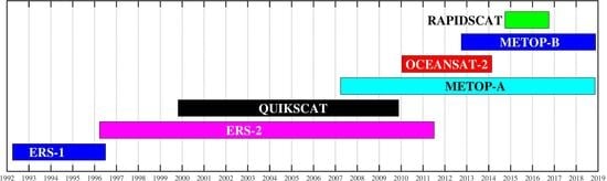
2.1. Scatterometer Wind Speed Measurement

Scatterometers (like altimeters) are “active” sensors in that they transmit a microwave radar signal to the water surface and monitor the received energy. In contrast, radiometers are “passive” sensors in that they monitor radiation emanating naturally from the water surface. The transmitted energy is reflected from the water surface as a result of Bragg scattering [10]. Bragg scattering is constructive interferences between the transmitted wave and the surface water waves. Water waves with a wavelength ${\lambda }_w=\lambda /(2\cos \theta )$ satisfy the Bragg resonance conditions, where $\lambda$ is the microwave scatterometer wavelength and $\theta$ is the incident angle of the scatterometer energy on the water surface. Scatterometers typically operate in either the C-band (5.255 GHz) or the Ku-band (13.4 GHz), for which the microwave wavelengths are 5 and 2 cm, respectively. Hence, the wavelengths of the Bragg scattering water waves, $\lambda$ are of order centimetres. These short centimetre-scale waves respond almost instantaneously to the local wind and hence the Bragg scattering provides a means of indirectly sensing the wind speed.

The radar cross-section, ${\sigma }_0$ is defined as the ratio of the received power at the satellite antenna to the transmitted power. The radar cross-section, ${\sigma }_0$, can be related to the neutral stability wind speed, measured at an elevation of 10 m, $U_{10}$ and the wind direction, $\varphi$ through a Geophysical Model Function (GMF), ${\sigma }_0=GMF(U_{10},\theta ,\varphi ,\rho ,\lambda )$, where $\rho$ is the radar polarization [11,12,13,14]. There are two unknowns in this relationship, the wind speed, $U_{10}$ and wind direction, $\varphi$. In addition, it is necessary to resolve the 180-degree wind direction ambiguity. Hence, a minimum of three measurements of the radar cross-section is required at each location. Multiple measurements (often more than three) are obtained by having an antenna configuration which can image the same location at different angles. There is a wide range of both fan and pencil beam scatterometer antenna designs which achieve these requirements, whilst measuring over a broad swath [8].

As noted above, $U_{10}$ is the wind velocity at a reference height of 10 m for a neutral stability boundary layer. That is, a marine boundary layer for which the air and water temperatures are equal. In such a case, the boundary layer follows a logarithmic form [15,16,17]. If the water temperature is greater than the air temperature, then there is cold air overlaying warm air and hence density differences result in a vertical circulation. In this case, the boundary layer is described as unstable and there is a more uniform distribution of wind speed with height than represented by the logarithmic form. Conversely, if the water temperature is less than the air temperature, there is warm air overlaying cold air and the boundary layer is described as stable. In this case, the velocity profile varies more rapidly with height than described by the logarithmic profile [7]. Such stability effects have an influence on wind speed measurements and predictions over the ocean, irrespective of the data source. For instance, estimations of wind speeds at a reference height (usually 10 m) are impacted irrespective of whether they come from models, anemometers or remote sensing systems.

In the case of remote sensing measurements, including scatterometers, as described above, short-wavelength waves are being used as a proxy for wind speed. These short waves respond to the wind speed at a height comparable to their wavelengths, which are very short [7]. The calibration process used for such instruments [8] relates the radar backscatter ${\sigma }_0$ to anemometer data at a reference height of 10 m. As these data very commonly come from buoy mounted instruments at heights less than 10 m, they are corrected to a height of 10 m using the assumption of a neutrally stable logarithmic boundary layer. As such neutral conditions occur rarely over the world’s oceans [7], this process introduces some error. As the calibrations are, however, carried out across many different buoys and over many years, a broad range of conditions is encountered. Hence, it is commonly assumed that such stability effects are averaged out in the calibration. Because of its long duration and number of buoys far from land, the NDBC buoy network [18] around the United States coastline is typically used for such calibrations. As shown by Young and Donelan [7], in the context of altimeter and radiometer, when such calibrations are applied to other geographic locations, with larger stability effects, they can result in a bias in the data. Although such detailed comparisons have not been undertaken for scatterometer, as the frequency of operation is similar to the altimeter, the impacts should be comparable. The stability impact of the altimeter is a function of air–water temperature difference and wind speed [7]. For a temperature difference of 2 °C and a wind speed of 5 ms⁻¹, the error is approximately 10%. This percentage error increases as the wind speed decreases and the temperature difference increases.

Noting that the mechanism used by scatterometers, and other remote sensing systems, to measure wind speed relies on the use of short-scale waves on the water surface as a proxy for the wind speed, such systems only measure wind speeds over the oceans (not land).

2.2. Scatterometer Database

Ribal and Young [8] have compiled a long-term database of duration 27-years (1992 to 2019) of scatterometer data. The data includes the satellite missions ERS-1, ERS-2, QUIKSCAT, METOP-A, OCEANSAT-2, METOP-B and RAPIDSCAT. Each scatterometer was independently calibrated against NDBC buoy data [18] and validated against other scatterometers in orbit at the same time at cross-over locations. In addition, as the performance of buoy anemometers is questionable at high wind speeds due to ocean wave sheltering [19,20,21,22,23], Ribal and Young [8] calibrated the scatterometers for wind speeds above 25 ms⁻¹ using platform data.

Scatterometers are typically placed in near-polar sun-synchronous orbits (with the exception of RAPIDSCAT). The instrument measures over a swath varying in width between 1000 and 1500 km and with a spatial resolution of 25 km in both along-track and cross-track directions. As a result, a single scatterometer will image almost the full surface of the earth (between latitudes of ±80°) twice per day. As shown in Figure 1, for much of the period of the available data, there were multiple scatterometers in orbit. As a result, each location around the globe is imaged multiple times per day. As such, there are generally sufficient observations to form accurate monthly statistics for mean and percentile wind speed [7] as well as defining the tail of the probability distribution function for extreme value analysis [24].

The Ribal and Young [8] calibrations of the scatterometer systems used large co-location datasets (typically greater than 50,000 for each scatterometer) with buoy data. These calibrations produced typical error statistics between the scatterometer and buoy of the root mean square error, $RMSE\approx 1.0$ ms⁻¹ and $\left|Bias\right|\approx 0.1$ ms⁻¹. In a triple co-location study involving scatterometer, altimeter, radiometer and buoys [9], scatterometers were shown to have error standard deviations of approximately 0.5 ms⁻¹. Interestingly, this was actually smaller than buoy mounted anemometers, 0.8 ms⁻¹. These error statistics are consistent with a range of other similar studies [25,26,27,28,29,30]. As a result of the consistent error statistics for scatterometers, they have largely become the reference for large-scale model validation of wind speeds over the oceans [31].

2.3. Climatology

In order to form stable monthly statistics, the data were binned into 2° × 2° bins and the monthly mean (${\overline{U}}_{10}$) and the monthly 10th ($U_{10}(10)$), 70th ($U_{10}(70)$), 90th ($U_{10}(90)$) and 99th ($U_{10}(99)$) percentiles determined for each bin [1,2,7], where $U_{10}$ is the scatterometer calibrated wind speed at an elevation of 10 m.

2.4. Extreme Value Estimates

The aim of extreme value analysis (EVA) is to fit a theoretical probability distribution function (pdf) to a set of observations of events [32,33]. For the process to be valid, the data must satisfy two conditions. They must be independent and identically distributed (IID). As the focus of EVA is the distribution of the extreme tail of the distribution rather than the body of the pdf, independence can be interpreted as ensuring there are not multiple observations from the same storm. Unlike anemometer/buoy data, satellite data does not provide a time series at a fixed location where the passage of individual storms can be tracked. Hence, the requirement of independence is usually satisfied by ensuring a minimum time interval between observations. A value of 48 h has commonly been used [24,34,35,36] and is adopted here. The requirement that the data are identically distributed means that they should all be drawn from the same parent distribution. This requirement would not typically be satisfied where, for example, there are two or more independent meteorological systems which can generate extreme winds (e.g., tropical cyclones and trade winds). In such cases, the data should be partitioned, and the pdf of each partition determined separately [37]. The present dataset provides no mechanism to partition such data on a global scale. As a result, the present results may be limited in regions such as those where tropical cyclones dominate. Note such locations may also be impacted by the validity of the scatterometer data at high winds (see Section 4).

The application of EVA is typically aimed at determining the extreme wind speed associated with a defined probability of exceedance, $P_r$ or the return period $T_r=1/P_r$. As the length of the recorded time series of observations is very commonly shorter than the desired return period, EVA typically involves the fitting of a defined analytical pdf to the pdf of the observed extreme values and then extrapolating to the required probability level. Following Coles [33], there are two approaches which are commonly used to define the extreme value dataset and fit an appropriate analytical form: block maxima/annual maxima (AM) [33] and peaks over threshold (PoT) [34,38,39,40,41]. It can be shown [33,42] that for the AM method, in which the highest value in each year is selected, the resulting extreme value pdf will follow a generalized extreme value distribution. As only one value in each year is selected, the method ensures that the data are independent. The significant limitation of the method, however, is that, as only one value per year is selected, the pdf is typically constructed from only a limited number of data points (in the present case, 27 for the scatterometer data record). This results in considerable statistical sampling variability due to the small sample size. The PoT approach overcomes this limitation by selecting the peak value above a defined threshold, also ensuring there are no values separated by less than 48 h, as noted above. In such a case, it can be shown that the data will follow a generalized Pareto distribution (GPD) given by:

$$F(x)=1-\left[1+k{\left(\frac{x-A}{B}\right)}^{-1/k}\right]$$

(1)

where $F(x)$ is the pdf and $x$ is the variable under consideration (wind speed, $U_{10}$). In Equation (1), $A$ defines the threshold value, $B$ is a scale parameter and $k$ is a shape parameter. It is common to select a high percentile for the threshold, in this case, the 90th percentile [24,34,36,41,43,44,45]. With the theoretical pdf defined in this manner, it can be fitted to the observed data determining the best-fit parameters $B$ and $k$. The desired return period, in this case, the 100-year value is then defined as:

$$P_r(x<x^{100})=1-N_y/(100N_{PoT})$$

(2)

where $N_{PoT}$ is the number of data points in the PoT analysis and $N_y$ is the number of years spanned by the analysis.

As for the calculation of the climatology above, the data were binned into a 2° × 2° grid and both 50- and 100-year return period values of wind speed ($U_{10}^{50},U_{10}^{100}$) determined for each grid square. In order to validate the EVA described above, scatterometer values of $U_{10}^{100}$ were compared with deep water NDBC [18] buoy calculations using the same PoT analysis described above. The differences between buoy and scatterometer were quantified in terms of the relative error:

$$\Delta r=\left[U_{10}^{100}(Scat.)-U_{10}^{100}(Buoy)\right]/U_{10}^{100}(Buoy)$$

(3)

These values were then averaged across all buoys to obtain a mean error, $r$.

Table 1. Comparison of values of 100-year return period wind speed calculated using a PoT analysis for both scatterometer and NDBC deep-water buoys.

Buoy No.	Lat (°N), Lon(°E)	${\mathit{U}}_{10}^{100}\left(\mathbf{Buoy}\right)$ (ms−1)	${\mathit{U}}_{10}^{100}(\mathbf{Scat}.)$ (ms−1)
46001	56.23, 212.05	24.9	29.9
46002	42.61, 229.46	24.4	26.9
46003	51.33, 204.15	26.1	30.5
46005	46.14, 228.93	25.3	29.1
46006	40.78, 222.60	27.2	31.0
51005	24.42, 197.90	18.9	26.0
44004	38.48, 289.57	27.3	34.1
41002	31.76, 285.16	25.9	34.0
42001	25.90, 270.33	28.1	28.0
42002	26.09, 266.24	26.3	29.0
Error, $r$	-	-	15.2%

shows a comparison across the NDBC buoys. The scatterometer values of extreme wind speed are in reasonable agreement with the buoy data with a mean error of 15.2%. This value is quite similar to the results obtained by Takbash et al. [24] using altimeter derived wind speed data. It is interesting that the values of the scatterometer $U_{10}^{100}$ are consistently higher than the buoy data. This may be because extreme values calculated over a 2° × 2° region are not the same as a time series from a point location. That is, over the spatial region more storm peaks occur than at a point. This difference is considered further in Section 4.

2.5. Coastal Wind Speeds

As noted above, both the climatological and extreme values wind speeds were evaluated globally on a 2° × 2° grid. As our aim is to obtain representative values for coastlines, these values need to be associated with coastal segments. In order to do this, we have adopted the Dynamic Interactive Vulnerability Assessment database (DIVA) [46,47]. DIVA is a database for the assessment of coastal vulnerability at the global scale. The database, as such, is not used in this analysis, rather, we have adopted the 9866 DIVA coastal locations as appropriate points to define the near-coastal wind climate. Using a Geographical Information System (GIS) model, representative wind speed values (climatological and extreme) at each DIVA point were associated with the closest 2° grid point [47,48]. To ensure scatterometer microwave radar returns are not corrupted by the proximity to land, all data closer than 25 km from land were excluded from the analysis. As such, the coastal values reported are characteristic of the open ocean conditions offshore from the coast.

3. Results

3.1. Ocean Basin Analysis

Figure 2 and Figure 3 show the mean monthly (${\overline{U}}_{10}$) and monthly 99th percentile ($U_{10}(99)$) wind speeds, respectively, colour contoured globally. The major climatological features previously reported from model and altimeter wind speed climatology [1,7] are apparent. The zonal variation of wind speeds is clear with the strongest wind speeds evident at high latitudes in winter in both hemispheres. The magnitudes of the mean winter wind speeds (Figure 2, January, July) at high latitudes ($\sim$12 ms⁻¹) in both hemispheres are comparable. The strongest mean winds are concentrated in the North Atlantic (Figure 2, January) and the Indian Ocean basin of the Southern Ocean (Figure 2, July). The summer comparison between the hemispheres at high latitudes are quite different from the North Atlantic decreasing significantly to $\sim$8.5 ms⁻¹, whilst the Southern Ocean decreases to only $\sim$10.5 ms⁻¹. That is, the Northern hemisphere has a much larger seasonal variation whilst the Southern Ocean experiences strong mean winds year-round. The North Atlantic experiences slightly stronger mean wind speeds than the North Pacific in both summer and winter.

The other striking feature of the distribution of ocean basin-scale wind speeds are the strong trade wind belts in the mid-latitudes of both hemispheres, which exist across all major ocean basins (Figure 2). Compared to higher latitudes, the trade wind belts are persistent for most of the year at mean wind speeds of $\sim$8 ms⁻¹. There are also a number of local features such as the strong localized mean wind speeds associated with the Somali jet in the Arabian Sea in June, July, August (Figure 2), associated with the onset of the Monsoon. Clear wind shadows are also seen east of New Zealand and South America (April to November Figure 2), where the strong westerly winds are blocked by the high mountain ranges.

The 99th percentile wind speeds, ($U_{10}(99)$) shown in Figure 3 indicate similar seasonal variations as the means. However, the trade winds are no longer apparent at these more extreme percentiles. That is, the trade winds are persistent year-round without being extreme. There is also a large triangularly shaped region at low latitudes in the southeastern Pacific where $U_{10}(99)$ is noticeably low, $\sim$10 ms⁻¹. The Somali jet which was prominent for ${\overline{U}}_{10}$ from June to August is no longer apparent for $U_{10}(99)$, indicating it is associated with consistent moderate winds but not extremes.

At these higher percentiles, the maximum wind speeds again occur in the respective winters of both hemispheres at high latitudes (Figure 3, January, July). Again, the southern hemisphere has a much smaller seasonal variation (extreme wind all year) than the northern hemisphere. Whereas the mean values were a maximum in the North Atlantic, the $U_{10}(99)$ maximum values are comparable across the North Atlantic, North Pacific and the Indian Ocean sector of the Southern Ocean ($\sim$22 ms⁻¹) (Figure 3, January, July).

Figures showing the distributions for the other percentiles are shown in the Supplementary Material (SM) ($U_{10}(10)$—Figure S1, $U_{10}(70)$—Figure S2, $U_{10}(90)$—Figure S3). The higher percentile cases are very similar to $U_{10}(99)$ (Figure 3). However, the spatial distributions of $U_{10}(10)$ (Figure S1) indicates that at this lower percentile the trade winds are now much more dominant. For significant, periods of the year the trade wind belts show the strongest winds globally at this lower percentile. This clearly demonstrates the differing structures of the wind speed pdfs in the trade winds compared to higher latitudes.

The global distribution of the 100-year return period wind speed $U_{10}^{100}$ is shown in Figure 4. The corresponding results for the 50-year return period are shown in the Supplementary Material (Figure S7). Figure 4 clearly shows greater statistical variability compared to the percentile plots above. This level of variability is consistent with previous studies of satellite extreme value estimates of wind speed and wave height [24,34,41] and is associated with the relatively large confidence limits resulting from the fitting of the GPD distribution Equation (1) to the data and extrapolating to the required probability of exceedance (Equation (2)) [24,43]. Both the magnitude and spatial distribution of $U_{10}^{100}$ are similar to that presented using a similar PoT analysis for altimeter data by Takbash et al. [24]. It is believed that this is the first time that scatterometer data has been processed to obtain such global extreme value estimates. The results have some similarities to the 99th percentile values (Figure 3), noting that the present results are effectivel for an even higher percentile. The maximum values are again generally associated with the higher latitudes of both hemispheres, with the maximum values occurring in the North Atlantic, followed by the North Pacific and the Southern Oceans. In both the North Atlantic and North Pacific, however, these regions of maximum values are displaced to the western side of the respective oceanic basins. This mirrors the tracks taken by storms in each of these basins. Atlantic hurricanes typically track across the Atlantic and either propagate into the Gulf of Mexico or turn north and follow the East Coast of the United States as they decay and often become higher latitude extra-tropical cyclones. The approximately triangular region in the eastern equatorial south Pacific previously noted for $U_{10}(99)$ (Figure 3) is again present for $U_{10}^{100}$ (Figure 4).

There are a number of regional maxima, all associated with tropical cyclone activity in Figure 4, which were not seen in the lower percentile estimates in Figure 3. These include the area between the Philippines and Japan in the South China Sea, associated with the highest density of tropical cyclone occurrence globally (typhoons) [24]. The signature of North American hurricanes is also seen east of Mexico and in the Gulf of Mexico. Further tropical cyclone related maxima are also present northwest of Australia, the Bay of Bengal and Madagascar.

An area of lower values of $U_{10}^{100}$ is located in the Indian Ocean west of Australia. This is an area where there is an unusually low density of tropical cyclone tracks [24]. There is also a region of large values of $U_{10}^{100}$ off the southeast coast of Australia. It is believed that this is associated with the occurrence of so-called “East Coast lows” in this region which results in intense storm conditions [49]. The enhanced spatial resolution of the scatterometer compared to altimeter means that these localized regions of extreme wind speeds are visible in the present EVA but have not been resolved in previous studies.

One area of note is the region of high winds identified in the Gulf of Guinea (West Africa). It is believed that these values are spurious and associated with a poor fit to the extreme value pdf (see Section 4).

3.2. Coastal Wind Climate

The coastal distributions of the mean month wind speed, ${\overline{U}}_{10}$, and 99th percentile monthly wind speed, $U_{10}(99)$ are shown in Figure 5 and Figure 6, respectively. Again, the 10th, 70th and 90th percentile values are shown in the SM ($U_{10}(10)$—Figure S4, $U_{10}(70)$—Figure S5, $U_{10}(90)$—Figure S6). The largest values of mean month wind speed (${\overline{U}}_{10}>10$ ms⁻¹) occur in the northern hemisphere winter along the East and West Coasts of Canada, the northeast coast of the United States, northern Europe and the coast of northern China and the Pacific coast of Russia. These results are consistent with the global distributions shown in Figure 2. With the exception of the southern tip of South America, southern hemisphere land masses are at lower latitudes than these regions in the northern Hemisphere, and hence experience lower mean monthly wind speeds than in the northern hemisphere.

As there is a much smaller seasonal variability in the southern hemisphere (Figure 2), however, the coastlines of southern Africa, southern Australia, New Zealand and southern South America experience values of ${\overline{U}}_{10}$ between 7 and 8 ms⁻¹ year-round. In contrast, the northern hemisphere locations mentioned above vary between less than 6 ms⁻¹ in summer and greater than 10 ms⁻¹ in winter. Hence, the southern hemisphere provides a potentially more consistent wind climate for offshore wind energy generation.

The trade wind belts which were so prominent in the global distributions (Figure 2) do not have a significant impact on mean monthly near-coastal wind speeds. Rather, there is a low latitude/high latitude distribution. In contrast to the higher latitudes, described above, lower latitudes ($\sim \pm$20°) have values of ${\overline{U}}_{10}<6$ ms⁻¹, year-round.

The 99th percentile wind speeds, $U_{10}(99)$ (Figure 6) show a very similar spatial distribution as for ${\overline{U}}_{10}$. The high latitude northern hemisphere regions (Canada, northeast US, northern Europe, China, Pacific coast of Russia) show $U_{10}(99)$ varying between 10 and 20 ms⁻¹ (summer to winter). In contrast, the high latitude southern hemisphere regions (southern Africa, southern Australia, New Zealand, southern South America) vary (summer to winter) between 14 to 17 ms⁻¹ for $U_{10}(99)$. The low latitude regions ($\sim \pm$20°) have values less than 10 ms⁻¹, year-round.

The 100-year return period near-coastal values, $U_{10}^{100}$ (Figure 7) show regions in excess 32 ms⁻¹ along the east coast of the United States, around Greenland, the Gulf of Mexico, the Bay of Bengal and South Africa. These same areas are also clear in the spatial distributions of Figure 4. Although Figure 4 shows very high values of $U_{10}^{100}$ in the South China Sea, the values near the coast in this region are lower, ranging from 24 to 28 ms⁻¹. As also seen in Figure 4, there is a relatively large percentage of the oceanic basins with values of $U_{10}^{100}$ between 20 to 28 ms⁻¹. In Figure 7, these areas occur down the east coast of the United States, the southern parts of South America, northern Europe, most of Asia, and most of Australia.

4. Discussion

The scatterometer data used in this study were selected for a number of reasons. Firstly, our desire is for a global assessment of the near-coastal wind resource, limiting consideration to either satellite or model data sources. Global wind models are now of high quality and certainly offer a valuable data resource. However, models are still limited by our understanding of the underlying physics and our ability to represent sub-grid scale influences. For this reason, we have opted for a satellite data source. Indeed, the present dataset represents a useful validation source for future model studies. Of the three potential global satellite data sources: altimeter, radiometer, scatterometer, all have some limitations. Altimeters measure only along a narrow beam at the satellite nadir. This means that, although the altimeter provides global coverage, the spatial resolution is limited, with altimeter tracks typically being separated by hundreds of kilometres [2,24,41]. Radiometers measure over a broad swath, eliminating the sampling constraint of altimeters. However, radiometer measurements are seriously degraded during rain events. As heavy rain events are often associated with strong winds, this constraint results in a “fair weather” bias for radiometer data. This limitation has been shown to make such data unusable for EVA [24]. In contrast, scatterometer data address both of these constraints, measuring over a broad swath and providing acceptable data in most rain events. Note, scatterometer data is degraded in heavy rain but not to the same magnitude as the radiometer. In addition, in triple collocation studies, it has been shown that the random errors in all three instruments are comparable and similar to buoys [9].

As noted above, global wind models have become common analysis and design tools and long-duration global reanalyses, such as ERA-Interim [50] and ERA5 [51] are commonly available. In order to assess the present composite scatterometer database against such reanalysis data, a comparison was made with the ERA5 dataset. ERA5 wind data is available at 0.25° resolution. These data were regretted to 2° resolution to make a comparison with the present scatterometer data. Rather than undertaking comparisons for every month as in Figure 2, both ERA5 and scatterometer data were averaged across the time period 1992 to 2019 and all months, to form annual average distributions of the 10 m elevation wind speed, $U_{10}$. Figure 8a,b shows the global distributions of these annual average values for scatterometer and ERA5, respectively. The spatial distributions of the major elements of the wind climatology are very similar between the two products. The strong zonal winds of the Southern Ocean, the strong winds of the North Atlantic and North Pacific and the distinct trade wind belts are all reproduced in both datasets. Figure 8c shows the difference between these results (${\overline{U}}_{10}(Scatt.)-{\overline{U}}_{10}(ERA5)$). A total of 75% of locations have an absolute difference less than 0.5 ms⁻¹. The major differences occur in the equatorial regions, the central South Pacific, the southern Indian Ocean, the eastern North Pacific and the East Coast of the United States where differences as high as 1 ms⁻¹ occur. Similar differences have been noted by Rivas and Stoffelen [31] when validating ERA-Interim and ERA5 against the ASCAT scatterometer. In this case, the differences were assumed to be limitations in the models’ ability to represent the impacts of ocean currents. However, Quilfen et al. [52] noted similar differences between buoy and ERS scatterometer data in the equatorial Pacific, indicating the issue may be regional scatterometer bias. As noted earlier, it has been shown that for the altimeter and radiometer, atmospheric boundary layer stability can result in regional variations in wind speed measurements [7].

To investigate the potential impact of atmospheric stability, the air–water temperature difference ($\Delta T=T_a-T_w$) is shown in Figure 8d. The values of $T_a$ and $T_w$ were obtained from the ERA-Interim archive. There is a remarkable degree of similarity between the wind speed difference (Figure 8c) and $\Delta T$ (Figure 8d). Many of the major ocean currents are clearly seen in this figure, including the Kuroshio current (Japan), the Gulf stream (East coast N. America) and the East Australian current. The warm waters across the equatorial regions are also clear. The high level of similarity between Figure 8c,d suggests that stability effects are important in describing the wind speed differences [7]. However, it is not possible to determine whether the scatterometer or ERA5 reanalysis is in error. It is likely that both datasets are impacted by these regional influences. Figure 8 provides a clear indication of the potential variability of boundary layer shape as a result of such global variations in air–water temperature differences. As pointed out by Young and Donelan [7], the vast majority of the world’s oceans experience unstable atmospheric conditions for most of the year.

There are also other limitations of the present data which are important to consider. Although scatterometer passes generally have a spatial resolution of 25 km, the present data have been binned at 2° resolution to form stable statistics (monthly means and percentiles and extreme value estimates). This is consistent with a range of previous studies [1,2,7,24,34,41]. In the present application, however, it means that the near-coastal values are representative of wind speeds, of order, 100 km offshore. Therefore, the results do not account for local influences which may change wind speeds closer to shore. Also, this resolution will not resolve local orographic effects.

The present analysis uses a multi-mission scatterometer database which has been extensively calibrated and validated against buoy and platform anemometer measurements. These calibrations are, however, limited to wind speeds up to 25 ms⁻¹. At higher wind speeds, the radar return for scatterometers begins to saturate, limiting accuracy and the validity of the calibration used [53,54,55]. As a result, there is reduced confidence in tropical cyclone regions and particularly, the EVA analysis for these locations. Despite this, the present results (Figure 4) yield EVA estimates in tropical cyclone regions which are consistent with design practice for such areas [56]. In addition, the present EVA results also show a range of local responses to tropical cyclones not previously apparent in either the lower resolution altimeter studies [24] or model estimates of such extremes [43].

Extreme value analyses such as that undertaken here are sensitive to the detailed shape of the measured pdf. In the present case, a GPD has been used to fit the observed data (Equation (1)). This functional form has three free parameters giving maximum flexibility in the fit. However, this can sometimes give rise to unrealistic fits to the data. For instance, the shape parameter $k$ can be either negative, resulting in a distribution with an upper bound, or positive resulting in an unbounded distribution. An example of such a poor fit to the data occurs in the Gulf of Guinea, where the GPD results in unrealistically large values of 100-year return period wind speeds, $U_{10}^{100}$. An alternative is to use a two-parameter exponential distribution in place of the GPD. However, the exponential distribution yields significantly higher values of $U_{10}^{100}$ which, unlike the GPD, are not in agreement with buoy data (Table 1).

The present EVA for the scatterometer data is consistent with buoy data (Table 1). However, the mean error across all locations is approximately 15%. In addition, at all but one location, the scatterometer yields larger extreme values. This result is very similar to that of Takbash et al. [24] for altimeter data. This suggests that the 2° × 2° binning used for these satellite datasets results in different extreme value statistics to a point buoy location. This is not surprising and suggests that more extreme events are identified by pooling the data over the spatial domain.

The climatologies in Figure 2 and Figure 3 represent averages over the period 1992 to 2019. Multiple studies have shown that over this period global mean wind speeds have changed as a result of multi-decadal oscillations and possibly anthropogenic global climate change. In a range of studies using both remote sensing and reanalysis data [57,58,59], it has been shown that the largest increases have occurred in the Southern Ocean. Over the period from 1985 to 2018 the average rate of wind speed increase in the Southern Ocean is approximately 2 cm⁻¹ yr⁻¹.

5. Conclusions

The present analysis uses a calibrated scatterometer multi-mission database of 27-years duration to examine the global near-coastal wind resource. The data were processed to determine the global climatology of monthly mean and percentile values and to present these both on an ocean-basin scale basis and around global coastlines. In addition, an extreme value analysis was undertaken to determine 100-year return period wind speeds across oceanic basins and at near-coastal sites.

The results clearly show the seasonal variations of wind speed across the globe. Of particular note is the different seasonal impacts in the different hemispheres. Both hemispheres have a maximum mean and percentile wind speeds in their respective winters at high latitudes. However, the northern hemisphere has a much larger variation between summer and winter than the southern hemisphere. In their respective winters, the maximum values of mean and percentile conditions are comparable for both hemispheres. However, northern hemisphere summers are relatively calm, whereas the southern hemisphere (and particularly the Southern Ocean) is relatively windy year-round. This means that a range of southern hemisphere locations seem particularly suitable for wind energy generation, with a consistent wind climate year-round.

The 100-year return period wind speeds have some similarities to the upper percentile climate analysis. However, in the northern hemisphere, the maximum values are now displaced to the western boundaries of both the North Atlantic and North Pacific Oceans. This mirrors the locations of the major storm tracks in these regions. Although the analysis is limited by the accuracy of wind speed measurements from scatterometers above 30 ms⁻¹, the extreme value analysis clearly shows the regional impacts of all the major tropical cyclone basins.

The results presented in the paper and the data which it has been based upon have been archived for open use (see Data Availability below), providing a resource for the assessment of potential wind energy projects at locations around the world.

References

1. Young, I.R. Global ocean wave statistics obtained from satellite observations. Appl. Ocean Res. 1994, 16, 235–248. [Google Scholar] [CrossRef]
2. Young, I.R. Seasonal Variability of the global ocean wind and wave climate. Int. J. Climatol. 1999, 19, 931–950. [Google Scholar] [CrossRef]
3. Risien, C.M.; Chelton, D.B. A Global climatology of surface wind and wind stress fields from eight years of QuikSCAT scatterometer data. J. Phys. Oceangr. 2008, 38, 2379–2413. [Google Scholar] [CrossRef]
4. Young, I.R.; Sanina, E.; Babanin, A.V. Calibration and cross-validation of a global wind and wave database of altimeter, radiometer and scatterometer measurements. J. Atmos. Ocean Techol. 2017, 34, 1285–1306. [Google Scholar] [CrossRef]
5. Ribal, A.; Young, I.R. 33 years of globally calibrated wave height and wind speed data based on altimeter observations. Sci. Data 2019, 6, 77. [Google Scholar] [CrossRef] [PubMed] [Green Version]
6. Dodet, G.; Piolle, J.F.; Quilfen, Y.; Abdalla, S.; Accensi, M.; Ardhuin, F.; Passaro, M. The sea state CCI dataset v1: Towards a sea state climate data record based on satellite observations. Earth Sys. Data Sci. 2020, 12, 1929–1951. [Google Scholar] [CrossRef]
7. Young, I.R.; Donelan, M.A. On the determination of global ocean wind and wave climate from satellite observations. Remote Sens. Environ. 2018, 215, 228–241. [Google Scholar] [CrossRef]
8. Ribal, A.; Young, I.R. Calibration and cross-validation of global ocean wind speed based on scatterometer observations. J. Atmos. Ocean. Tech. 2020, 37, 279–297. [Google Scholar] [CrossRef]
9. Ribal, A.; Young, I.R. Global calibration and error estimation of altimeter, scatterometer, and radiometer wind speed using triple collocation. Rem. Sens. 2020, 12, 1997. [Google Scholar] [CrossRef]
10. Donelan, M.A.; Pierson, W.J. Radar scattering and equilibrium ranges in wind-generated waves with application to scatterometry. J. Geophys. Res. 1987, 92, 4977–5029. [Google Scholar] [CrossRef]
11. Freilich, M.H.; Dunbar, R.S. A Preliminary C-band Scatterometer Model Function for the ERS-1 AMI Instrument. In Proceedings of the First ERS-1 Symposium on Space at the Service of Our Environment, Cannes, France, 4–6 November 1993; European Space Agency: Paris, France, 1993. [Google Scholar]
12. Wentz, F.J.; Smith, D.K. A model function for the ocean-normalized radar cross section at 14 GHz derived from NSCAT observations. J. Geophys. Res. 1999, 104, 499–511. [Google Scholar] [CrossRef]
13. Hoffman, R.N.; Leidner, S.M. An introduction to the near-real-time QuikSCAT data. Weather Forecast. 2005, 20, 476–493. [Google Scholar] [CrossRef] [Green Version]
14. Ricciardulli, L.; Wentz, F.J. A scatterometer geophysical model function for climate-quality winds: QuikSCAT Ku-2011. J. Atmos. Ocean. Tech. 2015, 32, 1829–1846. [Google Scholar] [CrossRef]
15. Priestly, C.H.B. Turbulent Transfer in the Lower Atmosphere; University of Chicago Press: Chicago, IL, USA, 1959. [Google Scholar]
16. Lumley, J.L.; Panofsky, H.A. The Structure of Atmospheric Turbulence; Interscience: Woburn, MA, USA, 1964. [Google Scholar]
17. Web, E.K. Profile relationships: The log-linear range, and the extension to strong stability. Q.J.R. Meteorol. Soc. 1970, 96, 67–90. [Google Scholar] [CrossRef]
18. Evans, D.; Conrad, C.; Paul, F. Handbook of Automated Data Quality Control Checks and Procedures of the National Data Buoy Center; NOAA/National Data Buoy Centre: Stennis Space Center, MS, USA, 2003; p. 44. [Google Scholar]
19. Bender, L.C.; Guinasso, N.J.; Walpert, J.N.; Howden, S.D. A comparison of methods for determining significant wave heights—Applied to a 3-m discus buoy during Hurricane Katrina. J. Atmos. Oceanic Technol. 2010, 27, 1012–1028. [Google Scholar] [CrossRef]
20. Jensen, R.; Swail, V.R.; Bouchard, R.H.; Riley, R.E.; Hesser, T.J.; Blaseckie, M.; MacIsaac, C. Field Laboratory for Ocean. Sea State Investigation and Experimentation: FLOSSIE: Intra-measurement evaluation of 6N wave buoy systems. In Proceedings of the 14th Intenational Workshop on Wave Hindcasting and Forecasting/Fifth Coastal Hazard Symposium, Key West, FL, USA, 8–13 November 2015. [Google Scholar]
21. Large, W.; Morzel, G.J.; Crawford, G.B. Accounting for surface wave distortion of the marine wind profile in low-level ocean storms wind measurements. J. Phys. Oceanogr. 1995, 25, 2959–2971. [Google Scholar] [CrossRef] [Green Version]
22. Taylor, P.K.; Yelland, M.J. On the effect of ocean waves on the kinetic energy balance and consequences for the inertial dissipation technique. J. Phys. Oceangr. 2001, 31, 2532–2536. [Google Scholar] [CrossRef]
23. Zeng, L.; Brown, R.A. Scatterometer observations at high wind speeds. J. Appl. Meteor. 1998, 37, 1412–1420. [Google Scholar] [CrossRef]
24. Takbash, A.; Young, I.R.; Breivik, O. Global wind speed and wave height extremes derived from satellite records. J. Climate 2019, 32, 109–126. [Google Scholar] [CrossRef]
25. Accadia, C.; Zecchetto, S.; Lavagnini, A.; Speranza, A. Comparison of 10-m wind forecasts from a regional area model and QuikSCAT scatterometer wind observations over the Mediterranean Sea. Mon. Wea. Rev. 2007, 135, 1945–1960. [Google Scholar] [CrossRef]
26. Bentamy, A. Characterization of ASCAT measurements based on buoy and QuikSCAT wind vector observations. Ocean Sci. 2008, 5, 77–101. [Google Scholar]
27. Bentamy, A.; Quilfen, Y.; Flament, P. Scatterometer wind fields: A new release over the decade 1991–2001. Can. J. Remote Sens. 2002, 28, 431–449. [Google Scholar] [CrossRef] [Green Version]
28. Pickett, M.H.; Tang, W.; Rosenfeld, L.K.; Wash, C.H. QuikSCAT satellite comparisons with nearshore buoy wind data off the U.S. West Coast. J. Atmos. Ocean. Techol. 2003, 20, 1869–1879. [Google Scholar] [CrossRef] [Green Version]
29. Satheesan, K.; Sarkar, A.; Parekh, A.; Kumar, M.R.R.; Kuroda, Y. Comparison of wind data from QuikSCAT and buoys in the Indian Ocean. Int. J. Remote Sens. 2007, 28, 2375–2382. [Google Scholar] [CrossRef]
30. Verspeek, J.; Stoffelen, A.; Portabella, M.; Verhoef, A.; Vogelzang, J. ASCAT scatterometer ocean calibration. In Proceedings of the International Geoscience and Remote Sensing Symposium, Boston, MA, USA, 7–11 July 2008. [Google Scholar]
31. Rivas, M.B.; Stoffelen, A. Characterizing ERA-Interim and ERA5 surface wind biases using ASCAT. Ocean. Sci. 2019, 15, 831–852. [Google Scholar] [CrossRef] [Green Version]
32. Goda, Y. On the methodology of selecting design wave height. In Proceedings of the 21st International Conference on Coastal England, Malaga, Spain, 20–25 June 1988. [Google Scholar]
33. Coles, S. An Introduction to Statistical Modelling of Extremes; Springer: Berlin, Germany, 2001. [Google Scholar]
34. Vinoth, J.; Young, I.R. Global estimates of extreme wind speed and wave height. J. Climate 2011, 24, 1647–1665. [Google Scholar] [CrossRef]
35. Lopatoukhin, L.J.; Boukhanovsky, A.V. Estimates of Extreme wind Wave Heights Report No. WMO/TD-1041. Available online: https://www.wmo.int/pages/prog/amp/mmop/documents/JCOMM-TR/J-TR-9-ExtWaveHeight/JCOMM-TR-9-Extr-Wave-Height-Full.pdf (accessed on 13 December 2019).
36. Caires, S.; Sterl, A. 100-year return value estimates for ocean wind speed and significant wave height from the ERA-40 data. J. Climate 2005, 18, 1032–1048. [Google Scholar] [CrossRef]
37. Portilla-Yandun, J.; Jacome, E. Covariate extreme value analysis using wave spectral partitioning. J. Ocean. Atmos. Techol. 2020, 37, 873–888. [Google Scholar] [CrossRef] [Green Version]
38. Goda, Y. Uncertainty in design parameter from the viewpoint of statistical variability. J. Offshore Mech. Arct. Eng. 1992, 114, 76–82. [Google Scholar] [CrossRef]
39. Ferreira, J.A.; Soares, C.G. An application of the peaks over threshold method to predict extremes of significant wave height. J. Offshore Mech. Arct. Eng. 1998, 120, 65–176. [Google Scholar] [CrossRef]
40. Van Gelder, P.H.A.J.M.; Vrijling, J.K. On the distribution function of the maximum wave height in front of reflecting structures. In Proceedings of the Coastal Structures Conference, Santander, Spain, 7–10 June 1999. [Google Scholar]
41. Alves, J.H.G.M.; Young, I.R. On estimating extreme wave heights using combined Geosat, Topex/Poseidon and ERS-1 altimeter data. Appl. Ocean. Res. 2003, 25, 167–186. [Google Scholar] [CrossRef]
42. Castillo, E. Extreme Value Theory in Engineering; Academic Press: Cambridge, MA, USA, 1988. [Google Scholar]
43. Meucci, A.; Young, I.R.; Breivik, O. Wind and wave extremes from atmosphere and wave model ensembles. J. Clim. 2018, 31, 8819–8893. [Google Scholar] [CrossRef]
44. Challenor, P.G.; Wimmer, W.; Ashton, I. Climate change and extreme wave heights in the North Atlantic. In Proceedings of the Envisat and ERS Symposuim, Salzburg, Austria, 6–10 September 2005. [Google Scholar]
45. Anderson, C.W.; Carter, D.W.T.; Cotton, P.D. Wave climate variability and impact on offshore structure design extremes. Shell Int. Rep. 2001, 1, 88. [Google Scholar]
46. Hinkel, J.; Klein, R.J.T. Integrating knowledge to assess coastal vulnerability to sea-level rise: The development of the DIVA tool. Glob. Environ. Chang. 2009, 19, 384–395. [Google Scholar] [CrossRef]
47. Kirezci, E.; Young, I.R.; Ranasinghe, R.; Muis, S.; Nicholls, R.J.; Lincke, D.; Hinkel, J. Projections of global scale extreme sea levels and resulting episodic coastal flooding over the 21st Century. Sci. Rep. 2020, 10, 11629. [Google Scholar] [CrossRef]
48. Meucci, A.; Young, I.R.; Hemer, M.K.E.; Ranasinghe, R. Projected 21st century changes in extreme wind-wave events. Sci. Adv. 2020, 6, eaaz7295. [Google Scholar] [CrossRef]
49. Evans, J.; Ekström, M.; Ji, F. Evaluating the performance of a WRF physics ensemble over South-East Australia. Clim. Dyn. 2012, 39, 1241–1258. [Google Scholar] [CrossRef]
50. Dee, D.P.; Uppala, S.M.; Simmons, A.J.; Berrisford, P.; Poli, P.; Kobayashi, S.; Bechtold, P. The ERA-Interim reanalysis: Configuration and performance of the data assimilation system. Q. Jnl. Roy. Met. Soc. 2011, 137, 553–597. [Google Scholar] [CrossRef]
51. Hersbach, H.; Bell, B.; Berrisford, P.; Hirahara, S.; Horányi, A.; Muñoz-Sabater, J.; Simmons, A. The ERA5 global reanalysis. Q. J. R. Meteorol. Soc. 2020, 146, 1999–2049. [Google Scholar] [CrossRef]
52. Quilfen, Y.; Chapron, B.; Vandemark, D. The ERS scatterometer wind measurement accuracy: Evidence of seasonal and regional biases. J. Atmos. Ocean. Techol. 2001, 18, 1684–1697. [Google Scholar] [CrossRef]
53. Hersbach, H.; Stoffelen, A.; de Haan, S. An improved C-band scatterometer ocean geophysical model function: CMOD5. J. Geophys. Res. 2007, 112, C03006. [Google Scholar] [CrossRef]
54. Verhoeh, A.; Portabella, M.; Stoffelen, A. High-resolution ASCAT scatterometer winds near the coast. IEEE Trans. Geosci. Remote Sens. 2012, 50, 2481–2487. [Google Scholar] [CrossRef] [Green Version]
55. Chou, K.H.; Wu, C.C.; Lin, S.Z. Assessment of the ASCAT wind error characteristics by global dropwindsonde observations. J. Geophys. Res. Atmos. 2013, 118, 9011–9021. [Google Scholar] [CrossRef]
56. Xu, H.; Lin, N.; Huang, M.; Lou, W. Design tropical cyclone wind speed when considering climate change. J. Struct. Eng. 2020, 145, 04020063. [Google Scholar] [CrossRef] [Green Version]
57. Young, I.R.; Zieger, S.; Babanin, A.V. Global trends in wind speed and wave height. Science 2011, 332, 451–455. [Google Scholar] [CrossRef]
58. Young, I.R.; Ribal, A. Multi-platform evaluation of global trends in wind speed and wave height. Science 2019, 364, 548–552. [Google Scholar] [CrossRef]
59. Timmermans, B.W.; Gommenginger, C.P.; Dodet, G.; Bidlot, J.R. Global wave height trends and variability from new multimission satellite altimeter products, reanalyses, and wave buoys. Geophys. Res. Lett. 2020, 47, e2019GL086880. [Google Scholar] [CrossRef]
Figure 1. Scatterometers in the Ribal and Young [8] database and the duration of each mission.
Remotesensing 12 02920 g001
Figure 2. Mean global monthly wind speed at a reference elevation of 10 m ( U 10 ) from scatterometer data, U ¯ 10 . The data were gridded at 2° resolution.
Remotesensing 12 02920 g002
Figure 3. The 99th percentile global monthly wind speed at a reference elevation of 10 m ( U 10 ) from scatterometer data, U 10 ( 99 ) . The data were gridded at 2° resolution.
Remotesensing 12 02920 g003
Figure 4. The 100-year return period wind speed, U 10 100 obtained with a PoT analysis and a GPD distribution. Data gridded at 2° resolution.
Remotesensing 12 02920 g004
Figure 5. Mean monthly wind speed, at a reference elevation of 10 m ( U 10 ), U ¯ 10 at near-coastal locations defined by the DIVA dataset.
Remotesensing 12 02920 g005
Figure 6. The 99th percentile monthly wind speed at a reference elevation of 10 m ( U 10 ), U 10 ( 99 ) at near-coastal locations defined by the DIVA dataset.
Remotesensing 12 02920 g006
Figure 7. The 100-year return period wind speed, U 10 100 at near-coastal locations obtained with a PoT analysis and a GPD distribution.
Remotesensing 12 02920 g007
Figure 8. Comparison of mean annual wind speed at a reference height of 10 m. (a) Scatterometer wind speed, (b) ERA5 wind speed, (c) difference between scatterometer and ERA5 U ¯ 10 ( S c a t t . ) U ¯ 10 ( E R A 5 ) , (d) air–water temperature difference, Δ T = T a T w .
Remotesensing 12 02920 g008