Article

GSCA-UNet: Towards Automatic Shadow Detection in Urban Aerial Imagery with Global-Spatial-Context Attention Module

1
School of Resources and Environment, University of Electronic Science and Technology of China, Qingshuihe Campus, Chengdu 611731, China
2
Center for Information Geoscience, University of Electronic Science and Technology of China, Qingshuihe Campus, Chengdu 611731, China
3
MNR Key Laboratory for Geo-Environmental Monitoring of Great Bay Area & Guangdong Key Laboratory of Urban Informatics & Shenzhen Key Laboratory of Spatial Smart Sensing and Services & Research Institute for Smart Cities, Shenzhen University, Shenzhen 518060, China
*
Author to whom correspondence should be addressed.
Remote Sens. 2020, 12(17), 2864; https://doi.org/10.3390/rs12172864
Submission received: 23 July 2020 / Revised: 24 August 2020 / Accepted: 31 August 2020 / Published: 3 September 2020

Abstract

:
As an inevitable phenomenon in most optical remote-sensing images, the effect of shadows is prominent in urban scenes. Shadow detection is critical for exploiting shadows and recovering the distorted information. Unfortunately, in general, automatic shadow detection methods for urban aerial images cannot achieve satisfactory performance due to the limitation of feature patterns and the lack of consideration of non-local contextual information. To address this challenging problem, the global-spatial-context-attention (GSCA) module was developed to self-adaptively aggregate all global contextual information over the spatial dimension for each pixel in this paper. The GSCA module was embedded into a modified U-shaped encoder–decoder network that was derived from the UNet network to output the final shadow predictions. The network was trained on a newly created shadow detection dataset, and the binary cross-entropy (BCE) loss function was modified to enhance the training procedure. The performance of the proposed method was evaluated on several typical urban aerial images. Experiment results suggested that the proposed method achieved a better trade-off between automaticity and accuracy. The F1-score, overall accuracy, balanced-error-rate, and intersection-over-union metrics of the proposed method were higher than those of other state-of-the-art shadow detection methods.

Graphical Abstract

1. Introduction

Benefiting from the significant advantage in spatial resolution, aerial images have opened up a new era in urban observation. However, with the increase in spatial resolution, the influence of shadows is increasingly prominent, particularly in urban areas as there are many tall standing objects such as buildings, towers, and trees. In shaded regions, the undesirable radiometric distortion resulting from sunlight blockage plays a negative role in image processing and analysis [1]. For instance, it is hard to correctly distinguish a dark water body from shadows because they are both low-reflection [2,3], which reduces the accuracy of water mapping. On the other hand, shadows usually carry some helpful spatial semantic cues. The size, shape, and height of the associated obstacle can be obtained by analyzing the geometric attributes of shadows. Utilizing such information could contribute to building recognition, 3D reconstruction, and height estimation [4,5,6]. Consequently, shadow processing is a crucial step for image analysis.
Over the past few years, shadow detection has drawn much scholarly attention. Reviewing the previous literature, existing shadow detection methods can be divided into four main categories: property-, model-, soft-shadow-, and machine-learning-based methods [7,8,9,10].
Because of their simplicity, both in principle and implementation, property-based methods including three subcategories: thresholding-, color-transformation-, and object segmentation-based, are widely reported. Considering that a shadow pixel usually has lower, even the lowest, intensity, thresholding-based methods obtain the final shadow map by thresholding the original image by using a set threshold, which is usually derived from the Otsu [11] and bimodal histogram-splitting methods [12,13]. A prominent drawback to the methods is that it is rather difficult to obtain the optimal threshold, especially when the gray level distribution pattern of an input image does not present obvious bimodal distribution, resulting in lower accuracy. To improve performance, color-transformation-based methods were developed. For multiband images, the original image is first converted to the specifically invariant color space (e.g., HSV, C1, C2, C3, and CIELCh) [14,15,16]. Several image indices were also developed to enlarge the contrast between shadows and non-shadows [17,18], e.g., the normalized saturation-value difference index [19]. Then, shadows and non-shadows are distinguished by thresholding the converted shadow feature map. As the similarity of spectral characteristics between shadow and other dark non-shadow objects is very high, color-transformation-based methods cannot effectively separate shadows from dark non-shadows. Another weakness of the two types of methods is that additional postprocessing steps, as introduced in [20], are usually required to eliminate the salt-and-pepper phenomenon and fill the remained holes, which limitedly improves accuracy. Motivated by the limitations of pixel-based property-based methods, object segmentation-based methods were applied to reduce the interference of dark non-shadow objects, and more accurately locate shadow boundaries [21,22]. However, the methods still exhibit limited ability to identify nonuniform shadows, particularly the shadows with high brightness.
Model-based methods require specific prior knowledge about the scene and sensor, such as topographic data, atmospheric conditions, and imaging parameters, to construct specific models for shadow detection. With this prior information, the methods can usually acquire reasonable results. Nevertheless, when this information is unavailable, they may fail. There are two typical model-based methods: geometrical and physics-based methods. The former uses digital-surface-model (DSM) data to compute the shade coverage on the basis of solar position throughout a strict mathematical method [23,24], and its accuracy is wholly reliant on the quality of the DSM data. The main bottleneck of geometrical methods for shadow detection in urban aerial images its high cost to yield the high-quality DSM data. On the basis of atmospheric and light conditions, physics-based methods employ the spectral information of each pixel to deduce the physical properties of the ground surface to recognize shadows [25,26]. Because of the complex principle, and because aerial images usually lack some specific spectral bands, these methods are rarely applied for aerial images.
For soft-shadow methods, the ultimate aim is to produce a shadow-probability map to visualize the possibility of each pixel belonging to a shadow. In contrast with a conventional binary shadow map, each pixel in the soft-shadow map is encoded by a probability value of each pixel belonging to a shadow. Specifically, if a pixel is in umbra, it should be assigned a value of 1; if a pixel belongs to a penumbra, it should be assigned a value between 0 and 1; otherwise, it should be assigned a value of 0. In this way, shadows, particularly the penumbras, are depicted and located more precisely. However, as described in the literature [27,28], when the size of an input image is large, not only does it need much manual intervention to label a large quantity of positive and negative samples to get a satisfactory matting result, but it would also be time-consuming to perform the detection procedure.
Regarding shadow detection as a binary classification task, machine learning-based methods often employ some typical learning-based classifiers such as perceptron classifiers [29] and support vector machines (SVMs) [30,31] to label shadow and non-shadow pixels in an input image on the basis of handcrafted low-level visual features, such as brightness, texture, and color [32]. Although it was proven that these methods can achieve good performance for images with simple scenes, a trained classifier may be left empty-handed when the scene of an image is complex, since the employed handcrafted features may vary with light conditions and shadow surfaces. Recently, with the success of deep convolutional neural networks (CNNs) in computer-vision tasks (e.g., object detection and image classification) [33,34,35], researchers have also been taking advantage of CNNs to detect shadows. The research in [36] first introduced a shadow detection method using deep learning technology. Two CNN networks were designed and trained to detect the shadow region and shadow boundary, respectively. Then, the conditional-random-field (CRF) model was used to obtain the final results. Due to the powerful ability of automatically extracting multilevel features, the performance of shadow detection was significantly improved in natural images compared to that of traditional methods. After that, numerous CNN networks, represented by cascaded networks and generated adversary networks (GANs), were designed to further enhance performance [37,38,39,40,41]. The major issue for current CNN-based methods is that only local contextual information is considered, and global context is ignored. Herein, the local context means that the correlation between nearby pixels. Instead, the global context means the correlation between all pixels. On the other hand, there are as of yet few studies on using CNNs to extract shadows in urban aerial images.
From the above summary, we can see that the trade-off between automaticity and accuracy for the current methods is not as good as required. The reason for this can be summarized in two aspects. First, the traditional approaches mainly focus on the nonrobustly handcrafted shadow features and do not exploit the rich contextual information contained in a single image, which is insufficient to solve the confusion caused by certain types of objects, resulting in that it cannot be applied in the image with a new scene structure adaptively. On the other hand, there is no prior information in most cases, such as topographic data, imaging parameters, and light conditions, making it arduous to achieve higher accuracy. Therefore, an advanced approach should be developed to resolve this problem. Because traditional methods cannot automatically learn shadow-feature presentation, the limitation could be better addressed using deep-learning technology. Moreover, with the rapid development of remote-sensing technology, aerial images are universally accessible. Sufficient image data have made it possible to utilize CNNs to detect shadows in urban aerial images.
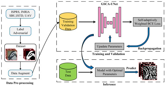
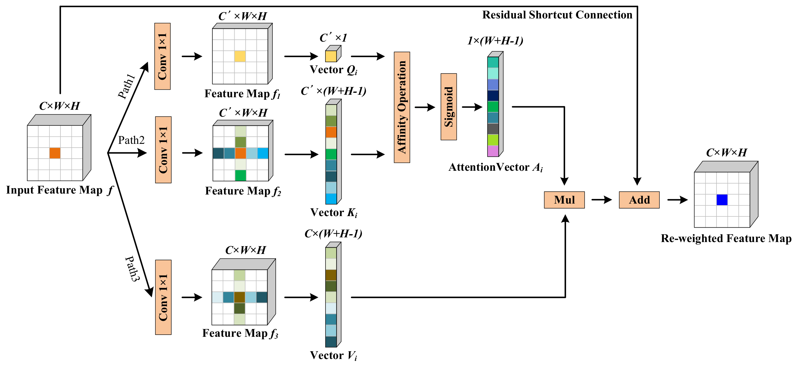
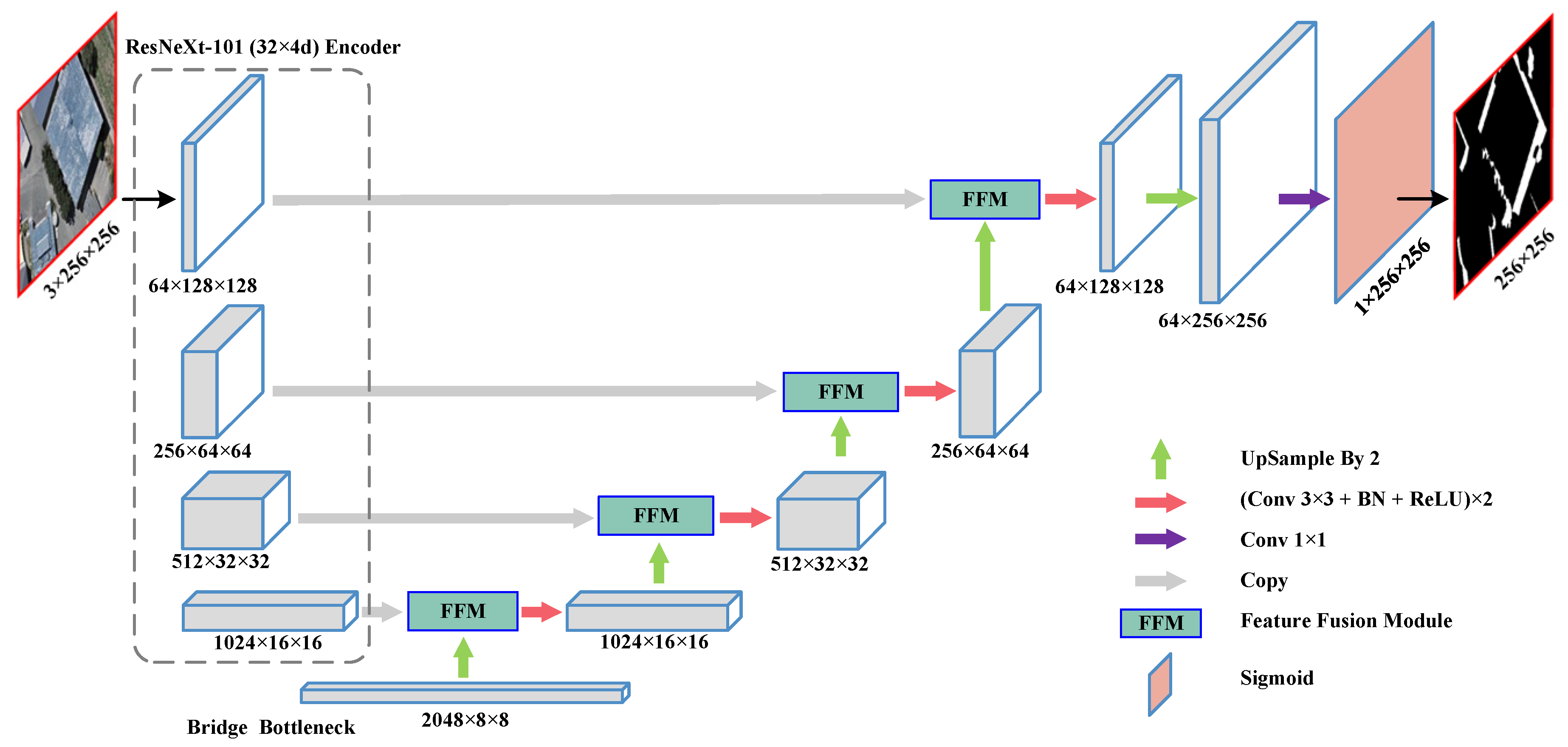
Inspired by the above analysis, in this paper we put forward a novel deep learning-based method, namely, a global-spatial-context attention U-shaped network (GSCA-UNet) to fill the gap between model automaticity and accuracy for shadow detection in urban aerial images. Experiment results on several typical urban aerial images verified the effectiveness and superiority of the proposed method. The main contributions of this work are listed as follows,
(1)
we developed a spatial-attention module to capture the long-ranged contextual information for each pixel, which contributed to identifying the challenging shadows and non-shadows;
(2)
on the basis of the UNet network architecture reported in [42], we realized end-to-end automatic and accurate shadow detection in urban aerial images; and
(3)
we developed a self-adaptively weighted binary cross-entropy (SAWBCE) loss function that enhanced the training procedure.
The remainder of this paper is organized as follows. Section 2 introduces the details of the proposed approach. Section 3 describes the experiment implementation and results. The method and experiments are discussed in Section 4. Last, this paper is concluded in Section 5.

2. Methodology

In this work, a CNN-based method is proposed for detecting shadows in urban aerial images. The overall flow of our method consists of the three following parts. First, a new shadow detection dataset including training and validation sets was constructed by labeling the selected sliced image tiles and adversarial preprocessing. Afterward, the proposed GSCA-UNet was trained on the dataset, and the optimal parameters were obtained under the supervision of the modified BCE loss function. Last, the chosen test images were fed into the well-trained model to produce the final shadow detection results. The intuitive pipeline of our method is given in Figure 1.

2.1. Data Preprocessing

As a data-driven method, the dataset is the key to deep learning-based methods. In previous studies, three benchmark shadow detection datasets (i.e., UCF, SBU [43], and ISTD [44]) were widely used. After many attempts, we found that the three datasets could not meet the needs of accurate shadow detection in urban aerial images. In addition to the model factor, the major reason was that images in these benchmarks could not model the complexity of shadows for urban aerial images because of the contained shadows that were mainly caused by individual trees, people, or cars. Therefore, a new dataset is urgently required to support shadow detection in urban aerial images. The three stages in our data preprocessing are as follows.
We first selected 17 images from the International Society for Photogrammetry and Remote Sensing (ISPRS) Urban Classification and 3D Building Reconstruction benchmark, the Inria Aerial Image Labeling dataset [45], and our own unmanned aerial vehicle (UAV) data captured by DJI Mavic2. All theses selected images have a very high spatial resolution and are characterized by quite a few heterogeneous shadows. Due to the limitation of the GPU device’s memory, we downsampled the chosen images, and sliced each image into small patches with a size of 256 × 256 pixels. After that, the boundaries of the shadow regions were manually depicted using A r c M a p 10.4 and L a b e l M e software; then, the raster labels were obtained. This process took about one month. We chose part of the patches to annotate instead of labeling each patch because there were many redundant patches with similar shadows or without shadows. We also selected 64 images from the SBU and ISTD benchmarks and added them into our dataset. By doing so, an initial dataset containing 2450 images was obtained.
A meager amount of data could easily make the deep learning model overfitted, while manually annotating a large dataset is labor-intensive and time-consuming. Facing this fact, the GAN principle was used in this work. Specifically, taking the major challenge of shadow detection into consideration, we employed data augmentation methods to generate two simple types of additional adversarial images to further enlarge the dataset. Unlike the work described in [39], the cumbersome training procedure was not required for our approach, reducing the complexity of the method. The first type of the adversarial image is shaded-variant images that were obtained by applying the gamma transformation. We only changed the intensity value of each pixel in the shaded regions, and the nonshaded regions remained unchanged. This transformation is described as
s = c r γ ,
where r denotes the original gray value of each shadow pixel, c and γ are two parameters to adjust the final result, and s is the transformed result. In this study, c = 1 and γ 0.6 , 0.7 , 0.8 , 1.2 , 1.4 , 1.6 . Given an input image, when γ < 1 , the shaded regions were brighter. Conversely, they were darker when γ > 1 . Like most image enhancement approaches [46], this transformation was performed on the V channel of the HSV color space. After transformation, six adversarial images with different color ranges in shades were obtained for every single image. As part of the shades might have been too bright after transformation, and this is unrealistic in real cases, the generated images with too-bright shaded regions were removed, as it might mislead the model to detecting false shadows. The second type of the adversarial images is disturbed-dark-object images. For this, we first selected images in which the non-shadow regions were larger. Subsequently, we randomly erased a polygonal region in the non-shadow region for each selected image. The size and shape were also random. To avoid that the erased region covered too large or too small a region, its size was limited to s [ 1 80 S n s , 1 20 S n s ] , where s and S n s denote the areas of erased and nonshaded regions, respectively. Last, the erased region was filled with a random dark color to model the challenging dark non-shadow objects. Figure 2 gives an example of the synthetic adversarial images obtained by using the proposed method.
Through the two procedures introduced above, 16,300 additional adversarial images were obtained. The generated adversarial images were added into the primary dataset, and the final dataset was constructed. Compared with the primary labeled dataset, the number of images was increased to 18,750 images, which enhanced the ability of the proposed GSCA-UNet model to characterize the unknown input shadows.

2.2. Global-Spatial-Context Attention Module

Researchers argued that the network that is capable of capturing more nonlocal contextual information plays a critical role in enhancing performance for semantic segmentation [47,48]. As shadow detection can be regarded as a dense pixel-level semantic-segmentation task, the global spatial semantic associations between pixels contained in an image are also crucial for accurate shadow detection, especially when there is no prior knowledge about the image scene.
To better demonstrate the necessity of the global spatial contextual information for shadow detection, three real instances are given in Figure 3. Figure 3a presents a typical case where the dark roof in non-shadowed regions is easily identified as a shadow. Figure 3b illustrates a case where a road with relatively high brightness in the shadow region is easily classified as non-shadow. The two given instances are widespread in urban aerial images. Applying the previous methods published in [19,20,22], we noted that only considering general shadow characteristics made it almost impossible to predict the true category for the two small images, as their local features (e.g., low brightness) are highly similar. However, if the two small images are both put back into the original image, this confusion is readily solved by comparing the distinction of brightness between the shaded regions where they are located with surrounding nonshaded regions. Taking Figure 3b as an example, the road in the shaded region could be determined as a shadow by comparing it with the adjacent nonshaded road because the former is relatively darker than the latter. Therefore, we needed to analyze the surrounding or larger regions to determine whether an object was a shadow or non-shadow. That is to say, to improve shadow detection performance requires to analyze the nonlocal relationships between pixels. The nonlocal relationships in this study were interpreted as the global spatial contextual information. The case in Figure 3c confirmed this analysis. When comparing C with the B, a strong indicator that C was a shadow was that B was brighter than C. However, comparing C with the A, A being darker than C would indicate that C was a non-shadow, even they were both shadows.
It is well known that the convolution operation, except for global convolution, only acts upon the adjacent pixels, and the long-ranged pixels are neglected. As a matter of fact, the informative correlation between pixels that are far from each other is also valuable. As analyzed above, if the shadow detection model could pay attention to larger (nonlocal) regions, it boosts performance of detection. Similar to the channel attention mechanism of SeNet [49], which weighs information on the channel dimension according to the importance of each channel, we designed an attention module to weigh each pixel in a different spatial position. Thus, the GSCA module was developed to clarify the importance of each pixel by aggregating the correlation between all pixels located in the same row and column.
The structure of the proposed GSCA module is shown in Figure 4. Given an input feature map f with a shape of C , W , H , where C, W, and H represent the number of channels, width, and height of feature map f, respectively, f is first fed to the 1 × 1 convolution layer in Paths 1 and 2 to compress the number of the channels, reducing computation cost, and generating two new feature maps f 1 and f 2 . The size of f 1 and f 2 is C , W , H , where C < C and C = 1 2 C in this study. Afterward, a feature vector Q i is extracted for the pixel with position i on the spatial dimension of feature map f 1 . At the same time, feature vector K i is obtained by extracting all pixels at the same row and column of the i-th pixel in feature map K. Dimensions of Q i and K i are C × 1 and C × H + W 1 , respectively. Inspired by DANet [50], the affinity operation (see Formula (2)) was applied to compute the degree of correlation between feature vectors Q i and K i . For the i-th pixel in f, the contextual information of all pixels in the same row and column where it is located is aggregated through the affinity operation. This procedure is only related to pixel location (spatial dimension).
d i , j = Q i T K i , j ,
where K i , j is the j-th element in the extracted feature vector K i from feature map f 2 ; i is the spatial pixel position; j = 1 , 2 , 3 , , W + H 1 , ⊗, vector multiplication; and d i , j is the computed degree of correlation between Q i and K i , j , with its dimension 1 × W + H 1 . d i , j was normalized using the sigmoid function to obtain attention vector A i , j . The sigmoid function is written as
S x = 1 1 + e x ,
where x, input tensor. In the attention vector A i , j , elements are suppressed or emphasized according to the corresponding feature responses, clarifying the contribution of each position, and pushing the model to consider more semantic regions. For Path 3 in the GSCA module, the 1 × 1 convolution layer was utilized to ensure that the model could learn nonlinear features between channels [51] and generate another feature vector V i with the shape of C × H + W 1 . V i collects all pixels in the same row and column from feature map f 3 . The global spatial contextual information is then aggregated by the element-wise summing result of A i , j and V i , j . In order to make the network quickly converge and reuse the features, residual identity mapping was added at the end of the GSCA module. The skip connection and identity mapping proved that it has significant positive impact on the convergence and accuracy of deep CNNs [52]. Therefore, the final reweighted feature map is obtained by
f i = j = 1 W + H 1 A i , j V i , j + f i , i = 1 , 2 , 3 , , W × H ,
where f i stands for the final reweighted feature map, and i denotes the spatial position of each pixel.
Applying the GSCA module over all pixels on the spatial dimension once, the global contextual information of each pixel in the horizontal and vertical directions was aggregated.

2.3. GSCA-UNet

2.3.1. Network Architecture

In this section, we present the details of the proposed GSCA-UNet. To date, due to the apparent advantage in the simple and effective symmetrical encoder–decoder structure, UNet has been widely applied for various remote-sensing tasks, such as building extraction [53], cloud detection [54], and urban village segmentation [55]. The UNet architecture can hierarchically aggregate low-level features from the shallow layer in the encoder path and high-level features from the decoder path by simple skip connection. Most importantly, UNet has proven to potentially be able to handle pixel-level semantic-segmentation tasks with a relatively small dataset. Because of these reasons, the U-shaped architecture was adopted as the baseline architecture in this study.
The original encoder path of UNet is constructed by stacking a sequence of basic blocks that consist of a 3 × 3 convolution layer, a batch-normalization (BN) layer, and a rectified-linear-unit (ReLU) layer. In order to achieve better performance, the ResNeXt-101 (32 × 4d) [56] network was adopted instead of the original UNet encoder to more effectively encode shadow features. ResNeXt-101 is the improved version of ResNet-101, which is the champion network in the Large-Scale Visual-Recognition Challenge (ILSVRC) competition in 2015. We removed the last three layers from the original ResNeXt-101 network, namely, the softmax, fully connected, and global average pooling layers. The final stage that outputs features with 2048 channels was served as the bridge bottleneck block, separating encoder from decoder. The other stages were utilized as the encoder backbone. As illustrated in Figure 5, the encoder path consists of four stages. Given an input image, when it passes through each stage of the encoder, the successive convolution and pooling-downsampling operations decrease the spatial dimension and increase the channel dimension. In order to output the predicted shadow maps that are the same size on the spatial dimension as the input image, a modified expansive path of UNet was adopted for this work. Unlike UNet, we utilized bilinear interpolation to replace the transposed convolution for performing the upsampling operation, which not only had minimal impact on the output of the model, but also effectively eliminated the checkerboard phenomenon resulting from transposed convolution. On the basis of the module that concatenates low-level and high-level features in UNet, the new feature fusion module (FFM) embedded two GSCA modules were developed. Through FFM, low-level and high-level features were first concatenated, and then the weighted feature map was obtained. The spatial size and the refined details were gradually restored by upsampling and 3 × 3 convolution operations. At the end of the decoder in GSCA-UNet, a 1 × 1 convolution layer was applied to compress the channel dimension from 64 to 1. Following that the nonlinearity sigmoid layer was applied to output the final shadow-prediction maps, where each pixel was encoded by the probability of belonging to shadow. The final binary shadow detection map was obtained by thresholding the prediction maps.

2.3.2. Feature Fusion Module

It is a gradual procedure to restore the size of a high-level feature map, requiring the fusion of low-level features to supply spatial-location information for improving the segmentation accuracy [57]. To meet the need for accurate shadow detection, we designed a new feature fusion module to fuse the high-level and low-level features, and weigh the fused feature maps. In FFM (see Figure 6), there are two inputs, namely, the low-level features from ResNeXt-101 encoder and the high-level features upsampled by earlier bilinear interpolation. The two inputs are first concatenated over channel dimension. Considering that the concatenated features usually have a high dimension, we applied a 1 × 1 convolution layer following it. The effect of 1 × 1 convolution in FFM can be interpreted as two aspects: compressing channels and nonlinear interaction between channels. The feature map f output by the 1 × 1 convolution layer was input to the first GSCA module to produce a temporary feature map f . Although the horizontal and vertical contextual information could be aggregated via a single GSCA module, the pixel-wise association between all pixels in f was still sparse, which was insufficient for accurate shadow detection. In order to obtain denser global spatial contextual information, another GSCA module was embedded. The two cascaded GSCA modules are called recurrent GSCA modules. f was again input into the second GSCA module to yield final reweighted features f . On the basis of the recurrent GSCA modules, each pixel in f contained dense pixel-wise global spatial contextual information. At the end of FFM, the final reweighted feature map f was input to the following convolution blocks for recovering details.

2.3.3. Modified Binary Cross-Entropy Loss

The loss function is a fundamental component in deep learning networks. During the backpropagation phase, the deviation between model predictions and ground truth is measured by loss function. Thus, loss function directly affects model performance. For two-class semantic-segmentation tasks, the BCE loss is a commonly used one, which is expressed as
l o s s p , y = y log p 1 y log 1 p ,
where p, prediction label; and y, ground-truth value.
For each training image, the shadow area proportion is not fixed. If the original BCE loss is directly utilized to supervise the training procedure, the imbalance of class distribution between shadows and non-shadows could affect the final detection accuracy. For instance, if we directly employed the original BCE loss, the model tended to detect relatively large non-shadows. To avoid the negative factor, we developed the SAWBCE loss. Unlike the weighted BCE loss in [58], the weight of the proposed loss function is self-adaptively acquired based on the prediction and ground truth at each iteration. The SAWBCE loss consists of two parts, i.e.,
l o s s 1 = N n N n + N s y log p N s N n + N s 1 y log 1 p
l o s s 2 = F N T P + F N y log p F P T N + F P 1 y log 1 p ,
where y, true label; and p, predicted label. In Equations (6) and (7), N n is the number of non-shadow pixels in the reference shadow map, N s is the number of shadow pixels in the reference shadow map, T P (true positive) is the total number of true shadow pixels that are correctly detected, and T N (true negative) is the number of true non-shadow pixels that are correctly detected. On the other hand, F P (false positive), number of non-shadow pixels that were mistakenly identified as shadow pixels; and F N (false negative), number of true shadow pixels that were detected as non-shadow pixels. The final SAWBCE loss is calculated by
l o s s = l o s s 1 + l o s s 2 ,
where l o s s 1 is applied to balance the area proportion of detected shadows and non-shadows, and l o s s 2 helps the model to focus on identifying difficult shadows [59]. Specifically, if the area of shadow regions in ground truth is smaller than that of non-shadow regions, l o s s 1 penalizes non-shadow regions more heavily than it does shadow regions. If a shadow area is larger than a non-shadow area, the shadow region receives a heavier penalty. If the correctly classified shadow regions are relatively small, l o s s 2 has a relatively larger value, and vice versa.

2.4. Training Details

The proposed GSCA-UNet shadow detection network was trained and evaluated on the constructed shadow dataset introduced in Section 2.1. The original dataset contained 18,750 images and corresponding binary labels. Before training, the hold-out strategy was adopted to split the dataset, and the divided ratio was set at 7:3. We randomly split 70% of the images for the training set to train the model, and 30% of images for the validation set to supervise whether the model was overfitted, and verify network performance during each training phase. The shadow image samples and corresponding annotated shadow labels of the training and validation sets are displayed in Figure 7.
In order to make the proposed GSCA-UNet model more robust, the following data augmentation methods were adopted for this research. For every single image in the training set, we first randomly flipped it horizontally and vertically. Then, we randomly rotated it with a degree of 90 , 90 , which aimed to handle the problem of shadow rotation. Last, we randomly resized it with scale 0.8 , 1 to deal with the shadow multiscale problem. The above probability values were all set to 0.8 in data augmentation.
For parameter initialization, the encoder and bridge block of GSCA-UNet were initialized by the parameters of the ResNeXt-101 network, which was pretrained well on the ImageNet dataset [60], and the other was initialized using Kaiming uniform [61]. We adopted the Adam [62] algorithm equipped with a weight decay rate of 0.0005 and an initial learning rate of 0.01 as the optimizer for the network. The exponential weight-decay strategy with a decay rate γ = 0.9 was employed to adjust the learning rate for each epoch. The number of epochs was set to 100 to make the network converge well. We set the minibatch size to 12 to make full use of the memory of GPU device in this study.

3. Experiments and Results

3.1. Test Images

Eight images cut out from several urban aerial images captured in different places were used as test images. All of these test images cover the dissimilar urban scenes and are characterized by quite a few shadows whose surfaces, shapes, and sizes are irregular. Among these test images, we selected four typical images (namely, the Toronto, Chicago, Vienna, and Austin images) for a better and fairer comparison between different state-of-the-art methods. The details of the four test images are displayed in Table 1. The Toronto and Chicago images were characterized by dense commercial buildings. For the two images, shadows were mainly attributed to the blocking from high-rise buildings, and the main obstacle for automatically detecting shadows is how to separate shadows from many misleading objects such as black vehicles, dark roofs, and nonuniform shadows with high brightness. In the Vienna image, there was a large number of shadows with a relatively small size caused by low-rise ridge-style buildings. The presence of many dark roofs and shadows with small sizes in this image made precisely detecting shadows greatly challenging. For the Austin image, the main urban land cover types are cement pavement and greenish water bodies that are often identified as shadows by traditional methods. Therefore, these test images were greatly suitable to verify the effectiveness of our approach.

3.2. Implementation Details

In the experiments, the proposed GSCA-UNet network was implemented on the basis of the PyTorch-1.1 framework in an Ubuntu 18.04 environment except for the GSCA module, which was done by CUDA programming using C++ programming language. All experiments were done on a workstation whose configurations are Intel Core i9-9900k CPU, 32 GB RAM, and an Nvidia GeForce RTX 2080ti GPU with 11 GB RAM.
The detailed variations of the loss value and overall accuracy at each training stage are displayed in Figure 8. Figure 8 shows that the convergence process of the proposed GSCA-UNet was stable, and overall accuracy exceeded 96%. Moreover, the overfitting phenomenon was not evident.

3.3. Comparison with State-Of-The-Art Methods

The performance of the proposed method was compared with three other reported state-of-the-art shadow detection methods for urban remote-sensing images, i.e., the image-matting method (IMM) [27], the extended-random-walker (ERW) method [20], and the object-oriented (OO) method [22]. The selection of the three methods was based on two considerations: (1) as an automatic shadow detection method, the proposed method had to compare with the same method type, and (2) because the supervised methods can usually deliver high accuracy with manual intervention, but most existing automatic detection methods exhibit relatively low accuracy, revealing the effectiveness of the proposed method requires making comparisons with the supervised methods with high accuracy. In addition, we compared our method with the bidirectional feature pyramid network (BFPN) with recurrent attention residual (RAR) modules. Note, the method is called BDRAR for short in the following section. BDRAR is CNN-based and achieved nearly saturated performance of 3.64 and 5.30 on the SBU and UCF datasets, respectively, for balanced error rate [40].
From these methods, we implemented the IMM and the OO method using the default parameters given in the corresponding literature. Before implementing the IMM, we marked abundant scribes using P h o t o s h o p software. In the ERW method, because the scenes of the test images being extremely complex, they always achieved poor performance for all test images. Therefore, we fine-tuned the threshold level to obtain the best results according to the specific image. We trained the BDRAR model with the best performance on our dataset using the training strategies given by the authors.

3.3.1. Visualization Results

The visualization results of the final shadow detection of our approach and of the four state-of-the-art methods are presented in Figure 9, Figure 10, Figure 11 and Figure 12, from which we can observe that these methods were capable of extracting most shadows in diverse cases.
The obtained results by the IMM method look reasonable compared to the reference shadow maps. However, as shown in Figure 9c, Figure 10c, Figure 11c, Figure 12c, quite a few positive (shadow) and negative (non-shadow) samples were needed to be labeled in advance to yield the final detection results for each input image. Another obvious weakness of the IMM method can be found from Figure 9c and Figure 10c, where some small shadows were missed, which was caused by the fact that it is arduous to mark small shadows. In addition, the image-matting procedure for the IMM method occupied too much computer memory, and the computation speed was very slow when the size of an input image that contained a great many shadows was large. As a result, the IMM method had lower automaticity, which limits the practical applications.
The OO method maintained well the integrity of the detected shadow regions. As illustrated in Figure 9e, Figure 10e, Figure 11e, Figure 12e, applying the object- instead of the pixel-based strategy effectively eliminated the adverse phenomenon in detected shadow maps, such as fragmented shadows and holes. Meanwhile, compared to the ERW method, this method reduced the interference to some extent from dark objects. For example, part of the black vehicles was correctly ruled out in the Toronto and Chicago images. Unfortunately, the OO method failed to handle the nonuniform shadows in the Toronto image and the dark water body in the Austin image. In Figure 9e, this method classified vehicles with bright surfaces in shaded regions as non-shadows. In Figure 12e, because the river had similar low-intensity features to those of shadows, it was detected as shadows. Another disadvantage of the OO method is that it is hard to obtain optimal segmentation parameters with it. Although the state-of-the-art multiscale segmentation method [63,64,65] was adopted in the experiments, the oversegmentation phenomenon still occurred. Taking the Austin image as an example, the OO method failed to separate trees and correspondingly casted shadows, which affected detection accuracy.
Benefiting from the great advantage in feature extraction and the employed recurrent residual attention module, the BDRAR method produced satisfactory detection results. However, it can be seen in Figure 12 that it was insufficient to precisely locate the shadow boundaries, and part of the shadows was missed due to lack of consideration for global spatial contextual information. In terms of identifying dark objects, there were many wrongly labeled shadows in the Toronto and Vienna images, leading to poor performance.
On the foundation of the U-shape-based fully convolutional neural network and the global-spatial-context attention module, compared with the other methods, our method always obtained remarkable shadow detection results that were the most consistent with the reference shadow maps. A striking illustration of the results obtained by our method is shown in Figure 9g, Figure 10g, Figure 11g, Figure 12g, from which we can see that there was little noise, and most of the shadows and non-shadows were precisely detected. When handling the four input images that contained many dark non-shadows and bright shadows, the performance of the other automatic methods was insufficient. In contrast, our method effectively suppressed these negative effects due to fully exploiting the global spatial contextual information of each pixel. Taking two difficult cases in the Toronto image as an example, as illustrated in Figure 13, the black car marked with blue was identified as shadows by all compared methods as the contextual information of long-ranged pixels was ignored, while our method detected it correctly by considering the global spatial contextual information. On the other hand, the proposed GSCA-UNet also completely detected the other challenging bright and nonuniform shadow regions marked with red by comprehensively analyzing the near regions. The close-up results shown in Figure 13 confirmed that global spatial contextual information plays a positive effect on shadow detection. Most importantly, our method was able to produce accurate shadow detection results in diverse images with different light conditions, projected surfaces, and occlusions, without any user intervention or prior knowledge.
From the aforementioned comparisons, we could conclude that the balance between automaticity and accuracy for the proposed method was better than that of other advanced methods.

3.3.2. Quantitative Comparisons

To further objectively evaluate the performance of different methods, following the works in [8,18,20], two popular evaluation metrics for the pixel-level classification task, i.e., F1-score ( F 1 ) and overall accuracy ( O A ), were adopted to quantitatively validate detection performance in the subsequent accuracy assessment. We also employed the balanced error rate ( B E R ) [32,37,38,39,43] that is widely used for shadow detection in natural images. As shadow detection can be regarded as a semantic-segmentation task, we also utilized intersection over union ( I o U ) as a commonly used metric for semantic-segmentation tasks to validate the proposed network. The four metrics are expressed as
P r e c i s i o n = T P T P + F P × 100 % , R e c a l l = T P T P + F N × 100 %
F 1 = 2 × P r e c i s i o n × R e c a l l P r e c i s i o n + R e c a l l × 100 %
O A = T P + T N T P + T N + F N + F P × 100 %
B E R = 1 1 2 T P T P + F N + T N T N + F P × 100 %
I o U = T P T P + F P + F N × 100 %
In Equations (9)–(13), T P (true positive) is the total number of true shadow pixels that were correctly detected, T N (true negative) is the number of true non-shadow pixels that were correctly detected, F P (false positive) is the number of the non-shadow pixels that were mistakenly identified as shadow pixels, and F N (false negative) is the number of true shadow pixels that were detected as non-shadow pixels.
In our two-class pixel-level shadow and non-shadow classification task, F 1 reports the numerical assessment of the method by taking both precision and recall into consideration, with a higher value meaning that model performance was better; O A assesses the rate in which pixels are correctly detected as part of their true categories; B E R indicates the balanced error rate for shadow and non-shadow error rates; I o U measures the intersection ratio between actually detected shadows and true shadows. Comparing the results of the IMM, ERW, OO, BDRAR methods and ours, Table 2 and Table 3 clearly show that our method had the best values in terms of F 1 , O A , B E R , and I o U . From the Toronto to the Austin images, with the increase in difficulty for shadow detection, the performance of all methods was more or less reduced. For the two conventional automatic methods (ERW and OO) and the CNN-based BDRAR method, a sharp reduction in performance was observed in the Vienna and Austin images, especially Austin, which was mainly covered by dark water. The ERW and OO methods reached very low I o U values (29.11% and 28.97%), while our method’s I o U value was 77.18%. Even if compared to the supervised IMM method, the I o U value (77.18%) of our method was still higher than that of the IMM (63.07%). From the quantitative comparisons, it can be concluded that our approach could acquire high-accuracy results while maintaining automaticity, which again powerfully demonstrates the effectiveness and superiority of the proposed method for shadow detection in urban aerial images.

4. Discussion

4.1. Network-Design Evaluation

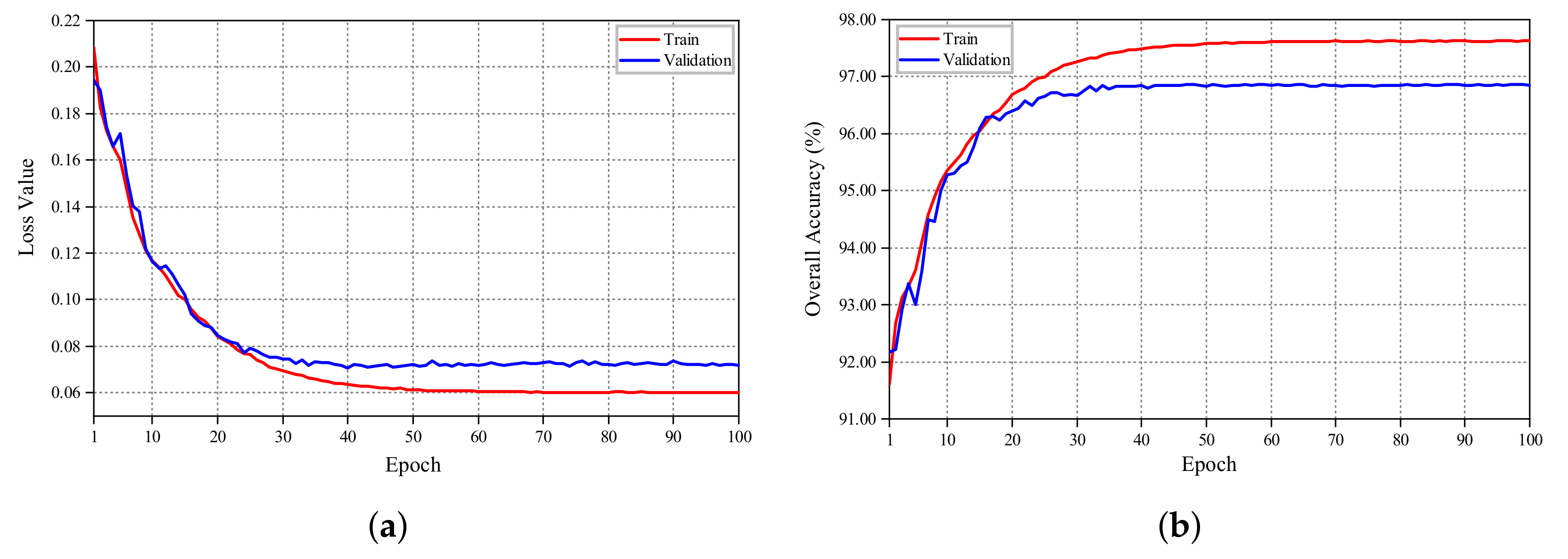
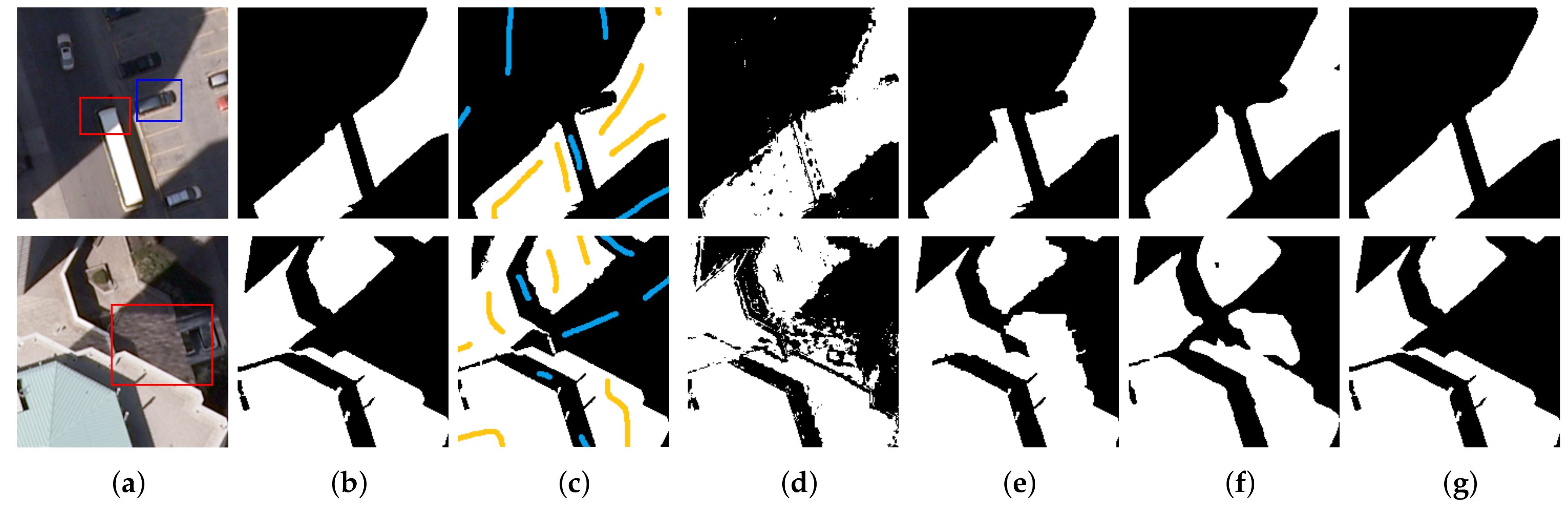
In this section, we evaluate the network design of the proposed GSCA-UNet. To better test and verify the effects of different network structures for shadow detection, we performed comparative experiments with the two other CNNs. The first network was the original UNet without the GSCA module and the ResNeXt-based encoder part, and the second was ResNeXt101-UNet, which was derived by removing the GSCA module from GSCA-UNet. Compared with our network, the complexity of the network structure of the two models above increased, and similarity with our model was high. Accordingly, the two models were suitable to verify the feature extractor of ResNeXt-101 and the GSCA module, respectively. We trained UNet and ResNeXt-UNet on our dataset by using the same loss function and training strategy to ensure analysis credibility. Detailed comparison results are displayed in Table 4. As illustrated in Table 4, compared with the baseline UNet network, utilizing the ResNeXt-101 as feature encoder improved F 1 , O A , B E R , and I o U by 0.58%, 0.22%, 6.48%, and 1.03%. The main reason for the improvement is that, compared with the original encoder part, the ResNeXt-101 network not only had the advantage of a residual shortcut, but also had a deeper and wider structure, enhancing its ability to extract shadow features. After embedding the recurrent GSCA module, Table 4 shows that F 1 , O A , B E R , and I o U were significantly improved by 4.47%, 1.72%, 31.3%, and 7.77%, respectively, which validated the effectiveness of the GSCA module. The reason why the proposed GSCA module could obviously improve performance could be that we established the global link between pixels by enlarging the receptive filed of the CNN by using the module. Although the receptive filed of a CNN model can be theoretically increased by stacking many convolution layers, or applying the atrous convolution operations [66] or the spatial-pyramid-pooling (SPP) module [67,68], the structural limitation of the convolution kernel makes the model only learn the local dependence for each pixel in each stage even if the network contains deeper layers. Therefore, for each pixel, the global spatial contextual information in the feature maps obtained by the ResNeXt101-UNet network was absent. Applying the GSCA module twice in each feature-fusion module, the concatenated feature map paid attention to global contextual information, and each pixel in the spatial dimension was reweighed. The dense global spatial contextual information for each pixel contributed to better identifying suspected shadows. Therefore, the model could more precisely locate shadows. To test the importance of the SAWBCE loss function, we conducted comparison experiments with the original BCE loss and SAWBCE loss. We used two GSCA-UNet models that were trained with BCE and SAWBCE loss, respectively. As listed in Table 5, the proposed model with SAWBCE loss had the best shadow detection accuracy.

4.2. Advantages of the Proposed Method

Shadow detection in urban aerial images has been a popular research topic in the last few decades, yet automatic and accurate methods to detect shadows are still lacking. The proposed method in this paper filled this gap. Benefiting from dense global spatial contextual information, our method could yield accurate results without any manual intervention or prior knowledge in diverse cases, even compared with the representative supervised IMM method, which can usually obtain results with high accuracy. The proposed method is based on deep learning technology. Under the support of sufficient image data, it can be transferred to other unknown shadow detection tasks. For practical applications, the precisely detected shadows by our proposed method are more suitable as useful information for corresponding studies, such as urban-building instance recognition, building height estimation, and information recovery. At the same time, the proposed GSCA module has the advantage of flexibility. It can be applied to other CNN-based dense semantic-segmentation tasks for urban aerial remote sensing images, such as building extraction.

4.3. Limitations and Further Improvements

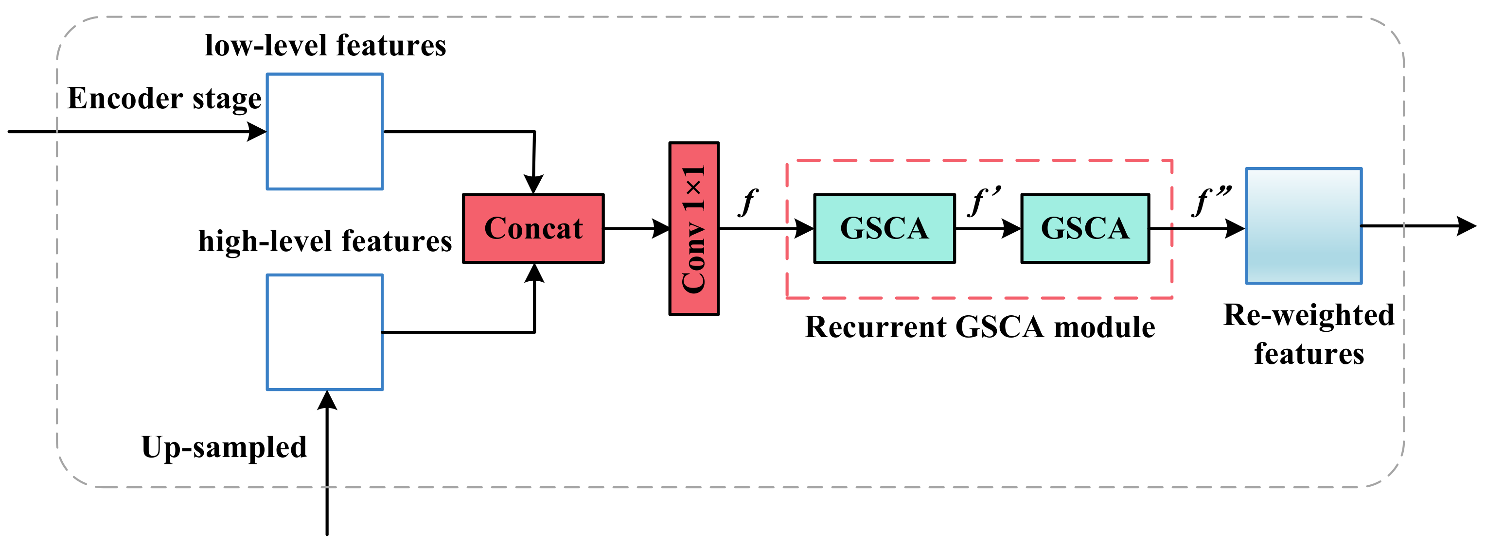
Although the proposed shadow detection method filled the gap left by the inadequate balance between automaticity and accuracy, some inherent weaknesses should not be ignored. Generally, spatial information in low-level features helps to locate shadow regions, but low-level features might bring unexpected noise that could cause detection errors. In this study, we directly concatenated the low- and high-level features via skip connection, and the spatial information of the shallow layer and contextual information were not leveraged. Thus, an individual feature fusion module is suggested to rethink the relationship between low- and corresponding high-level features in the feature fusion model.
To aggregate spatial contextual information in the horizontal and vertical directions requires to perform the iterative process pixel by pixel, which comes with high computation cost. The time complexity is O W × H × W + H 1 on the channel dimension when the size of the input tensor is ( B , C , W , H ), where B, C, W, and H are batch size, channel number, width, and height, receptively. In this study, with size (12, 3, 256, 256) of the initial input, it took about 75.40 min to train each epoch, and 0.11 s to inference, which was relatively slow. On the other hand, the number of parameters for the proposed GSCA-UNet was 106.04 million, making the GSCA-UNet impractical for implementation on some lightweight platforms. Future work should pay more attention to decreasing the number of network parameters to achieve real-time detection.

5. Conclusions

Although tremendous efforts have been devoted to coping with the challenge of automatic and accurate shadow detection in urban aerial images over many years, it still remains a challenging problem due to the limitation of feature patterns and not considering nonlocal contextual information. In this paper, a new end-to-end deep-learning-based shadow detection method was proposed to address this issue. On the basis of the popular U-shaped architecture of the UNet network, the developed GSCA modules were embedded to self-adaptively aggregate global contextual information for each pixel and generate weighted feature maps. Experiments performed on several typical urban aerial images demonstrated that the proposed shadow detection method could effectively suppress the negative effects such as salt-and-pepper noise, holes, and inaccurate boundary locations of the detected shadow regions. Compared with four state-of-art supervised and unsupervised methods in terms of visual interpretation and several quantitative evaluation metrics, our method exhibited the best performance without any human intervention and prior knowledge, which revealed the superiority of the proposed method in maintaining a balance between automaticity and accuracy. There still remain some issues, such as costly computation and the large number of network parameters. In the future, a larger dataset should be supplemented, and a lightweight network should be developed to achieve real-time detection.

Author Contributions

Y.J. overall conceived and designed the experiments; W.X. acquired funding and supervised the entire experiment; Y.J. performed the experiments; Y.J. wrote the manuscript; Z.H. reviewed and revised the manuscript; D.S. and H.J. collected and annotated data; and X.L. annotated the data. All authors have read and agreed to the published version of the manuscript.

Funding

This research was funded by Sichuan Province Science and Technology Support Programs nos. 2018GZDZX0034, 2018GZDZX00, 2019YFG0382, and 2019YFG0202).

Acknowledgments

The authors thank the ISPRS and Inria for providing the open access and free aerial image dataset for constructing the shadow detection dataset. The authors are also grateful to H. Li and X. Kang for providing the codes for their methods. The authors would also like to thank anonymous reviewers and the editor for their insightful comments and helpful suggestions.

Conflicts of Interest

The authors declare no conflict of interest.

Abbreviations

The following abbreviations are used in this manuscript.
UAVUnmanned aerial vehicle
GPUGraphics processing unit
HSVHue-saturation-value
CUDACompute unified device architecture

References

  1. Azevedo, S.; Silva, E.; Pedrosa, M. Shadow detection improvement using spectral indices and morphological operators in urban areas in high resolution images. Int. Arch. Photogramm. Remote Sens. Spat. Inf. Sci. ISPRS Arch. 2015, W3, 587–592. [Google Scholar] [CrossRef] [Green Version]
  2. Wu, W.; Li, Q.; Zhang, Y.; Du, X.; Wang, H. Two-Step Urban Water Index (TSUWI): A New Technique for High-Resolution Mapping of Urban Surface Water. Remote Sens. 2018, 10, 1704. [Google Scholar] [CrossRef] [Green Version]
  3. Xie, C.; Huang, X.; Zeng, W.; Fang, X. A novel water index for urban high-resolution eight-band WorldView-2 imagery. Int. J. Digit. Earth 2016, 9, 925–941. [Google Scholar] [CrossRef]
  4. Ok, A.O. Automated detection of buildings from single VHR multispectral images using shadow information and graph cuts. ISPRS J. Photogramm. Remote Sens. 2013, 86, 21–40. [Google Scholar] [CrossRef]
  5. Huang, X.; Zhang, L. Morphological building/shadow index for building extraction from high-resolution imagery over urban areas. IEEE J. Sel. Top. Appl. Earth Obs. Remote Sens. 2011, 5, 161–172. [Google Scholar] [CrossRef]
  6. Liasis, G.; Stavrou, S. Satellite images analysis for shadow detection and building height estimation. ISPRS J. Photogramm. Remote Sens. 2016, 119, 437–450. [Google Scholar] [CrossRef]
  7. Adeline, K.; Chen, M.; Briottet, X.; Pang, S.; Paparoditis, N. Shadow detection in very high spatial resolution aerial images: A comparative study. ISPRS J. Photogramm. Remote Sens. 2013, 80, 21–38. [Google Scholar] [CrossRef]
  8. Cameron, M.; Kumar, L. Diffuse Skylight as a Surrogate for Shadow Detection in High-Resolution Imagery Acquired Under Clear Sky Conditions. Remote Sens. 2018, 10, 1185. [Google Scholar] [CrossRef] [Green Version]
  9. Xue, L.; Yang, S.; Li, Y.; Ma, J. An automatic shadow detection method for high-resolution remote sensing imagery based on polynomial fitting. Int. J. Remote Sens. 2019, 40, 2986–3007. [Google Scholar] [CrossRef]
  10. Zhou, K.; Lindenbergh, R.; Gorte, B. Automatic Shadow Detection in Urban Very-High-Resolution Images Using Existing 3D Models for Free Training. Remote Sens. 2019, 11, 72. [Google Scholar] [CrossRef] [Green Version]
  11. Tsai, V.J. A comparative study on shadow compensation of color aerial images in invariant color models. IEEE Trans. Geosci. Remote Sens. 2006, 44, 1661–1671. [Google Scholar] [CrossRef]
  12. Su, N.; Zhang, Y.; Tian, S.; Yan, Y.; Miao, X. Shadow detection and removal for occluded object information recovery in urban high-resolution panchromatic satellite images. IEEE J. Sel. Top. Appl. Earth Obs. Remote Sens. 2016, 9, 2568–2582. [Google Scholar] [CrossRef]
  13. Song, H.; Huang, B.; Zhang, K. Shadow detection and reconstruction in high-resolution satellite images via morphological filtering and example-based learning. IEEE Trans. Geosci. Remote Sens. 2013, 52, 2545–2554. [Google Scholar] [CrossRef]
  14. Chung, K.L.; Lin, Y.R.; Huang, Y.H. Efficient shadow detection of color aerial images based on successive thresholding scheme. IEEE Trans. Geosci. Remote Sens. 2008, 47, 671–682. [Google Scholar] [CrossRef]
  15. Silva, G.F.; Carneiro, G.B.; Doth, R.; Amaral, L.A.; de Azevedo, D.F. Near real-time shadow detection and removal in aerial motion imagery application. ISPRS J. Photogramm. Remote Sens. 2018, 140, 104–121. [Google Scholar] [CrossRef]
  16. Besheer, M.; Abdelhafiz, A. Modified invariant colour model for shadow detection. Int. J. Remote Sens. 2015, 36, 6214–6223. [Google Scholar] [CrossRef]
  17. Huang, W.; Bu, M. Detecting shadows in high-resolution remote-sensing images of urban areas using spectral and spatial features. Int. J. Remote Sens. 2015, 36, 6224–6244. [Google Scholar] [CrossRef]
  18. Mostafa, Y.; Abdelhafiz, A. Accurate shadow detection from high-resolution satellite images. IEEE Geosci. Remote Sens. Lett. 2017, 14, 494–498. [Google Scholar] [CrossRef]
  19. Ma, H.; Qin, Q.; Shen, X. Shadow segmentation and compensation in high resolution satellite images. In Proceedings of the 2008 IEEE International Geoscience and Remote Sensing Symposium (IGARSS), Boston, MA, USA, 7–11 July 2008; Volume 2, pp. II-1036–II-1039. [Google Scholar]
  20. Kang, X.; Huang, Y.; Li, S.; Lin, H.; Benediktsson, J.A. Extended random walker for shadow detection in very high resolution remote sensing images. IEEE Trans. Geosci. Remote Sens. 2017, 56, 867–876. [Google Scholar] [CrossRef]
  21. Zhang, H.; Sun, K.; Li, W. Object-oriented shadow detection and removal from urban high-resolution remote sensing images. IEEE Trans. Geosci. Remote Sens. 2014, 52, 6972–6982. [Google Scholar] [CrossRef]
  22. Mo, N.; Zhu, R.; Yan, L.; Zhao, Z. Deshadowing of urban airborne imagery based on object-oriented automatic shadow detection and regional matching compensation. IEEE J. Sel. Top. Appl. Earth Obs. Remote Sens. 2018, 11, 585–605. [Google Scholar] [CrossRef]
  23. Wang, Q.; Yan, L.; Yuan, Q.; Ma, Z. An automatic shadow detection method for VHR remote sensing orthoimagery. Remote Sens. 2017, 9, 469. [Google Scholar] [CrossRef] [Green Version]
  24. Tolt, G.; Shimoni, M.; Ahlberg, J. A shadow detection method for remote sensing images using VHR hyperspectral and LIDAR data. In Proceedings of the 2011 IEEE International Geoscience and Remote Sensing Symposium (IGARSS), Vancouver, BC, Canada, 24–29 July 2011; pp. 4423–4426. [Google Scholar]
  25. Richter, R.; Müller, A. De-shadowing of satellite/airborne imagery. Int. J. Remote Sens. 2005, 26, 3137–3148. [Google Scholar] [CrossRef]
  26. Yamazaki, F.; Liu, W.; Takasaki, M. Characteristics of shadow and removal of its effects for remote sensing imagery. In Proceedings of the 2009 IEEE International Geoscience and Remote Sensing Symposium, Cape Town, South Africa, 12–17 July 2009; Volume 4, pp. IV-426–IV-429. [Google Scholar]
  27. Li, H.; Zhang, L.; Shen, H. An adaptive nonlocal regularized shadow removal method for aerial remote sensing images. IEEE Trans. Geosci. Remote Sens. 2013, 52, 106–120. [Google Scholar] [CrossRef]
  28. Levin, A.; Lischinski, D.; Weiss, Y. A closed-form solution to natural image matting. IEEE Trans. Pattern Anal. Mach. Intell. 2007, 30, 228–242. [Google Scholar] [CrossRef] [Green Version]
  29. Liu, J.; Fang, T.; Li, D. Shadow detection in remotely sensed images based on self-adaptive feature selection. IEEE Trans. Geosci. Remote Sens. 2011, 49, 5092–5103. [Google Scholar]
  30. Lorenzi, L.; Melgani, F.; Mercier, G. A complete processing chain for shadow detection and reconstruction in VHR images. IEEE Trans. Geosci. Remote Sens. 2012, 50, 3440–3452. [Google Scholar] [CrossRef]
  31. Vicente, T.F.Y.; Hoai, M.; Samaras, D. Leave-one-out kernel optimization for shadow detection and removal. IEEE Trans. Pattern Anal. Mach. Intell. 2017, 40, 682–695. [Google Scholar] [CrossRef]
  32. Guo, R.; Dai, Q.; Hoiem, D. Paired regions for shadow detection and removal. IEEE Trans. Pattern Anal. Mach. Intell. 2012, 35, 2956–2967. [Google Scholar] [CrossRef]
  33. Ren, S.; He, K.; Girshick, R.; Sun, J. Faster R-CNN: Towards Real-Time Object Detection with Region Proposal Networks. IEEE Trans. Pattern Anal. Mach. Intell. 2017, 39, 1137–1149. [Google Scholar] [CrossRef] [Green Version]
  34. He, K.; Gkioxari, G.; Dollár, P.; Girshick, R. Mask r-cnn. In Proceedings of the IEEE International Conference on Computer Vision, Venice, Italy, 22–29 October 2017; pp. 2961–2969. [Google Scholar]
  35. Krizhevsky, A.; Sutskever, I.; Hinton, G.E. Imagenet classification with deep convolutional neural networks. In Proceedings of the Advances in Neural Information Processing Systems, Lake Tahoe, Spain, 3–6 December 2012; pp. 1097–1105. [Google Scholar]
  36. Khan, S.H.; Bennamoun, M.; Sohel, F.; Togneri, R. Automatic feature learning for robust shadow detection. In Proceedings of the 2014 IEEE Conference on Computer Vision and Pattern Recognition, Columbus, OH, USA, 23–28 June 2014; pp. 1939–1946. [Google Scholar]
  37. Hosseinzadeh, S.; Shakeri, M.; Zhang, H. Fast shadow detection from a single image using a patched convolutional neural network. In Proceedings of the 2018 IEEE/RSJ International Conference on Intelligent Robots and Systems (IROS), Madrid, Spain, 1–5 October 2018; pp. 3124–3129. [Google Scholar]
  38. Nguyen, V.; Yago Vicente, T.F.; Zhao, M.; Hoai, M.; Samaras, D. Shadow detection with conditional generative adversarial networks. In Proceedings of the IEEE International Conference on Computer Vision, Venice, Italy, 22–29 October 2017; pp. 4510–4518. [Google Scholar]
  39. Le, H.; Vicente, T.F.Y.; Nguyen, V.; Hoai, M.; Samaras, D. A+ D-Net: Shadow detection with adversarial shadow attenuation. Lect. Notes Comput. Sci. 2018, 11206, 680–696. [Google Scholar]
  40. Zhu, L.; Deng, Z.; Hu, X.; Fu, C.W.; Xu, X.; Qin, J.; Heng, P.A. Bidirectional feature pyramid network with recurrent attention residual modules for shadow detection. In Proceedings of the European Conference on Computer Vision (ECCV), Munich, Germany, 8–14 September 2018; pp. 121–136. [Google Scholar]
  41. Ding, B.; Long, C.; Zhang, L.; Xiao, C. Argan: Attentive recurrent generative adversarial network for shadow detection and removal. In Proceedings of the IEEE International Conference on Computer Vision, Seoul, Korea, 27 October–2 November 2019; pp. 10213–10222. [Google Scholar]
  42. Ronneberger, O.; Fischer, P.; Brox, T. U-net: Convolutional networks for biomedical image segmentation. In Proceedings of the International Conference on Medical Image Computing and Computer-Assisted Intervention, Munich, Germany, 5–9 October 2015; Springer: Berlin/Heidelberg, Germany, 2015; pp. 234–241. [Google Scholar]
  43. Vicente, T.F.Y.; Hou, L.; Yu, C.P.; Hoai, M.; Samaras, D. Large-scale training of shadow detectors with noisily-annotated shadow examples. In Proceedings of the European Conference on Computer Vision, Amsterdam, The Netherlands, 8–16 October 2016; Springer: Berlin/Heidelberg, Germany, 2016; pp. 816–832. [Google Scholar]
  44. Wang, J.; Li, X.; Yang, J. Stacked conditional generative adversarial networks for jointly learning shadow detection and shadow removal. In Proceedings of the IEEE Conference on Computer Vision and Pattern Recognition, Salt Lake City, UT, USA, 18–23 June 2018; pp. 1788–1797. [Google Scholar]
  45. Maggiori, E.; Tarabalka, Y.; Charpiat, G.; Alliez, P. Can Semantic Labeling Methods Generalize to Any City? The Inria Aerial Image Labeling Benchmark. In Proceedings of the IEEE International Geoscience and Remote Sensing Symposium (IGARSS), Fort Worth, TX, USA, 23–28 July 2017. [Google Scholar]
  46. Cheng, M.H.; Huang, T.Z.; Zhao, X.L.; Ma, T.H.; Huang, J. A variational model with hybrid Hyper-Laplacian priors for Retinex. Appl. Math. Model. 2019, 66, 305–321. [Google Scholar] [CrossRef]
  47. Yu, C.; Wang, J.; Peng, C.; Gao, C.; Yu, G.; Sang, N. Bisenet: Bilateral segmentation network for real-time semantic segmentation. In Proceedings of the European Conference on Computer Vision (ECCV), Munich, Germany, 8–14 September 2018; pp. 325–341. [Google Scholar]
  48. Yuan, Y.; Wang, J. Ocnet: Object context network for scene parsing. arXiv 2018, arXiv:1809.00916. [Google Scholar]
  49. Hu, J.; Shen, L.; Sun, G. Squeeze-and-Excitation Networks. In Proceedings of the IEEE Conference on Computer Vision and Pattern Recognition (CVPR), Salt Lake City, UT, USA, 18–23 June 2018. [Google Scholar]
  50. Fu, J.; Liu, J.; Tian, H.; Li, Y.; Bao, Y.; Fang, Z.; Lu, H. Dual attention network for scene segmentation. In Proceedings of the IEEE Conference on Computer Vision and Pattern Recognition, Long Beach, CA, USA, 15–21 June 2019; pp. 3146–3154. [Google Scholar]
  51. Szegedy, C.; Liu, W.; Jia, Y.; Sermanet, P.; Reed, S.; Anguelov, D.; Erhan, D.; Vanhoucke, V.; Rabinovich, A. Going deeper with convolutions. In Proceedings of the IEEE Conference on Computer Vision and Pattern Recognition, Boston, MA, USA, 7–12 June 2015; pp. 1–9. [Google Scholar]
  52. He, K.; Zhang, X.; Ren, S.; Sun, J. Deep residual learning for image recognition. In Proceedings of the IEEE Conference on Computer Vision and Pattern Recognition, Las Vegas, NV, USA, 27–30 June 2016; pp. 770–778. [Google Scholar]
  53. Wagner, F.H.; Dalagnol, R.; Tarabalka, Y.; Segantine, T.Y.; Thomé, R.; Hirye, M. U-Net-Id, an Instance Segmentation Model for Building Extraction from Satellite Images—Case Study in the Joanópolis City, Brazil. Remote Sens. 2020, 12, 1544. [Google Scholar] [CrossRef]
  54. Jiao, L.; Huo, L.; Hu, C.; Tang, P. Refined UNet: UNet-Based Refinement Network for Cloud and Shadow Precise Segmentation. Remote Sens. 2020, 12, 2001. [Google Scholar] [CrossRef]
  55. Pan, Z.; Xu, J.; Guo, Y.; Hu, Y.; Wang, G. Deep Learning Segmentation and Classification for Urban Village Using a Worldview Satellite Image Based on U-Net. Remote Sens. 2020, 12, 1574. [Google Scholar] [CrossRef]
  56. Xie, S.; Girshick, R.; Dollár, P.; Tu, Z.; He, K. Aggregated residual transformations for deep neural networks. In Proceedings of the IEEE Conference on Computer Vision and Pattern Recognition, Honolulu, HI, USA, 21–26 July 2017; pp. 1492–1500. [Google Scholar]
  57. Chen, L.C.; Zhu, Y.; Papandreou, G.; Schroff, F.; Adam, H. Encoder-decoder with atrous separable convolution for semantic image segmentation. In Proceedings of the European conference on computer vision (ECCV), Munich, Germany, 8–14 September 2018; pp. 801–818. [Google Scholar]
  58. Wang, Y.; Chen, C.; Ding, M.; Li, J. Real-time dense semantic labeling with dual-Path framework for high-resolution remote sensing image. Remote Sens. 2019, 11, 3020. [Google Scholar] [CrossRef] [Green Version]
  59. Shrivastava, A.; Gupta, A.; Girshick, R. Training region-based object detectors with online hard example mining. In Proceedings of the IEEE Conference on Computer Vision and Pattern Recognition, Las Vegas, NV, USA, 27–30 June 2016; pp. 761–769. [Google Scholar]
  60. Deng, J.; Dong, W.; Socher, R.; Li, L.J.; Li, K.; Fei-Fei, L. Imagenet: A large-scale hierarchical image database. In Proceedings of the 2009 IEEE Conference on Computer Vision and Pattern Recognition, Miami, FL, USA, 20–25 June 2009; pp. 248–255. [Google Scholar]
  61. He, K.; Zhang, X.; Ren, S.; Sun, J. Delving deep into rectifiers: Surpassing human-level performance on imagenet classification. In Proceedings of the IEEE International Conference on Computer Vision, Las Condes, Chile, 11–18 December 2015; pp. 1026–1034. [Google Scholar]
  62. Da, K. A method for stochastic optimization. arXiv 2014, arXiv:1412.6980. [Google Scholar]
  63. Baatz, M.; Schäpe, A. Multiresolution Segmentation: An Optimization Approach for High Quality Multi-Scale Image Segmentation. 2010. Available online: http://www.agit.at/papers/2000/baatz_FP_12.pdf (accessed on 20 December 2019).
  64. Hu, Z.; Li, Q.; Zou, Q.; Zhang, Q.; Wu, G. A bilevel scale-sets model for hierarchical representation of large remote sensing images. IEEE Trans. Geosci. Remote Sens. 2016, 54, 7366–7377. [Google Scholar] [CrossRef]
  65. Hu, Z.; Zhang, Q.; Zou, Q.; Li, Q.; Wu, G. Stepwise evolution analysis of the region-merging segmentation for scale parameterization. IEEE J. Sel. Top. Appl. Earth Obs. Remote Sens. 2018, 11, 2461–2472. [Google Scholar] [CrossRef]
  66. Chen, L.C.; Papandreou, G.; Kokkinos, I.; Murphy, K.; Yuille, A.L. Semantic image segmentation with deep convolutional nets and fully connected crfs. arXiv 2014, arXiv:1412.7062. [Google Scholar]
  67. Chen, L.C.; Papandreou, G.; Kokkinos, I.; Murphy, K.; Yuille, A.L. Deeplab: Semantic image segmentation with deep convolutional nets, atrous convolution, and fully connected crfs. IEEE Trans. Pattern Anal. Mach. Intell. 2017, 40, 834–848. [Google Scholar] [CrossRef] [PubMed]
  68. Zhao, H.; Shi, J.; Qi, X.; Wang, X.; Jia, J. Pyramid scene parsing network. In Proceedings of the IEEE Conference on Computer Vision and Pattern Recognition, Honolulu, HI, USA, 21–26 July 2017; pp. 2881–2890. [Google Scholar]
Figure 1. Pipeline of the proposed method for shadow detection in urban aerial images.
Remotesensing 12 02864 g001
Figure 2. Instances of the synthetic adversarial images using proposed method. (a) Original image. (b) Reference shadow map. (ch) Generated shaded-variant results when γ = 0.6 , 0.7 , 0.8 , 1.2 , 1.4 , 1.6 , respectively. (i) Generated disturbed-dark-object result. Dark pentagon in panel (i) is the synthetic dark object.
Remotesensing 12 02864 g002
Figure 3. Challenging cases of shadow detection in urban aerial images. Red rectangle, shadow region; blue rectangle, non-shadow region. (a,b). Left picture, original image; two right small pictures, close-up of selected shadow and non-shadow regions. (c) Confusion caused by local contextual features.
Remotesensing 12 02864 g003
Figure 4. Diagram of the proposed GSCA module. Mul, element-wise product; Add, element-wise addition. Pixel marked with blue in the final output of the GSCA module was reweighted by aggregating contextual correlation of all pixels in the same row and column.
Remotesensing 12 02864 g004
Figure 5. Architecture of proposed GSCA-UNet model for shadow detection in urban aerial images. The ResNeXt-101encoder path is adopted to encode both coarse and fine dense semantic features of input image. The modified decoder path of UNet is responsible for fusing different-stage features and gradually retrieving the detailed information to output the final shadow predictions.
Remotesensing 12 02864 g005
Figure 6. Structure of feature-fusion module. f, f , and f denote imputed feature map, temporary feature map, and final output of recurrent GSCA module, respectively.
Remotesensing 12 02864 g006
Figure 7. Representative shadow images and corresponding reference shadow maps. (ac) Label included two categories: shadow (white) and non-shadow (black). White, pixel value = 1; black, pixel value = 0.
Remotesensing 12 02864 g007
Figure 8. Variation curves of loss value and overall accuracy during training. (a) Loss value curves; (b) Overall accuracy curves.
Remotesensing 12 02864 g008
Figure 9. Toronto image results of different methods. (a) Original image; (b) reference shadow map; (c) image-matting method (IMM); (d) extended-random-walker (ERW) method; (e) object-oriented (OO) method; (f) BDRAR method; (g) proposed method. Scribbles marked with yellow and blue in panel (c) are required non-shadow and shadow samples, respectively, for performing IMM.
Remotesensing 12 02864 g009
Figure 10. Chicago image results of different methods. (a) Original image; (b) Reference shadow map; (c) IMM; (d) ERW method; (e) OO method; (f) BDRAR method; (g) Proposed method. Scribbles marked with yellow and blue in panel (c) are for required non-shadow and shadow samples, respectively, for performing IMM.
Remotesensing 12 02864 g010
Figure 11. Vienna image results of different methods. (a) Original image; (b) reference shadow map; (c) IMM method; (d) ERW method; (e) OO method; (f) BDRAR method; (g) proposed method. Scribbles marked with yellow and blue in panel (c) are for required non-shadow and shadow samples, respectively, for performing IMM.
Remotesensing 12 02864 g011
Figure 12. Austin image results of different methods. (a) Original image; (b) reference shadow map; (c) IMM; (d) ERW method; (e) OO method; (f) BDRAR method; (g) proposed method. Scribbles marked with yellow and blue in panel (c) stand for required non-shadow and shadow samples, respectively, for performing IMM.
Remotesensing 12 02864 g012
Figure 13. Examples of proposed method using global spatial contextual information to refine easily confused regions in the Toronto image. (a) Original image; (b) reference shadow map; (c) IMM; (d) ERW method; (e) OO method; (f) BDRAR method; (g) proposed method. Scribbles marked with yellow and blue in panel (c) stand for required non-shadow and shadow samples, respectively, for performing IMM.
Remotesensing 12 02864 g013
Table 1. Details of test images.
ImagesCaptured PlaceResolution (cm)SizeScene
TorontoToronto15 1440 × 1440 Dense city
ChicagoChicago30 cm 1600 × 1600 dense city
ViennaVienna30 1792 × 1792 Dense city
AustinAustin30 1600 × 1600 Dense city, water
Table 2. Average shadow detection accuracy evaluation of different shadow detection methods for all 8 test images. Entries in bold, best values for each evaluation metric in the corresponding image; underlined entries, second-best. Note: OA, overall accuracy; BER, balanced error rate; IoU, intersection over union.
MethodF1 (%)OA (%)BER (%)IoU (%)
IMM 87.80 ̲ 94.25 ̲ 8.74 ̲ 79.82 ̲
ERW81.6989.1112.4975.28
OO87.1393.548.9779.08
BDRAR85.0992.669.1578.07
Proposed method92.1196.085.9284.23
Table 3. Shadow-detection accuracy evaluation of different shadow detection methods for four selected test images. Entries in bold, best values for each evaluation metric in corresponding image; underlined entries, second-best. Note: OA, overall accuracy; BER, balanced error rate; IoU, intersection over union.
ImageMethod F 1 (%) OA (%) BER (%) IoU (%)
IMM 95.50 ̲ 97.45 ̲ 3.61 ̲ 91.39 ̲
ERW85.2191.149.6874.24
TorontoOO94.0196.584.5088.70
BDRAR90.6394.456.0082.86
Proposed method96.6198.032.1893.44
IMM88.3791.849.1779.17
ERW90.0092.857.6681.82
ChicagoOO 90.53 ̲ 93.18 ̲ 7.14 ̲ 82.69 ̲
BDRAR88.1091.639.3778.73
Proposed method93.9695.734.7988.61
IMM 81.56 ̲ 92.14 ̲ 12.10 68.86 ̲
ERW78.8189.8210.9865.03
ViennaOO79.1589.86 10.42 ̲ 65.49
BDRAR78.0089.1510.9063.93
Proposed method89.0695.266.8980.28
IMM 77.36 ̲ 92.86 12.46 ̲ 63.07 ̲
ERW45.1065.3823.2529.11
AustinOO44.9365.0123.3228.97
BDRAR74.04 93.25 ̲ 19.1458.78
Proposed method87.1296.148.1877.18
Table 4. Evaluation of network design. Δ , improvement on baseline UNet.
Network F 1 (%) Δ OA (%) Δ BER (%) Δ IoU (%) Δ
Unet87.77-94.66-8.02-78.69-
ResNeXt-Unet88.280.5894.870.227.506.4879.511.03
Proposed method91.694.4796.291.725.5131.384.887.77
Table 5. Comparisons using different loss functions. Backbone network was the proposed GSCA-UNet.
Loss F 1 (%) OA (%) BER (%) IoU (%)
BCE91.5796.255.5084.84
SAWBCE91.6996.295.5184.88

