Neural Network Based Quality Control of CYGNSS Wind Retrieval

Abstract

Global Navigation Satellite System – Reflectometry (GNSS-R) is a relatively new field in remote sensing that uses reflected GPS signals from the Earth’s surface to study the state of the surface geophysical parameters under observation. The CYGNSS is a first of its kind GNSS-R constellation mission launched in December 2016. It aims at providing high quality global scale GNSS-R measurements that can reliably be used for ocean science applications such as the study of ocean wind speed dynamics, tropical cyclone genesis, coupled ocean wave modelling, and assimilation into Numerical Weather Prediction models. To achieve this goal, strong quality control filters are needed to detect and remove outlier measurements. Currently, quality control of CYGNSS data products are based on fixed thresholds on various engineering, instrument, and measurement conditions. In this work we develop a Neural Network based quality control filter for automated outlier detection of CYGNSS retrieved winds. The primary merit of the proposed ML filter is its ability to better account for interactions between the individual engineering, instrument and measurement conditions than can separate thresholded flags for each one. Use of Machine Learning capabilities to capture inherent patterns in the data can create an efficient and effective mechanism to detect and remove outlier measurements. The resulting filter has a probability of outlier detection (PD) >75% and False Alarm Rate (FAR) < 20% for a wind speed range of 5 to 18 m/s. At least 75% of the outliers with wind speed errors of at least 5 m/s are removed while ~100% of the outliers with wind speed errors of at least 10 m/s are removed. This filter significantly improves data quality. The standard deviation of wind speed retrieval error is reduced from 2.6 m/s without the filter to 1.7 m/s with it over a wind speed range of 0 to 25 m/s. The design space for this filter is also analyzed in this work to characterize trade-offs between PD and FAR. Currently the filter performance is applicable only up to moderate wind speeds, as sufficient data is available only in this range to train the filter, as a way forward, more data over time can help expand the usability of this filter to higher wind speed ranges as well.

1. Introduction

Global Navigation Satellite System-Reflectometry (GNSS-R) is an emerging trend in space borne ocean remote sensing due to its ability to greatly improve measurement frequency using reflected GNSS signals and also for the simplicity in design and requirements of its receivers. The UK-DMC mission was the first to demonstrate the sensitivity of GNSS signals to ocean winds [1,2], this was followed by the TechDemoSat (TDS) mission [3] and now the Cyclone Global Navigation Satellite System (CYGNSS) mission is actively making continuous measurements across the globe with its constellation of small satellites [4].

The CYGNSS mission consists of 8 small spacecraft deployed in a LEO orbit (~510 km altitude and 35 deg inclination). Each spacecraft has a Delay Doppler Mapping Instrument (DDMI) that can map the signal power of GPS reflections from the Earth’s surface onto a range of time delay and Doppler frequency shifts relative to the position and velocity of the GPS transmitters and the CYGNSS spacecraft [5]. These passive measurements, referred to as Delay Doppler Maps (DDMs), enable the individual spacecraft to act as a bistatic scatterometer which estimates the near surface ocean wind speed by measuring the bistatic radar cross-section at the specular reflection point.

The near surface ocean wind speed retrieval by CYGNSS uses empirical Geophysical Model Functions (GMFs) developed for 2 measurement observables—the Normalised Bistatic Radar Cross-Section (NBRCS) and the Leading Edge Slope (LES), derived from the DDMs [5]. Wind speed is then estimated by inverse mapping of these observables to reference winds (NWP models and aircraft measurements) using the GMFs and optimally combining the two estimates using a minimum variance estimate of the wind speed [6].

The error in wind speed retrieval can come from different levels of measurement processing and it is important to identify and eliminate erroneous measurements in order to provide high quality observations for scientific applications. While previous spaceborne GNSS-R missions were primarily focused on technology demonstrations, CYGNSS attempts to provide an operational service to meet its science goals. Hence a high data quality is a top priority.

At the engineering level, the major sources of error can be attributed to errors in estimation of the GPS transmit power, GPS antenna patterns, spacecraft pointing knowledge, and star tracker/science antenna boresight misalignment [7]. At the instrument level, possible errors include science antenna gain error, instrument noise power estimation error, calibration load temperature error, and Digital-Analog quantization error [8]. At the measurement level, errors can occur due to specular point geo-location errors, dependence of observables on other geophysical parameters such as wave age, swell etc., non-unique mapping from wind speed to observable, and error in interpolation in space and time for co-location with reference winds [9].

A number of quality control flags are already in place at different levels of the data processing in order for the science community to pick and choose data with quality requirements specific to their application. At Level 1, some of the major quality flags are star tracker attitude status and one-hertz status flags indicating if Milky Way or the Sun is in the zenith antenna field of view (FOV). The Level 1 quality flags also look out for spacecraft attitude errors, radio frequency interference (RFI), DDM noise floor errors, rapid rate of change of receiver temperature, and telemetry errors [10]. 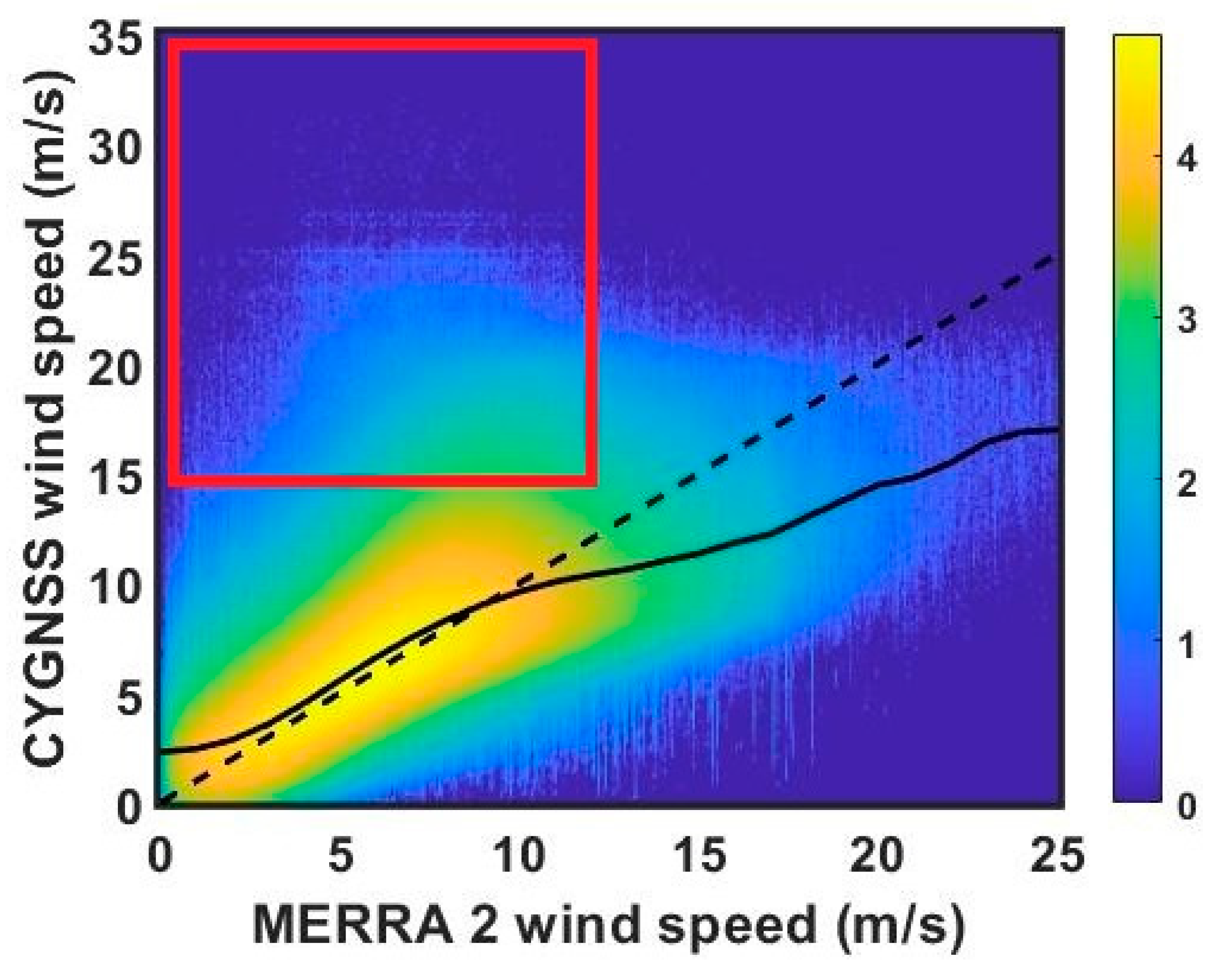At Level 2, the quality flags look out for retrieval ambiguity, low Range Corrected Gain (RCG) and other data processing errors [11]. Despite such stringent quality flags in place, there remain occasional outlier samples with large discrepancies between the CYGNSS retrieved wind speed and reference validation winds (shown in Figure 1) To improve the data quality of CYGNSS, another layer of quality control is needed which can effectively identify and eliminate these outliers. This is the primary objective of this work.

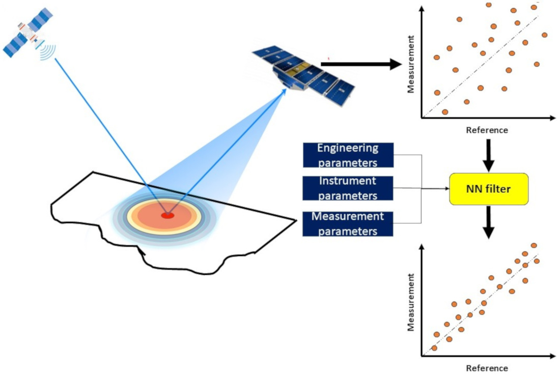
In this work we develop a Neural Network based quality control filter for CYGNSS Level 2 winds which can effectively identify and remove outliers. We also consider the performance of the CYGNSS retrieved winds before and after this filter is applied to assess its efficacy. The reminder of the paper is structured as follows. Section 2 describes the datasets used. Section 3 explains the details of the proposed quality control filter. In Section 4 the performance of the proposed algorithm is analyzed and the CYGNSS level 2 data performance is assessed before and after the filter. Section 5 discusses the trade-offs in performance and conclusions of this study.

2. Data Description

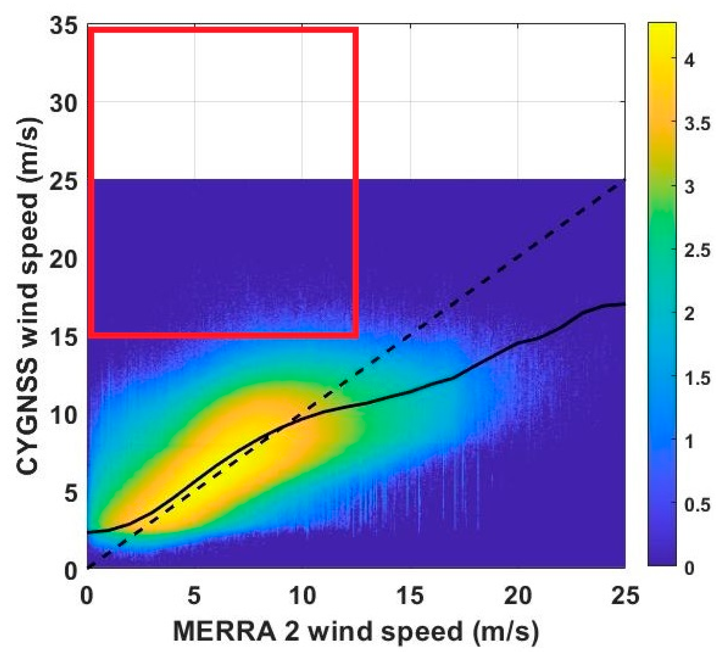
The Level 2 CYGNSS winds are minimum variance estimated winds from two observables namely, NBRCS and LES for low-moderate wind speed ranges (0–25 m/s). The CYGNSS retrieved winds are matched to near coincident independent estimates of the ocean surface wind speed referenced to a 10 m height ($u_{10}$) from the Modern-Era Retrospective Analysis for Research and Applications, version 2 (MERRA-2) [12]. MERRA-2 is a reanalysis product provided by NASA’s Global Modelling and Assimilation Office (GMAO). The reference matchup MERRA-2 gridded data product has a spatial resolution of 0.5 deg × 0.625 (lat, lon) and an hourly instantaneous assimilation [13].

Figure 1 shows the density scatter plot of CYGNSS retrieved winds with respect to the MERRA-2 winds. In the figure, the dashed line represents the 1:1 line and the solid line represents the mean retrieved wind speed line, which essentially is the GMF. This plot is generated by dividing the 2-D space into 500 bins or regions. And the matchup winds are assimilated into the nearest bin and finally the log to the base 10 of the number density is taken for better visualization of the density differences. There are several important observations from this plot. Firstly, most of the observations fall along the 1:1 line at lower wind speeds, indicating good retrieval quality. However, a cluster of very high CYGNSS retrieved winds (15–35 m/s) is noticeable at low MERRA-2 winds (5–10 m/s). The improved filtering method developed here targets the removal of these outliers. Secondly, the GMF line and the 1:1 line are very similar up to a MERRA-2 and CYGNSS wind speed of ~10 m/s. Above this range, the GMF line begins to deviate away from the 1:1 line. This inherent bias in the GMF complicates the identification of outliers by the filter algorithm. The purpose of a quality filter is to remove outliers only and not correct for biases in the retrieval. This is another consideration to be accounted for while designing the filter. Finally, the density of samples at high MERRA-2 wind speeds (>20 m/s) is very small relative to the lower wind speed ranges. Therefore trade-off studies must be performed for filter design to balance between efficiency of outlier removal and retaining as many high wind samples as possible. All the above objectives will be addressed in the course of developing the filter.

Over and above the existing quality flags, 13 diagnostic variables are used to distinguish outlier samples from good samples. These diagnostic variables are listed in

Table 1. List of diagnostic variables used.

Diagnostic Variable	Description	Type	Symbol/Abbreviation
prn_code	GPS PRN code	Instrument attribute	PRN
antenna	CYGNSS science antenna	Instrument attribute	ant
nst_att_status	Star tracker attitude status	Instrument attribute	nst
sc_roll	Spacecraft roll	Instrument attribute	Roll
zenith_ant_gain	Zenith antenna Gain	Instrument attribute	$Z_{gain}$
zenith_power	Zenith antenna power	Instrument attribute	$Z_{power}$
incidence_angle	Incidence angle at SP	Geometry attribute	$\theta$
azimuth	Azimuth angle of SP	Geometry attribute	$\phi$
range_corr_gain	Range Corrected Gain	Geometry attribute	RCG
sp_rx_gain	CYGNSS antenna Gain at SP	Surface attribute	G
ddm_snr	SNR at SP	Surface attribute	SNR
ddm_nbrcs	NBRCS at SP	Surface attribute	DDMA
ddm_les	LES at SP	Surface attribute	LES

SP = Specular Point.

. The choice of diagnostic variables is based on previous calibration experience with GNSS-R data and error analyses [7,8,9]. The diagnostic variables can be categorized into 3 major types—instrument related attributes, measurement geometry related attributes and surface related attributes. In Section 4 these diagnostic variables will be assessed for their individual significance in enabling the filter to distinguish between outliers and good samples.

3. Proposed Quality Control Method

Outlier/anomaly detection is an active research field spanning a wide range of applications from manufacturing quality control to astronomical detections. Machine learning techniques are widely used for outlier detection and automation of quality control processes [14]. Despite an emerging trend in the use of machine learning methods for Earth Observation applications, the calibration and validation of satellite measurements are most often handled manually by instrument specialists. Utilizing the capabilities of machine learning tools for calibration and validation activities can help to better understand the behavior of the data.

Outliers can be defined as sample measurements that have a distinct deviation in their properties when compared to the major proportion of the data [15]. Visually, these measurements are regions of low density in the sample space, i.e., have a significantly low number of neighboring points within a threshold distance compared to rest of the sample space. Machine learning tools that are widely used for outlier analysis includes the supervised classification techniques such as Neural Networks (NN), K-Nearest Neighbors (K-NN), Decision trees, Support Vector Machines (SVM) etc. [16]. As noted in Figure 1, there are distinct regions away from the GMF line and the 1:1 line which should be detected and removed. For the CYGNSS quality control filter, supervised training of a Neural Network is used for outlier detection and removal. The details of the quality control filter design are explained in this section.

3.1. Population Definitions

The CYGNSS Level 2 v3.0 data with MERRA-2 wind speed matchups from the year 2018 have a total of ~153 million samples. The sample space is divided into 2 regions. The low wind region consists of all samples with CYGNSS retrieved winds, $U_{CYG}$, less than or equal to 10 m/s. The high wind region consists of samples with $U_{CYG}$ greater than 10 m/s. In both regions MERRA-2 wind speed, $U_M$ is required to be less than 25 m/s. This division of sample space is due to the behavior of the GMF line relative to the 1:1 line. Below 10 m/s, the GMF line is very similar to the 1:1 line (see Figure 1) and above this wind speed the GMF line begins to underestimate. Therefore, it is appropriate to have two different training datasets, one for each region.

In the low wind region, a good sample satisfies $\left|U_{CYG}- \langle U_{CYG}\rangle {|}_{U_M}\right|\le$ 1 m/s. and an outlier satisfies $\left|U_{CYG}- \langle U_{CYG}\rangle {|}_{U_M}\right|>$ 4 m/s, where $\langle U_{CYG}\rangle {|}_{U_M}$ refers to the mean value of the wind speed retrieved by CYGNSS for a given value of the MERRA-2 wind speed. This relationship is described by the solid line in Figure 1. In the high wind region, a good sample is defined by $\left(U_{CYG}-U_M\right)\le 2 \mathrm{m}/\mathrm{s}$ and an outlier as a sample $\left(U_{CYG}-U_M\right)>3 \mathrm{m}/\mathrm{s}$. 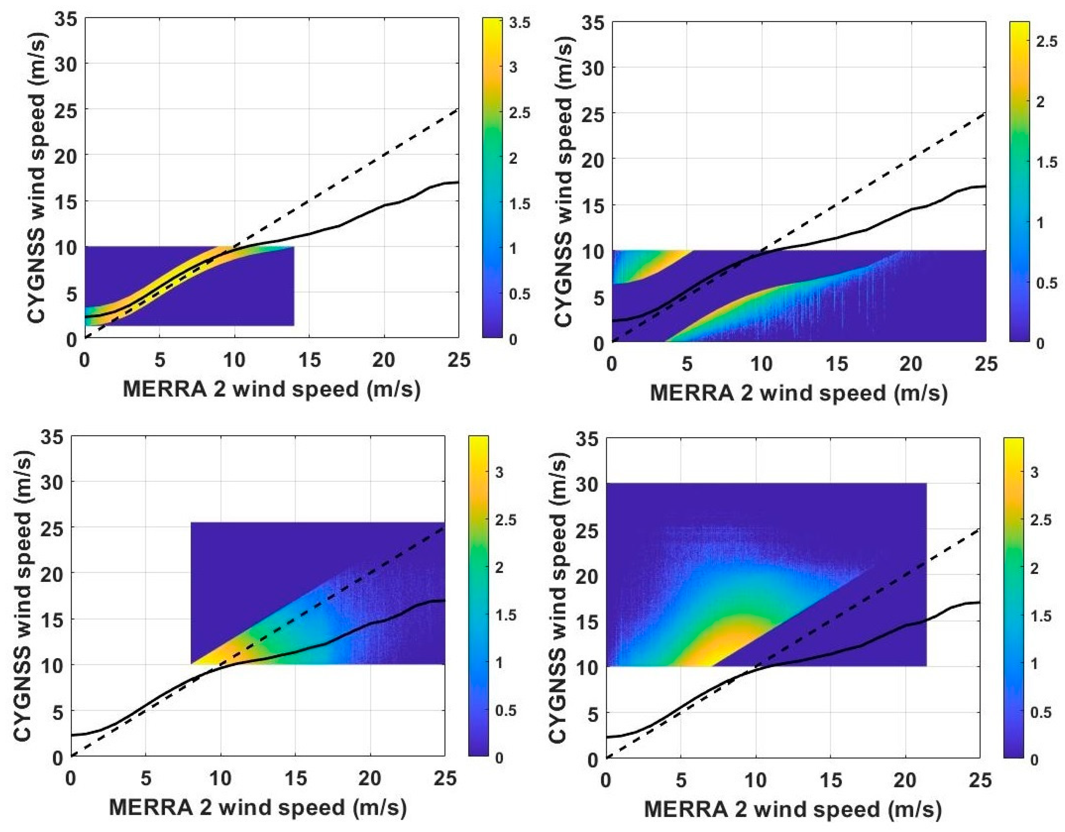The difference in training population definitions at low and high wind speeds is due to the inherent bias in the GMF which can be observed as the deviation of the retrieval mean (solid line) from the 1:1 agreement (dashed line) above 10 m/s in Figure 1. As the wind retrieval is based on the GMF, a bias in the GMF can lead to under/over-estimation of winds despite being a good measurement. To mitigate the effect of GMF-induced bias on the outlier detection capability of the filter, the filter is trained with respect to the GMF. However, as the filter is reliant on the Level 1 diagnostic variables which are independent of GMF, the samples lying near the 1:1 line are also good samples and therefore the modified definition of training data is used at high winds. The training datasets for the 2 different sample spaces are shown in Figure 2. Such conservative training definitions are used to improve the outlier detection capability of the algorithm. Further analysis of the definition of a good or an outlier sample is discussed later in this section. For training, we use ~4 million samples for each wind speed region and ~8 million samples for validation. The performance metrics used to evaluate the outlier detection capability of an algorithm are the Probability of Detection (PD) and False Alarm Rate (FAR). For these metrics, the definition of good and outlier samples are different from the training definitions. The validation definitions are based on the NASA mission requirements on wind retrieval error. Thus, the wind speed differences for a good sample shall be less than 2 m/s from the mean and an outlier is defined as those samples having a difference greater than 5 m/s. Finally, the filter is tested over the total population and its performance is assessed.

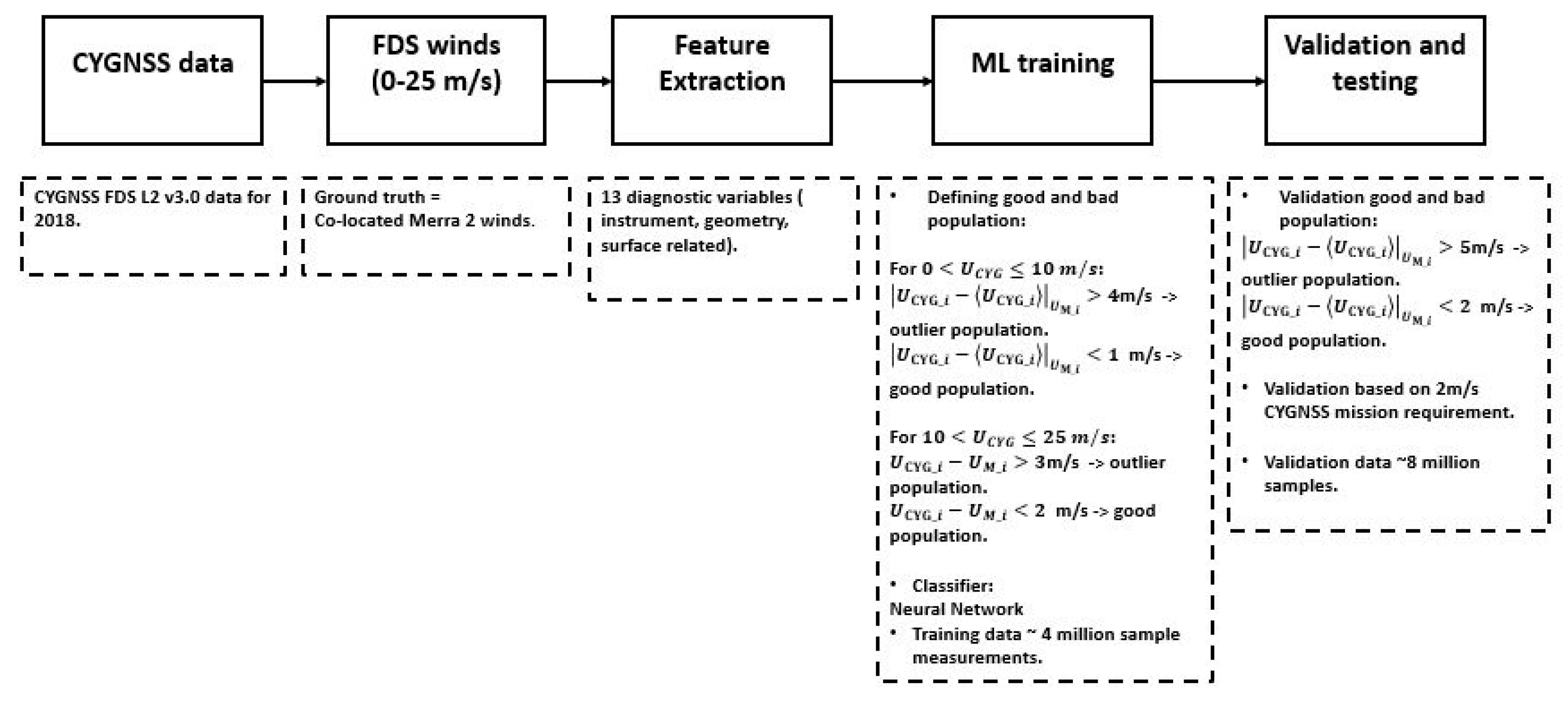
3.2. Quality Control Process Design

A block diagram representation of the quality control design process is shown in Figure 3. The first stage of the algorithm is feature extraction. The input to this stage is the Fully Developed Seas (FDS) winds over a reference wind speed region of 0–25 m/s. The CYGNSS Level 2 wind retrievals are of two kinds—the FDS and Young Seas Limited Fetch (YSLF) winds. The FDS winds are low to moderate winds (up to 25 m/s) over fully developed waves in the ocean. This forms the major proportion of the total measurements. The YSLF winds are hurricane force winds measured over the tropical cyclones that have varying wave age and fetch conditions. The filter proposed in this work is developed specifically for FDS winds as this dataset encompasses the majority of the measurements and have a well behaved nature relative to its counterpart. The feature extraction stage extracts the different diagnostic variables listed in Table 1 for every sample point. Next is the training stage. One Neural Network (NN) classifier is trained for each of the wind speed space over the individual training datasets described above. The last stage is the validation and testing stage where the skill of the filter is assessed. The performance assessment of this Neural Network filter is discussed in detail in Section 4.

Apart from the Neural Network filter, other standard supervised outlier detection techniques such as Logistic Regression, Decision Trees, Naïve Bayes and K-NN are also considered and their confusion matrices are listed in

Table 2. Training time required for individual classifiers (top). Confusion matrices for different classifiers (bottom).

Classifier	Training Time (secs)
Logistic Regression	118.43
Decision tree	78.87
Naïve Bayes	56.39
K-NN	49,608 (13.78 h)
NN	6475 (1.8 h)

(bottom). In the confusion matrix, the rows represent the true classes, the columns represent predicted classes, and the percentage of samples are mentioned in each of the boxes. Outliers are represented as class ‘0’ and good samples are represented as class ’1’. Among the various classifiers experimented with, the K-NN and the NN have a similar performance. In general, NN is preferred over K-NN because of the heavy computational memory requirement of K-NN as compared to the memory requirement for training the NN coefficients. This can be seen in terms of the time requirement for training each of the classifier, shown in Table 2 (top). It can be seen that K-NN requires the most time, followed by the NN.

3.3. Neural Network Filter Design

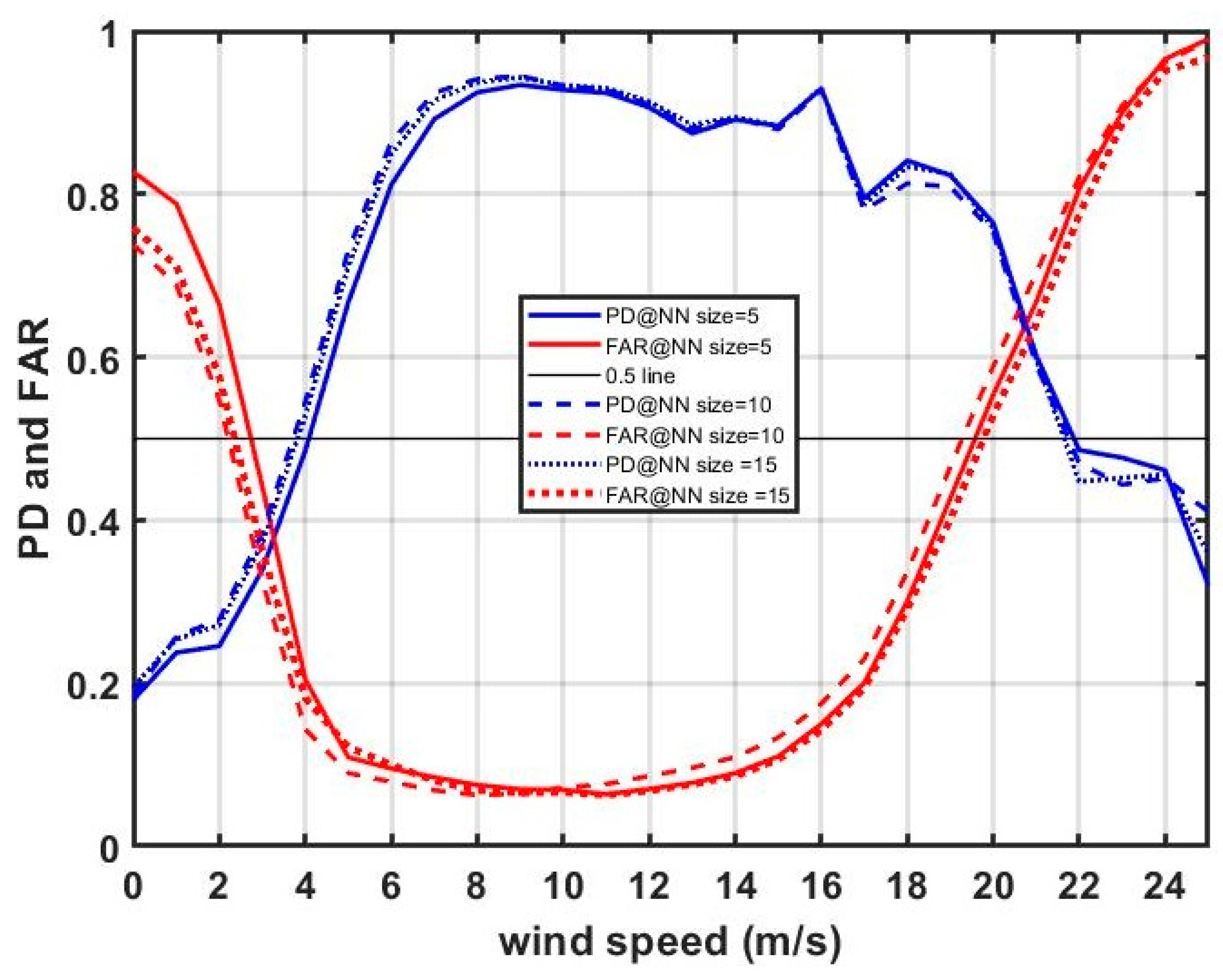
The NN used for this application consists of a single hidden layer with 10 neurons. The input layer consists of 13 neurons, each for one diagnostic variable and the output layer has one neuron that classifies an input sample as an outlier or a good sample. Only one hidden layer is used as it is a sufficient condition to form any bounded/unbounded convex region in the space spanned by the input [17]. The choice of the number of neurons in the hidden layer is decided by experimentation. In general, a feedforward network can have any shape but the commonly used structure is a pyramidal structure with decrease in number of neurons at each layer away from the input. There is practically no upper limit on the number of neurons to be used in this case as the training population is very high (~4 million). So, 3 different neurons counts are experimented here and the performance plot in terms of PD and FAR at different wind speeds is plotted to make a choice on the hidden layer size. The performance plot is shown in Figure 4.

The blue curves represent PD and the red curves represent FAR. It can be noticed that all 3 network sizes have a very similar performance in terms of PD and FAR over the entire wind speed range. For this reason, other performance metrics such a computation time, network complexity and % samples removed as outliers are considered when choosing the optimal structure. In terms of computational time, NN size = 15 is the shortest, followed by NN size =10, and the longest is NN size = 5. This is an expected trend, as simpler networks can take larger time for error convergence. Next, in terms of network complexity, NN size = 5 has the least number of tunable parameters, followed by NN size=10 and the largest being NN size =15. The % of samples removed as outliers by NN size = 5 is ~ 23% of the total data, by NN size =10 is ~ 20% and by NN size = 15 is ~22%. Therefore, after all these considerations, NN size=10 is chosen as the optimal network design for this application.

Thus for purposes of quality control application for CYGNSS, the QC filter has two NNs (NN1 and NN2), each trained for a specific wind speed range (0–10 m/s and 10–25 m/s). The NNs are identical in architecture and contain 2 layers with 10 neurons in the hidden layer, as discussed above. The hidden layer is trained with a sigmoid transfer function and a linear transfer function is used in the output. The optimization algorithm used for this is the widely used Levenberg-Marquardt algorithm.

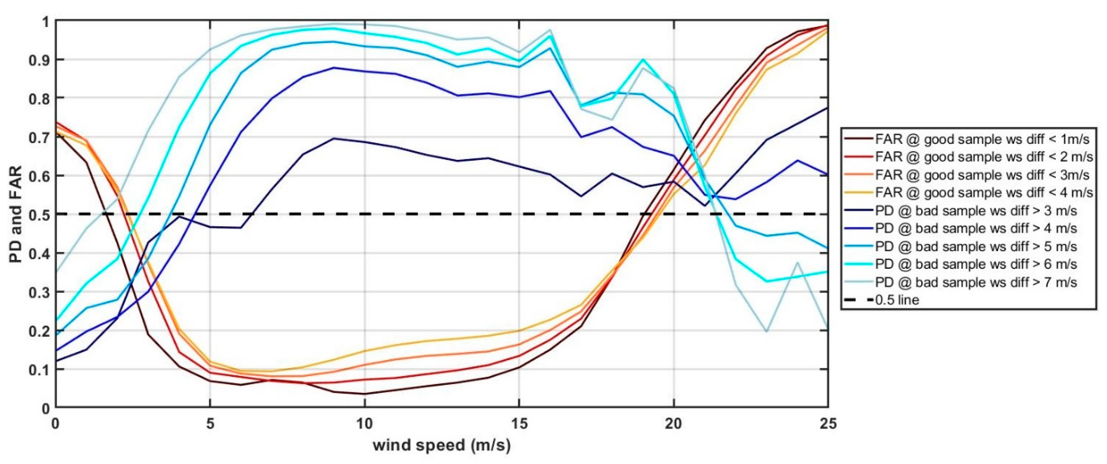
To evaluate the design space of this filter, the definitions of good and outlier samples are varied and the performance metrics are plotted. Understanding the behavior of the filter for different sample definitions can help users understand how the network handles the outliers and choose an optimum definition based on the application requirements. The family of PD and FAR curves are plotted in Figure 5. The blue curves represent PD and red curves represent FAR. The PD metric is affected by the density of outlier samples and the FAR metric is affected by the density of good samples. Changing the wind speed difference thresholds for good and outlier samples will affect the overall performance of this QC filter. For this study, the wind speed difference from the GMF line for a good sample is varied from 1 m/s to 4 m/s and for an outlier is varied from 3m/s to 7 m/s.

There are many interesting features in Figure 5. Firstly, the FAR curves do not vary much with changes in the definition of the good population but there is a significant jump in PD with changes in the definition of the outlier population. This is due to the relatively small percentage of outliers when compared to the total sample population. Next, the FAR metric has the best performance when the good sample definition is set to 1 m/s and gradually degrades with increase in the difference. However, above a wind speed of ~18 m/s, the trend reverses. This is due to the fact that, at higher wind speeds there is a greater degree of scatter in the data (as seen in Figure 1) resulting in poorer performance in terms of FARs at very stringent definitions of a good sample. Next, as mentioned earlier, the PD metric seems to have a strong jump with change in outlier definition; with the highest PD performance for an outlier definition of >7 m/s for wind speed difference from the GMF line. Again, the trend flips in nature at higher wind speed (>21 m/s), this is again attributed to increased scatter in the data. Finally, it is important to note that the general performance of the filter is not optimal at very low wind speeds (<3 m/s) for any definition of good and outlier sample. Thus, the ideal operating range for this filter is ~5 m/s to 18 m/s; this were most of the samples lie. The choice of the definitions is dependent on the application. For instance, applications that require very high quality control like monitoring long term variations in wind speed data must go for highest PD performance. Applications at higher wind speeds which needs to retain as many higher wind speed samples as possible, must go for lower PD performance. In this work the assessment of wind retrieval performance is used as its definition of good sample a wind speed difference <=2m/s and defines outliers as >5 m/s.

4. Results

In this section the performance of the quality controlled CYGNSS wind speed data set is assessed. Two identical Neural Networks, one for each wind speed region discussed in Section 3 are trained. The first NN is applied to CYGNSS winds between 0–8 m/s and the second NN is applied to CYGNSS winds >8 m/s. This slight shift between the training and testing wind speed regimes is to improve the net performance of the filter, as the first NN will be biased towards the lower winds where the highest density of samples are present and the second NN will again be biased towards the lower winds in its range (10–35 m/s). The resulting quality controlled CYGNSS wind speed dataset is shown in Figure 6.

Comparing Figure 1 and Figure 6 demonstrates the effectiveness of the filter. The large cluster of high CYGNSS winds at low MERRA-2 winds has been removed by this filter (compare the red box region between the two figures). Also, the CYGNSS samples are now evenly distributed along the GMF line (solid black line) unlike in the original dataset. Finally, a significant reduction of scatter in the dataset can be observed. The performance of this proposed QC filter is assessed in the following subsections based on the error statistics Mean Difference (MD), Root Mean Squared Difference (RMSD) and variance of data. The test dataset consists of all the sample points (~153 million).

4.1. Algorithm Performance Analysis

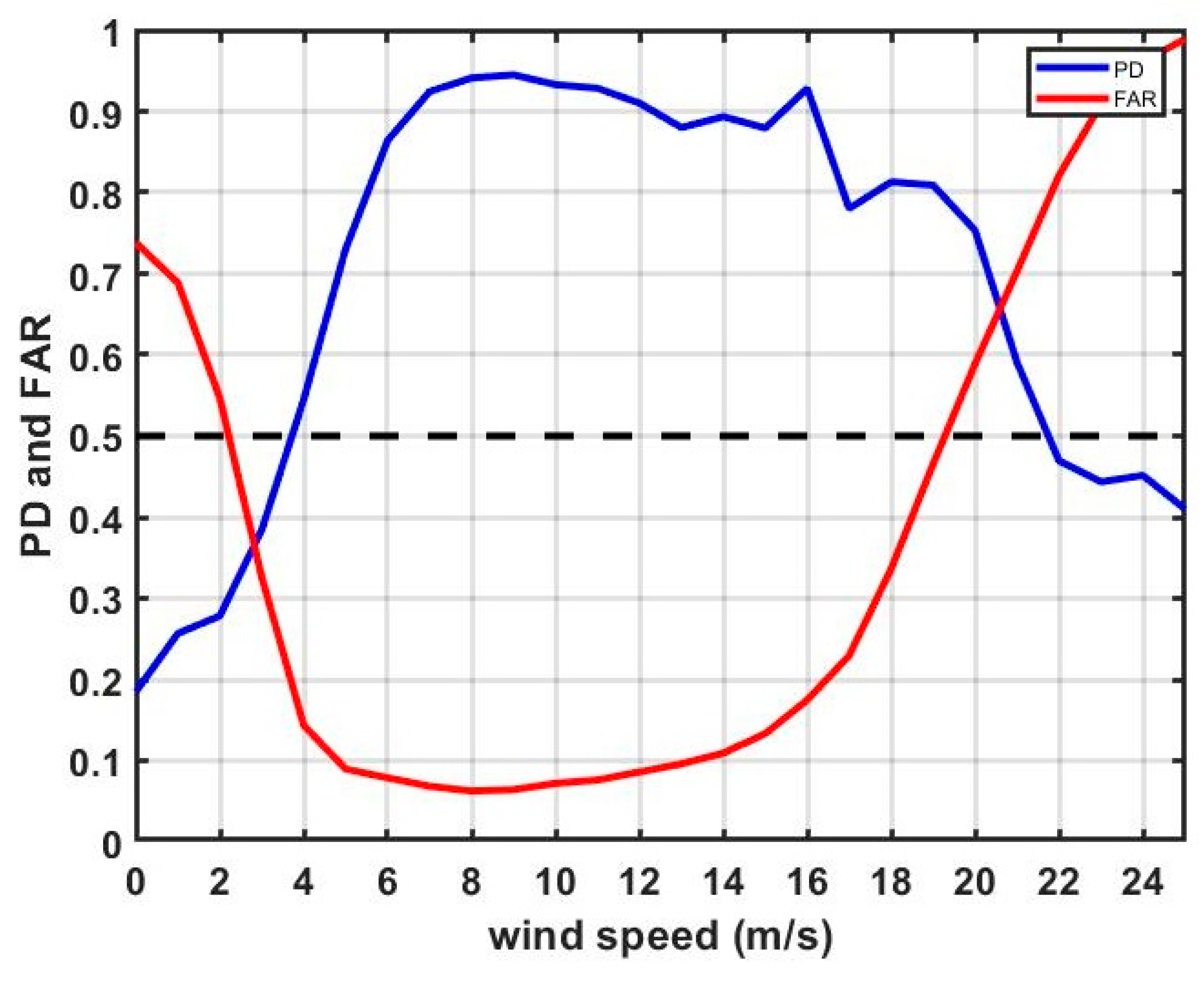
To assess the skill of the quality control algorithm, first the validation metrics, PD and FAR, are examined in Figure 7. These metrics are based on the design parameters discussed in the previous section. The optimal range of operation for this filter is ~5 m/s to 17 m/s. In this range the FAR for good samples is consistently <20% and the PD for outliers is >75%. The peak performance is between 6–14 m/s where FAR <10% and PD is >80%. This is also the region of maximum data density as the wind speed distribution has a peak near 7 m/s.

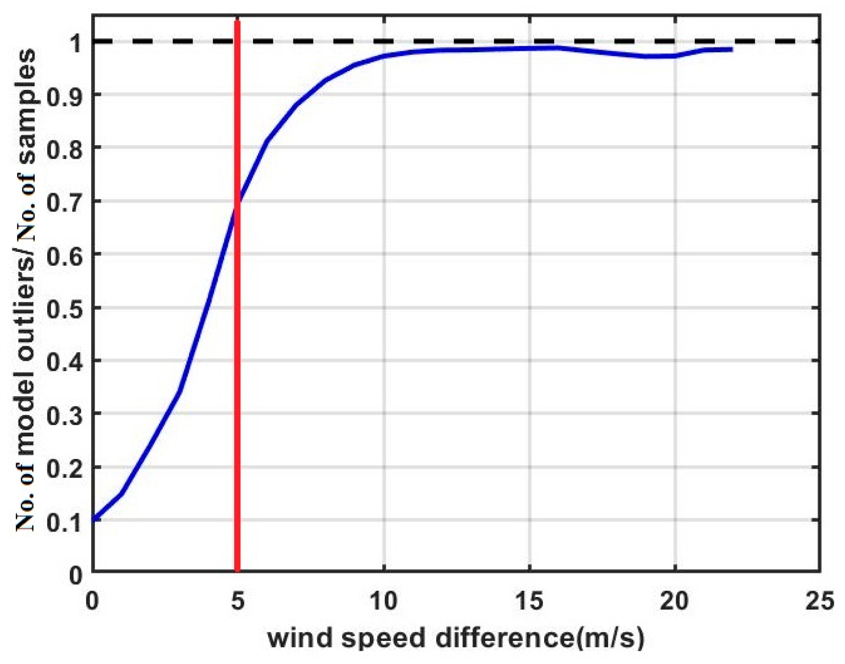
Next, the skill of the filter is assessed by looking at the ratio of number of outliers identified by the filter to the total number of outliers for a range of wind speed differences. This is shown in Figure 8. The x-axis is the difference between CYGNSS wind speed and the GMF line. As per our validation criteria, we have defined any sample as an outlier if the difference is greater than 5 m/s. The 5 m/s threshold is shown in red. It can be observed that ~70% of the outliers are rightly identified for wind speed difference ~ 5 m/s and the filter eliminates close to ~100% of outliers with wind differences >10 m/s.

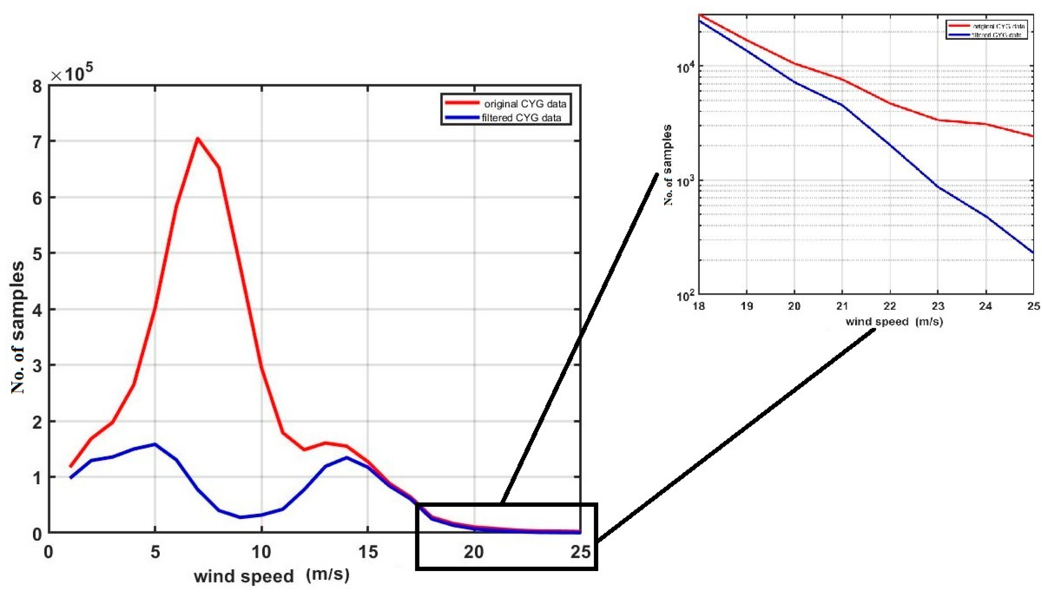
To understand Figure 8 better, we look at the distribution of outliers (wind speed difference >= 5 m/s) at different MERRA-2 wind speed bins before and after applying the filter. This data distribution is shown in Figure 9. The red distribution shows the density of outliers in the original dataset and the blue shows the distribution of outliers after applying the filter. Firstly, a very significant decrease in the outlier population can be observed after filtering. The filtered dataset has approximately 4 times less outliers. In the original dataset, most of the outliers are present between 5–10 m/s which is also the peak region for wind speed distribution. In this region the filter has been able to remove a large proportion of the outliers. Next, in the filter design section the low PD and high FAR at high winds region was discussed. Though at first, it may appear as if the filter cannot operate in this wind speed region, the distribution of outliers in this region (plot on the top right) shows that the number of outliers is almost an order of magnitude smaller after the filtering process, indicating that the filter can operate efficiently in this region but the low sample density in the region does not reflect this capability of the filter in the PD and FAR metrics.

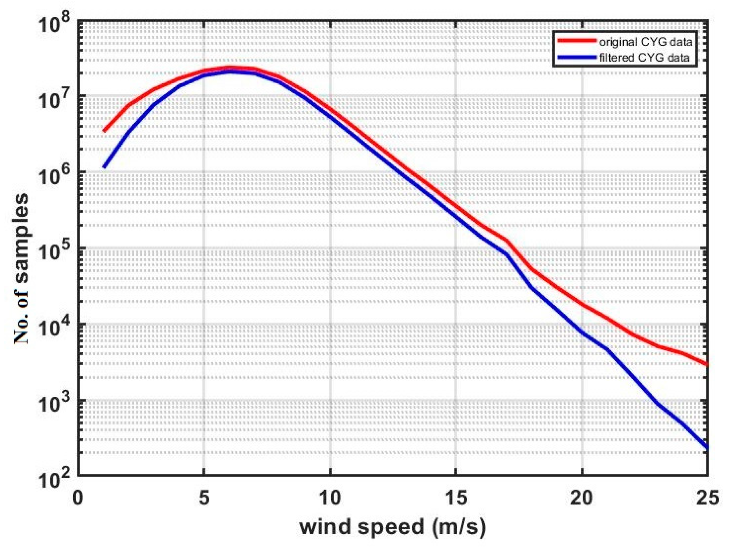
Finally, the total wind speed distribution of the dataset before and after applying the filter is plotted in Figure 10. After applying the filter, ~20.5% of the data have been removed by the filter as outliers. From Figure 10 it can be observed that the largest difference in density occurs at high wind speeds (>18 m/s). This is partly due to the high FAR of the filter in this region and partly due to large scatter in the data in this region. A substantial difference in density can also be observed at very low wind speed regions (<3m/s), again owing to the high FAR of the filter in this region.

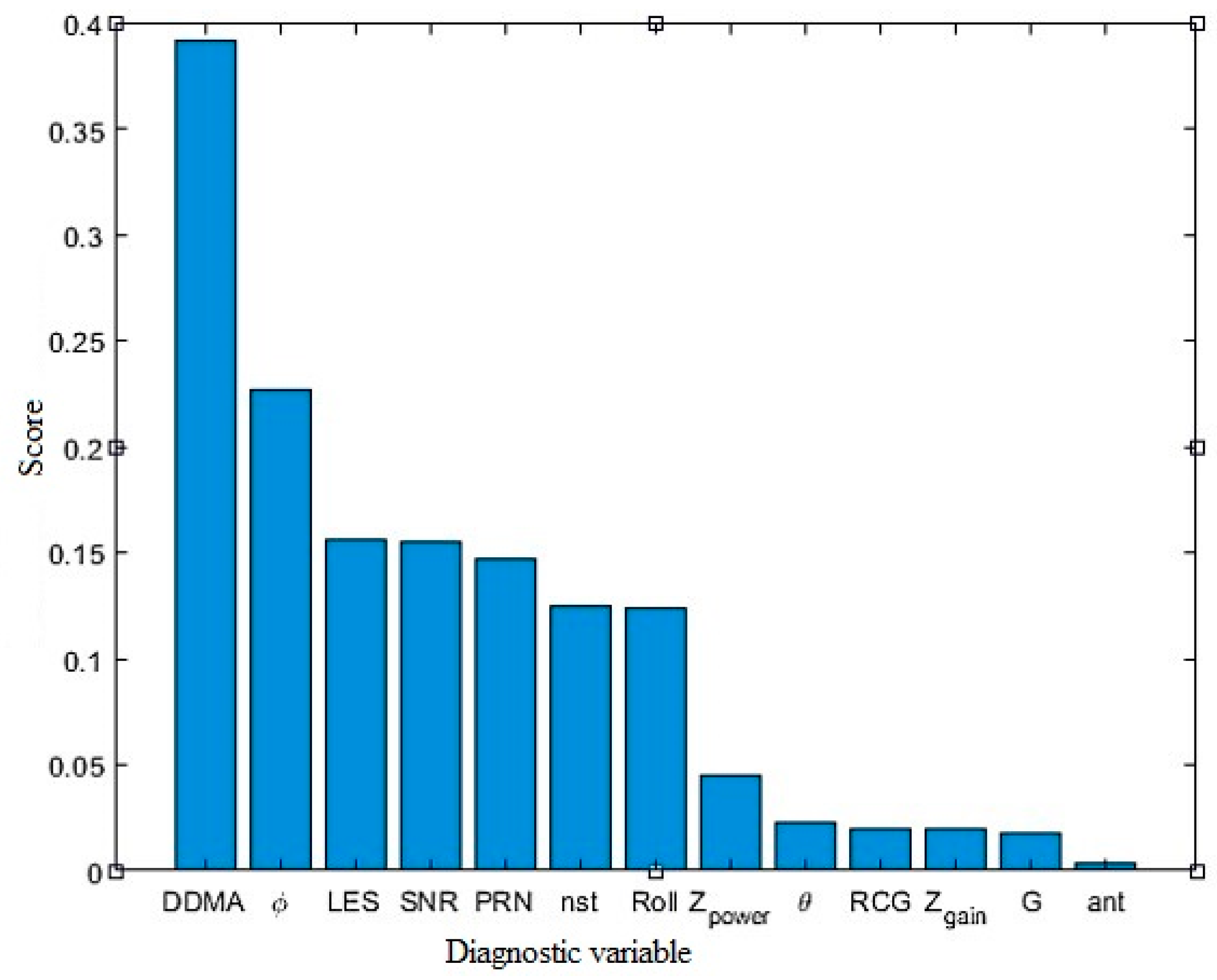
4.2. Identifying Dominant Feature Vectors

In this section the importance of each of the diagnostic variable is assessed using the minimum redundancy maximum relevance algorithm. The algorithm minimizes the redundancy of the feature set and maximizes the set with respect to the training data. Pairwise mutual information of the diagnostic variables is used to quantify its redundancy and relevance [18]. Figure 11 shows the score for each of the variable based on its importance in distinguishing outliers from good samples.

The most dominant feature is the DDMA (NBRCS). This is as expected because the wind retrieval by CYGNSS is directly related to the two observables NBRCS and LES. The other dominant features are pre-dominantly instrument related such as azimuth angle, PRN, star tracker attitude status and satellite roll. This suggests that most of the outliers are caused due to improper instrument calibration.

4.3. Wind Retrieval Performance

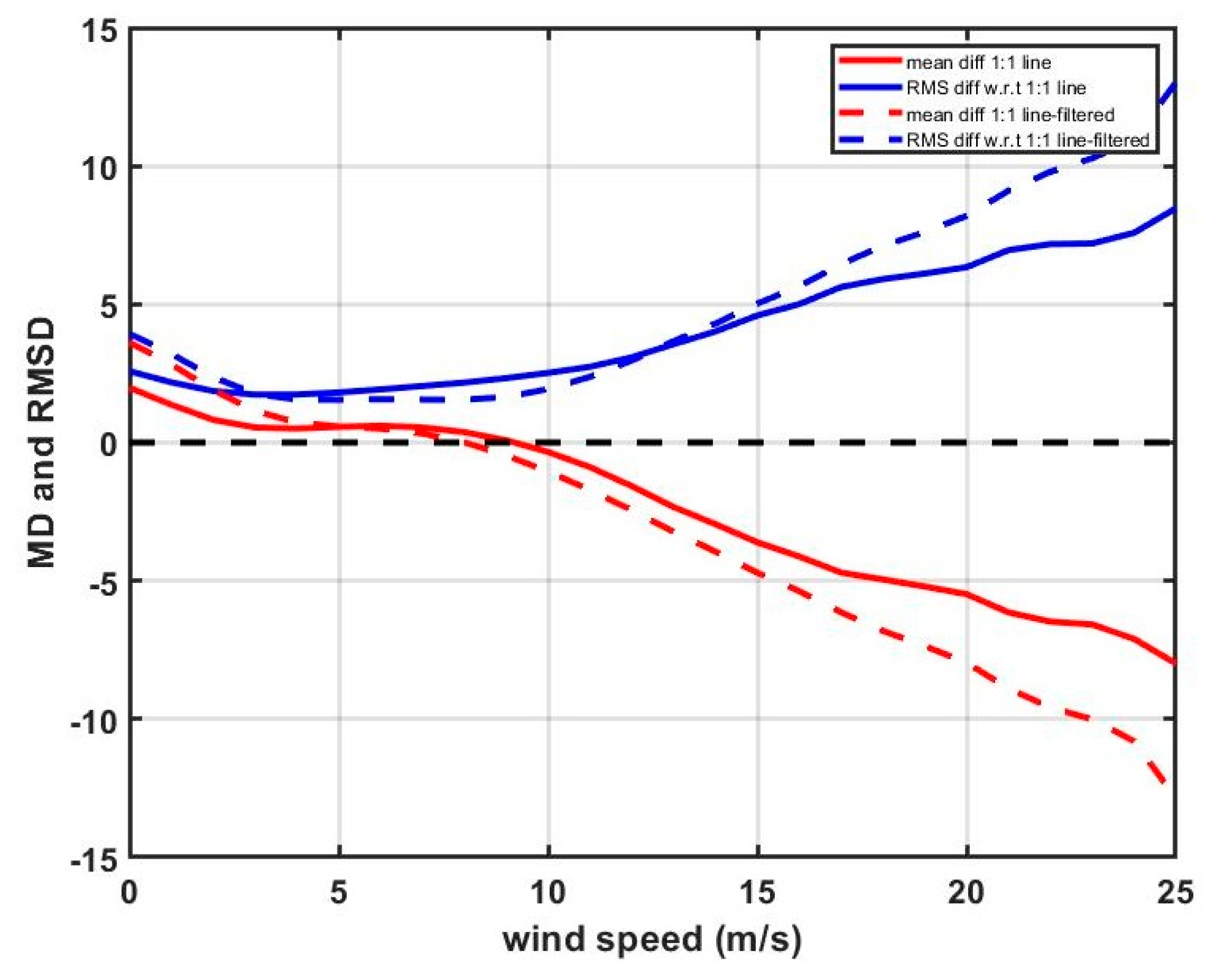
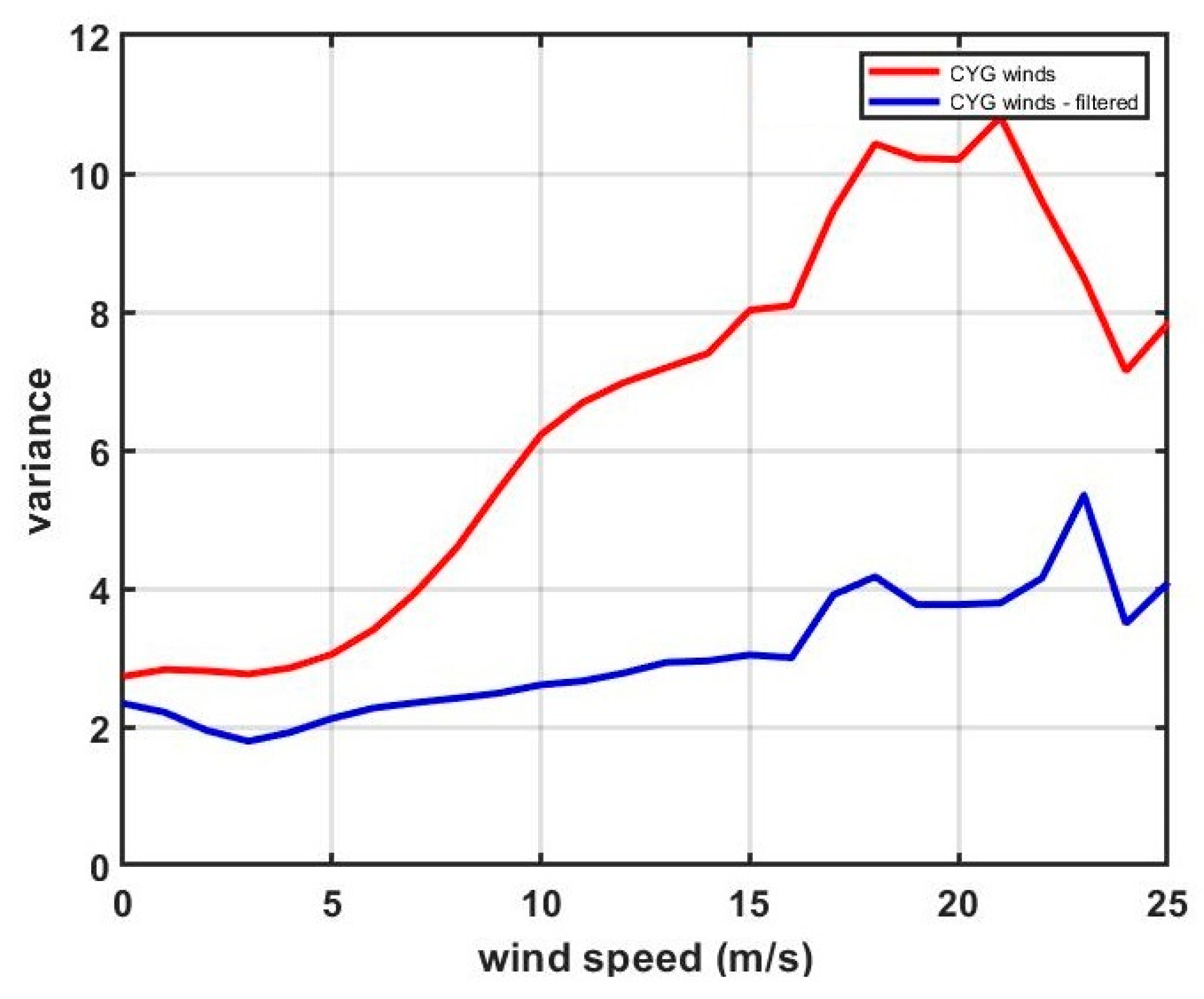
The CYGNSS wind retrieval is evaluated based on 3 error statistics, namely, the Mean Difference (MD), RMS difference (RMSD) and variance in the data. The MD and RMSD are evaluated with respect to the 1:1 line thus is a superposition of both variance in the data and the intrinsic bias in the GMF. Whereas the variance is a measure of only the degree of scatter in the data. The error statistics are presented in Figure 12 and Figure 13. In Figure 12 the MD and RMSD of the original dataset is shown by solid lines and the filtered dataset is shown by dashed lines. An increase in bias can be observed in the filtered dataset as compared to the original dataset; this is because, after filtering the samples that are identified as good by the filter are aligned closer to the GMF line rather than the 1:1 line. The increase in bias is more dominant above 10 m/s as the GMF line begins to deviate away from the 1:1 line above this wind speed. Figure 13 shows the variance in the data at different wind speed bins. Variance represents the degree of scatter in the data and after applying the filter there is a sharp drop in the scatter. The standard deviation in the filtered dataset is <=2 m/s for a wide range of wind speeds. These error statistics show a significant improvement in the nature of retrieval after the QC filter.

5. Discussion

The CYGNSS retrieved winds are currently being used for various ocean science applications such as ocean circulation studies, regional and global analysis of ocean winds [19], tropical cyclone studies [20,21,22,23], and assimilation into Numerical Weather Prediction (NWP) models. Data reliability plays an important role in aiding such scientific studies. The CYGNSS wind speed data products are of two kinds—the Fully Developed Seas (FDS) wind retrievals and Young Sea Limited Fetch (YSLF) retrievals. Of these two, the FDS winds form the major proportion of the measurements and are therefore used for many scientific applications, especially for assimilation into NWP models. The YSLF data product is for hurricane force winds measured over individual storms, therefore is a substantially smaller set of measurements. The QC mechanism developed in this work is for the CYGNSS FDS winds, in order to reduce errors (in particular, outliers) in the retrieval due to various engineering and measurement related errors.

The primary merit of the proposed ML filter is its ability to better account for interactions between the individual engineering, instrument and measurement conditions than can separate thresholded flags for each one. The current approach upon which we are improving uses individual flags and, despite these existing QC filters, there remains considerable scatter in the data—hinting that individual and independent thresholds is not an effective way of removing the outliers.

The filter proposed here utilizes the capability of ML tools to learn inherent patterns from the training dataset and quickly come up with any convex boundaries separating the outliers from good data. One other advantage of such filters is that, because the system itself is aging with time, and as shown in this work—most of the outliers are due to calibration errors, the new ML-based QC thresholds can be reassessed periodically. In such situations, the ML filters come in handy as their parameters can be tuned easily to respond to any changes.

Assimilating the CYGNSS near surface wind retrievals into NWP models for better forecasting is one of its important uses. In general, NWP models give a weight to meteorological satellite observations based on their error statistics. Thus, reducing errors in the retrieval will help assimilate CYGNSS winds better. Using this filter, the standard deviation of the retrieval is reduced from 2.6 m/s to 1.7 m/s over the wind speed range 0–25 m/s.

At higher wind speed ranges, this filter is too aggressive and removes some valuable high wind measurements. This is due to the fact that high wind data density (> 20 m/s) is very sparse, hence insufficient for the Neural Network to be able to learn significant patterns from it. To address this situation, one possibility is to assimilate more of CYGNSS high wind data in future years, to better train the Neural Network in this region. However, it is also important to consider here that the CYGNSS FDS winds are reliable only up to 25 m/s as they have been developed using NOAA/GDAS ocean surface winds as their reference [24].

The direction of focus of future work will be to develop automated machine learning based QC that can effectively remove outliers at all wind speed ranges. Currently this filter is operable only between 5–18 m/s. The lower sample density at high and very low winds, prevent the QC filter from operating in these regions. One possible solution, as mentioned above, is to wait for more CYGNSS measurements in these wind speed regions before the QC is applied. Using ML based QC for YSLF winds can be complicated by the rapidly varying sea state inside hurricanes. In such cases, a physics based definition of an outlier might be needed. One approach to apply quality control for such data is to observe trends along overlapping tracks within a given spatial boundary around the hurricane.

6. Conclusions

In this work a Neural Network based Quality Control filter for CYGNSS wind retrieval is developed. The inputs to this filter are the 13 diagnostic variables that broadly represent instrument related, measurement geometry related and surface related attributes. Of these diagnostic tools, the surface related attributes (NBRCS, LES, and SNR) and instrument related attributes (azimuth angle, star tracker status, PRN, satellite roll) play a dominant role in distinguishing outliers from good sample population. The Neural Network is trained over two different training datasets at two different CYGNSS wind regimes based on the behavior of the GMF. The operating range of the filter is between 5–18 m/s. Within this range the probability of outlier detection is > 75% and the false alarm rates is <20%. In total ~20.5% of the data is removed as outliers by this filter. Atleast 75% of the outliers with wind speed difference of at least 5 m/s is removed while ~100% of the outliers with wind speed difference of at least 10 m/s is removed. This filter has significantly reduced the scatter in the data. The quality filtered dataset has a standard deviation of <=2 m/s over a wind range of wind speeds. The design space for this filter is also analyzed in this work to identify trade-offs between PD and FAR. The choice of PD and FAR will depend on the application. For example, a low FAR may be especially important for applications in which good spatial and temporal sampling are very important (e.g., to image rapidly changing weather systems) whereas a high PD may be especially important for applications in which the lowest possible uncertainty in wind speed is important (e.g., to detect small trends over long time intervals, such as are associated with global change).

As the next steps in this work, the higher wind regime will be the focus of interest. Strategies to improve the performance of this filter at higher winds while retaining as many samples as possible will be considered. Also, currently this filter is developed only for fully developed seas, in the future the feasibility of extending to young seas will also be studied.

References

- Clarizia, M.P.; Gommenginger, C.P.; Gleason, S.T.; Srokosz, M.A.; Galdi, C.; Di Bisceglie, M. Analysis of GNSS-R delay-Doppler maps from the UK-DMC satellite over the ocean. Geophys. Res. Lett. 2009, 36. [Google Scholar] [CrossRef] [Green Version]
- Gleason, S. Space-Based GNSS Scatterometry: Ocean Wind Sensing Using an Empirically Calibrated Model. IEEE Trans. Geosci. Remote. Sens. 2013, 51, 4853–4863. [Google Scholar] [CrossRef]
- Unwin, M.; Duncan, S.; Jales, P.; Blunt, P.; Brenchle, M. Implementing GNSS Reflectometry in Space on the TechDemoSat-1 Mission; Procedings Institute Navigation: New York, NY, USA, 2014; pp. 1222–1235. [Google Scholar]
- Ruf, C.; Chew, C.; Lang, T.J.; Morris, M.; Nave, K.; Ridley, A.; Balasubramaniam, R. A New Paradigm in Earth Environmental Monitoring with the CYGNSS Small Satellite Constellation. Sci. Rep. 2018, 8, 8782. [Google Scholar] [CrossRef] [PubMed] [Green Version]
- Ruf, C.; Chang, P.; Clarizia, M.P.; Gleason, S.; Jelenak, Z.; Murray, J.; Morris, M.; Murray, J.; Musko, S.; Posselt, D.; et al. CYGNSS Handbook; United States of America by Michigan Publishing: Ann Arbor, MI, USA, 2016. [Google Scholar]
- Clarizia, M.P.; Ruf, C. Wind Speed Retrieval Algorithm for the Cyclone Global Navigation Satellite System (CYGNSS) Mission. IEEE Trans. Geosci. Remote. Sens. 2016, 54, 4419–4432. [Google Scholar] [CrossRef]
- Gleason, S.; Ruf, C.; Clarizia, M.P.; O’Brien, A.J. Calibration and Unwrapping of the Normalized Scattering Cross Section for the Cyclone Global Navigation Satellite System. IEEE Trans. Geosci. Remote. Sens. 2016, 54, 2495–2509. [Google Scholar] [CrossRef]
- Gleason, S.; Ruf, C.; O’Brien, A.J.; McKague, D.S.; OrBrien, A.J. The CYGNSS Level 1 Calibration Algorithm and Error Analysis Based on On-Orbit Measurements. IEEE J. Sel. Top. Appl. Earth Obs. Remote. Sens. 2019, 12, 37–49. [Google Scholar] [CrossRef]
- Ruf, C.; Gleason, S.; McKague, D. Assessment of CYGNSS Wind Speed Retrieval Uncertainty. IEEE J. Sel. Top. Appl. Earth Obs. Remote. Sens. 2018, 12, 87–97. [Google Scholar] [CrossRef]
- Gleason, S. Level 1B DDM Calibration Algorithm Theoretical Basis Document; Doc. No: 148–0137; Project Document; CYGNSS: Ann Arbor, MI, USA, 2014. [Google Scholar]
- Clarizia, M.P.; Zavarotny, V.; Ruf, C. Level 2 Wind Speed Retrieval Algorithm Theoretical Basis Document; Project Document; CYGNSS: Ann Arbor, MI, USA; p. 148-0138.
- Gelaro, R.; Mccarty, W.; Suárez, M.J.; Todling, R.; Molod, A.; Takacs, L.; Randles, C.A.; Darmenov, A.; Bosilovich, M.G.; Reichle, R.; et al. The Modern-Era Retrospective Analysis for Research and Applications, Version 2 (MERRA-2). J. Clim. 2017, 30, 5419–5454. [Google Scholar] [CrossRef] [PubMed]
- Bosilovich, M.G.; Lucchesi, R.; Suarez, R. MERRA-2: File Specification; NASA Goddard Space Flight Center: Greenbelt, MD, USA, 2015. [Google Scholar]
- Mehrotra, Kishan, G.; Chilukuri, K.M.; Huang, H. Anomaly Detection Principles and Algorithms; Springer International Publishing: New York, NY, USA, 2017. [Google Scholar]
- Hawkins, D.M. Identification of Outliers; Chapman and Hall: London, UK, 1980; Volume 11. [Google Scholar]
- Aggarwal, C.C.; Sathe, S. Outlier Ensembles: An introduction; Springer: New York, NY, USA, 2017. [Google Scholar]
- Lippmann, R.P. An introduction to computing with neural nets. IEEE ASSP Mag. 1987, 4, 4–22. [Google Scholar] [CrossRef]
- Darbellay, G.; Vajda, I. Estimation of the information by an adaptive partitioning of the observation space. IEEE Trans. Inf. Theory 1999, 45, 1315–1321. [Google Scholar] [CrossRef] [Green Version]
- Leidner, S.M.; Annane, B.; McNoldy, B.; Hoffman, R.; Atlas, R. Variational Analysis of Simulated Ocean Surface Winds from the Cyclone Global Navigation Satellite System (CYGNSS) and Evaluation Using a Regional OSSE. J. Atmospheric Ocean. Technol. 2018, 35, 1571–1584. [Google Scholar] [CrossRef]
- McNoldy, B.; Annane, B.; Majumdar, S.; Delgado, J.; Bucci, L.; Atlas, R.; Brian, M.; Bachir, A.; Sharanya, M.; Javier, D.; et al. Impact of Assimilating CYGNSS Data on Tropical Cyclone Analyses and Forecasts in a Regional OSSE Framework. Mar. Technol. Soc. J. 2017, 51, 7–15. [Google Scholar] [CrossRef]
- Annane, B.; McNoldy, B.; Leidner, S.M.; Hoffman, R.; Atlas, R.; Majumdar, S.J. A Study of the HWRF Analysis and Forecast Impact of Realistically Simulated CYGNSS Observations Assimilated as Scalar Wind Speeds and as VAM Wind Vectors. Mon. Weather. Rev. 2018, 146, 2221–2236. [Google Scholar] [CrossRef]
- Li, X.; Mecikalski, J.R.; Lang, T.J. A Study on Assimilation of CYGNSS Wind Speed Data for Tropical Convection during 2018 January MJO. Remote. Sens. 2020, 12, 1243. [Google Scholar] [CrossRef] [Green Version]
- Mayers, D.; Ruf, C. Tropical Cyclone Center Fix Using CYGNSS Winds. J. Appl. Meteorol. Clim. 2019, 58, 1993–2003. [Google Scholar] [CrossRef]
- Ruf, C.; Balasubramaniam, R. Development of the CYGNSS Geophysical Model Function for Wind Speed. IEEE J. Sel. Top. Appl. Earth Obs. Remote. Sens. 2018, 12, 66–77. [Google Scholar] [CrossRef]
© 2020 by the authors. Licensee MDPI, Basel, Switzerland. This article is an open access article distributed under the terms and conditions of the Creative Commons Attribution (CC BY) license (http://creativecommons.org/licenses/by/4.0/).