Validation and Calibration of Significant Wave Height and Wind Speed Retrievals from HY2B Altimeter Based on Deep Learning

Abstract

HY2B is now the latest altimetry mission that provides global nadir significant wave height (SWH) and sea surface wind speed. The validation and calibration of HY2B are carried out against National Data Buoy Center (NDBC) buoy observations from April 2019 to April 2020. In general, the HY2B altimeter measurements agree well with buoy observation, with scatter index of 9.4% for SWH, and 15.1% for wind speed. However, we observed a significant bias of 0.14 m for SWH and −0.42 m/s for wind speed. A deep learning technique is novelly applied for the calibration of HY2B SWH and wind speed. Deep neural network (DNN) is built and trained to correct SWH and wind speed by using input from parameters provided by the altimeter such as sigma0, sigma0 standard deviation (STD). The results based on DNN show a significant reduction of the bias, root mean square error (RMSE), and scatter index (SI) for both SWH and wind speed. Several DNN schemes based on different combination of input parameters have been examined in order to obtain the best model for the calibration. The analysis reveals that sigma0 STD is a key parameter for the calibration of HY2B SWH and wind speed.

1. Introduction

Improving wave forecasting is a crucial issue for industrial activities at sea and for the protection of goods and people on the coast and at sea. The altimetry wave data have induced, on the one hand, the validation of improved physics implemented in wave models, and on the other hand a better forecast of the sea state in the short term, typically 1 to 2 days after the assimilation process.

The arrival of HY2B among the altimeters constellation will intensify the use of this data and allow the monitoring of climate indicators for waves and sea level, so important for the future ocean climate. Therefore the accurate monitoring of the sea surface dynamic environment such as the significant wave height and surface wind speed is of great importance. Buoys as in situ observations are the traditional ways of marine observation. They are also considered as the most accurate ways to obtain significant wave height and sea surface wind. However, the buoys belong to point measurement and also limited to their cost, the coverage of buoy observation is still extremely insufficient, especially in the harsh sea state regions where the buoy survival and maintenance are unrealistic. Therefore the observation of open ocean can mostly rely on remote sensing. After three decades of rapid development and improvement, the altimeter is now becoming a widely used instrument to monitor the sea surface wave height and wind speed with high accuracy [1,2,3,4,5], and they have formed series, such as Jason [6,7,8] and HY2 series [9,10]. Nowadays, with the Jason-3 from Jason series and HY-2A/B from China HY2 series, SARAL, Sentinel 3A and 3B are routinely used in operational service and provided global wave and wind observations under all weather conditions. Several space missions like ERS-1 [11] Envisat, Sentinel-1 [12], and Chinese-French Oceanic SATellite (CFOSAT) [13] could obtain wave spectra and wind field based on Synthetic Aperture Radar (SAR) or Surface Waves Investigation and Monitoring (SWIM) observations, however their wave observation are more likely limited to swell partition, and the number of such missions for wave spectra and wind is still far less than the altimeters. So we can say that the altimeters have been the major wave remote sensing method for ocean dynamic observation. With the support of the altimeters wave observations, several works were published and shows the efficiency of the assimilation of significant wave height from altimeters to improve the sea state forecast and the validation of improved physics in numerical wave models [14,15,16]. Beside the wave observation, which can be obtained from the slope of the leading edge of the returned signal, altimeters can also provide the backscatter coefficient (sigma0) which describes the sea surface roughness and directly linked to surface winds. The along-track wind speed can be obtained through empirical method. The increasing amount of wind and waves observations with high spatial resolution from altimeters leads to support for the wave or physical oceanography studies such as the swell dissipation [17,18] or wind-sea probabilities [19].

As widely used in the marine dynamic forecast and related researches, the accuracy of the wave and wind products of altimeters is crucial. The phase of validation and calibration should be carried out for each altimetry mission. In order to remove the bias and obtain better accuracy, it is common that wave height and wind are calibrated by using linear or polynomial regression. The piecewise regression was also carried out under the consideration of the non-linear error distribution [9]. However the piecewise regression is still not precise enough to calibrate or reduce the error if the performance of the altimeter is complex. Deep learning is a powerful technique to refine the features and information from data, its efficiency and robustness has been convinced in computer vision, natural language processing. Deep learning also showed its effectiveness when applied in marine remote sensing or helping to improve the marine element forecast [20,21,22].

In this paper, we will present how we use deep learning technique to improve the accuracy of the wave and wind observations by combining multiple measurements of parameters from altimeter HY2B. We first introduce the data of HY2B altimeter observation and the buoy data that have been used. We also provide a brief assessment of the one year period of HaiYang-2B (HY2B) altimeter significant wave height (SWH) and wind speed level2 (L2) products. Then we explained how the schemes of deep neural network (DNN) with different inputs of the altimeter measurement parameters have been selected to improve the accuracy of HY2B SWH and wind speed. Finally discussions and conclusions are presented.

2. Data and Validation of HY2B

In this paper, the altimeter L2 products from April 2019 to April 2020 of HY2B have been used as inputs for the deep learning model implemented for SWH and wind speed correction. HY2B is the successor of HY2A, and it was launched in October 2018. HY2B is now the world’s latest altimeter and the calibration/validation phase has indicated the good accuracy of its wave and wind observation [23]. The altimeter set off a microwave pulse with the power P toward the rough sea surface, then the altimeter can receive the back scatted pulse with the power P’, the ratio of P/P’ is defined as the normalized radar cross section, which is sigma0. The SWH is calculated from the slope of the leading edge of the returned signal. The smaller the slope is, the higher the SWH. The 10 m wind speed can be retrieved from sigma0, which is related to the roughness of the ocean surface. The HY2B wind speed inversion algorithm follows the 2-parameter model proposed by Gourrion et al. [24].

$$U_{10}=\frac{Y-a_U}{b_U}$$

(1)

$$Y={[1+e^{-({\overrightarrow{W}}_y\overrightarrow{X}+{\overrightarrow{B}}_y)}]}^{-1}$$

(2)

$$\overrightarrow{X}={[1+e^{-({\overrightarrow{W}}_x\overrightarrow{P}+{\overrightarrow{B}}_x)}]}^{-1}$$

(3)

where the $U_{10}$ represents the 10 m wind speed; $\overrightarrow{P}$ represents the normalized matrix of the SWH and sigma0; $a_U$, $b_U$ and ${\overrightarrow{W}}_x$, ${\overrightarrow{W}}_y$, ${\overrightarrow{B}}_x$, ${\overrightarrow{B}}_y$ are the wind speed empirical coefficients and matrixes. This wind speed model can consider both the sigma0 and the wave effect by inducing the SWH.

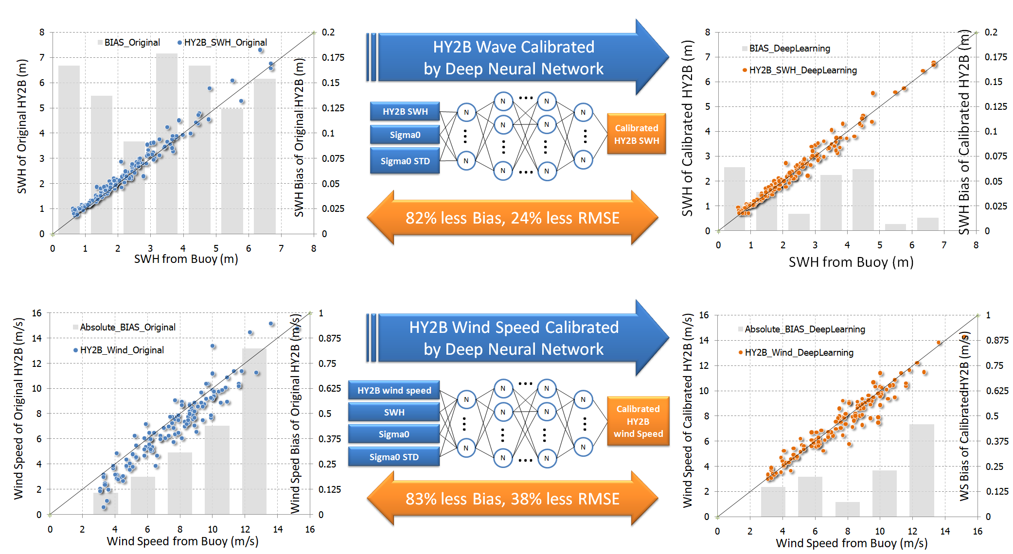
The Geophysical Data Record (GDR) data of HY2B are used in this paper, including 1 Hz along-track observations with SWH, wind speed, and also the sigma0 and sigma0 standard deviation (STD), which is calculated from 20 Hz measurement. The wave and wind observations of the same time period from National Data Buoy Center (NDBC) buoys are used as the truth for the training and validation. As shown in Figure 1, we used a total of 45 buoys data in this paper. To remove the land effect on altimeter signal, only the buoys with distance off shore distance greater than 60 km are considered. These buoys provide hourly SWH and 10 min wind speed observations.

Buoy validation is the first step in verifying the quality of HY2B wind and wave data. The observations from the HY2B and NDBC buoys are mapped according to the following rules: in spatial, we only keep the nearest altimeter footprint from the buoy location and also the distance between the crossovers is considered to be less than 50 km. In the time matching of SWH, the gap between the SWH observation time of the altimeter and the buoys must be less than 1 h (±30 min); while the time resolution of buoys’ wind observation is 10 min. We then reduced the matching time of wind speed from buoys and HY2B to 10 min.

To evaluate the quality of HY2B data, statistical analysis based on the bias, mean absolute error (MAE), normalized root mean square error (NRMSE), root mean square error (RMSE), and scatter index (SI) is implemented. These statistical parameters are defined as follows:

$$bias=\frac{{\displaystyle {\sum }_{i=1}^N(T_i-T_{Ni})}}{N}$$

(4)

$$MAE=\frac{{\displaystyle {\sum }_{i=1}^N|T_i-T_{Ni}|}}{N}$$

(5)

$$NRMSE=100\%\times \frac{\sqrt{{\displaystyle {\sum }_{i=1}^N{(T_i-T_{Ni})}^2}/N}}{\overline{T_{Ni}}}$$

(6)

$$RMSE=\sqrt{\frac{{\displaystyle {\sum }_{i=1}^N{(T_i-T_{Ni})}^2}}{N}}$$

(7)

$$SI=100\%\times \frac{\sqrt{{\displaystyle {\sum }_{i=1}^N[(T_i-\overline{T})-{(T_{Ni}-{\overline{T}}_N)}^2}/N}}{\overline{T_N}}$$

(8)

where the represents the SWH or wind speed from HY2B and is the matched NDBC observation respectively.

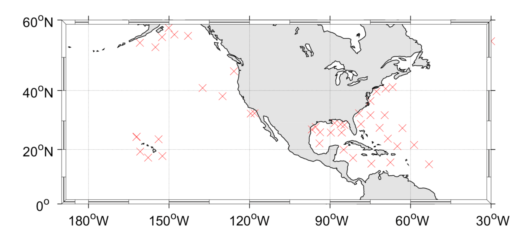
Figure 2 shows the assessment of the HY2B SWH from L2 GDR products. From the scatter diagram in Figure 2a, the HY2B has a good accuracy of SWH with RMSE of roughly 0.23 m and scatter index of 9.4%. However, there is an obvious positive bias of 0.14 m, which induces an NRMSE of 12.1%. We investigated the variation of the bias and SI with the SWH ranges, as illustrated in Figure 2b,c. Six SWH range has been considered. We can clearly see that the positive bias is observed for all SWH ranges. The bias starts from 0.21 for small waves and decreases to 0.12 m for SWH between 5 and 6 m. We also remarked the increase of RMSE from 0.18 m for SWH range of 1 to 2 m to 0.45 m for SWH range greater than 5 m. The SI and NRMSE variation is shown in Figure 2c. We can see that the SI is quite good when SWH is greater than 1 m, with roughly smaller than 9%. On the other hand because of the positive bias, the NRMSE is larger than SI in each SWH ranges.

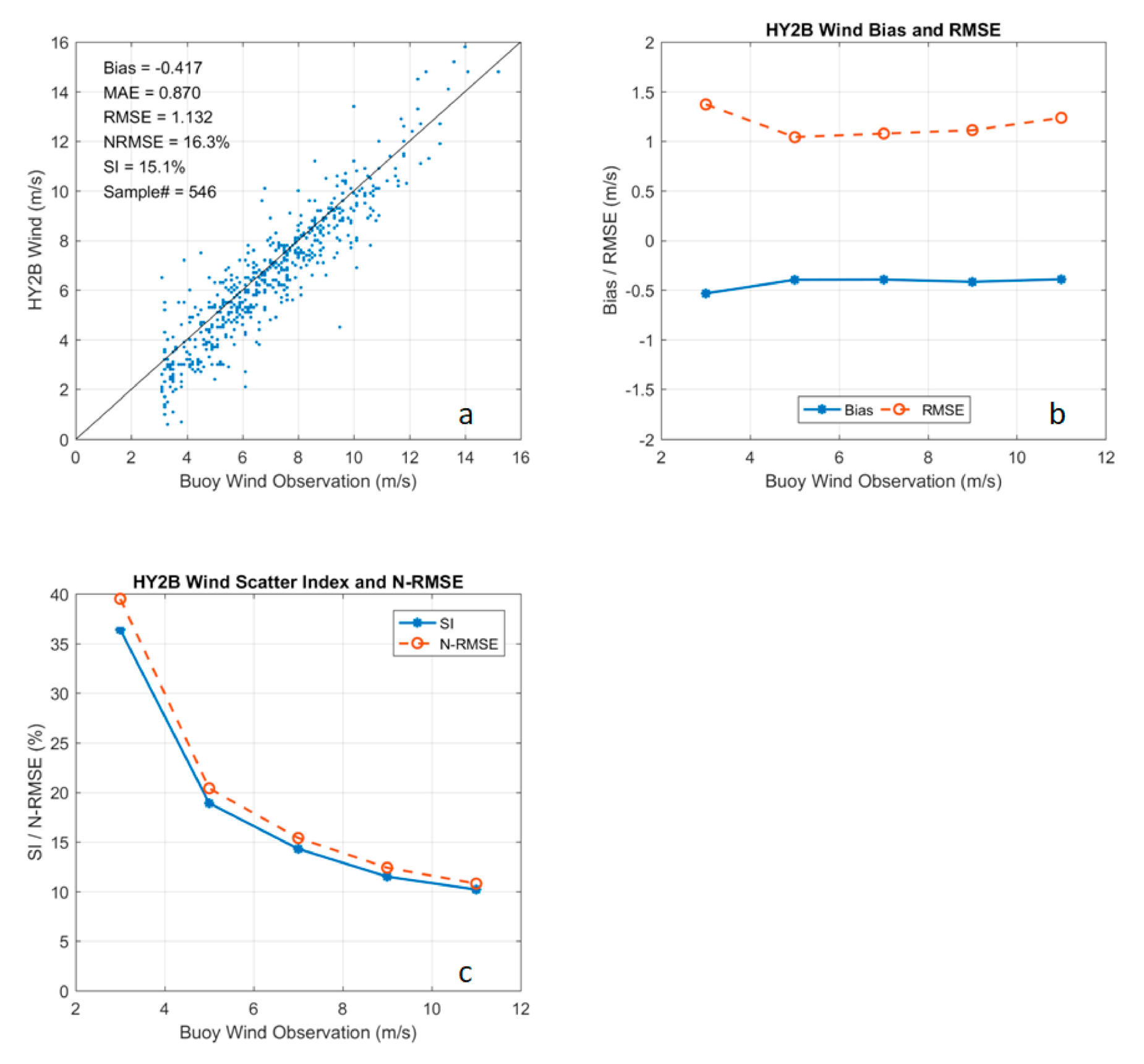
The validation of HY2B wind speed is indicated in Figure 3. The wind speed has a good accuracy compared to NDBC observation, with RMSE of 1.13 m/s. However there is a significant negative bias of −0.42 m/s. The SI and NRMSE are approximately of 15.1% and 16.3%, respectively. The variations of bias and RMSE of HY2B wind speed are shown in Figure 3b. It is can be found that the negative bias is constant for all wind speed ranges, which is easy to recover. The bias is in the range of −0.54 m/s to −0.39 m/s, while the RMSE is roughly of 1 m/s, except that when wind speed is smaller than 4 m/s, where the RMSE increases to 1.37 m/s. Figure 3c shows that the SI and NRMSE decrease with the increase of wind speed. When wind speed larger than 4 m/s, the SI is smaller than 20% and decreases to roughly 10.8% for wind speed larger than 10 m/s. Because of the significant negative bias, the NRMSE is slightly larger than SI.

3. Calibration of HY2B Wave SWH

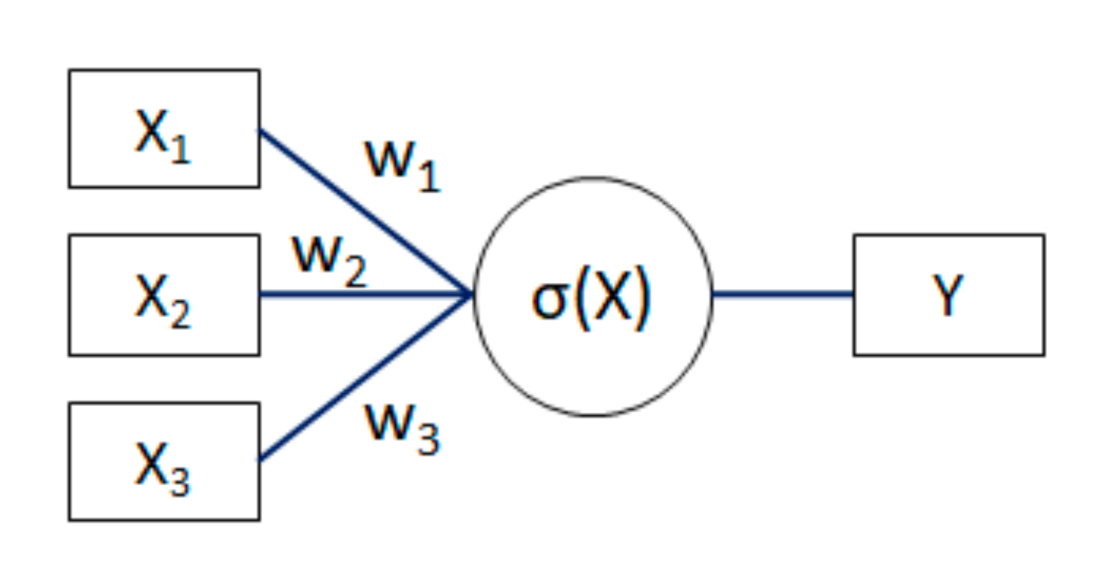
Known from Figure 2, the bias and RMSE change with the SWH. In this section, a deep neural network (DNN) is constructed to calibrate the HY2B original SWH with the SWH and other altimeter parameters as the inputs. The DNN is made up of a certain number of neurons working as follows:

Indicated as Figure 4, the output Y is calculated from:

$$Y=\sigma ({\displaystyle \sum _{i=1}^3{W}_i{X}_i+b)}$$

(9)

where $b$ is the undetermined coefficient. The activation function used in this paper is ReLU (rectified linear unit) [25,26], which is defined as:

$$\sigma (X)=\max (0,X)$$

(10)

The coefficients of weights Wi and b can be determined by so-called supervised training, which is performed following the BP (back propagation) method [27] that is based on the matches of the altimeter parameters and NDBC SWH observations.

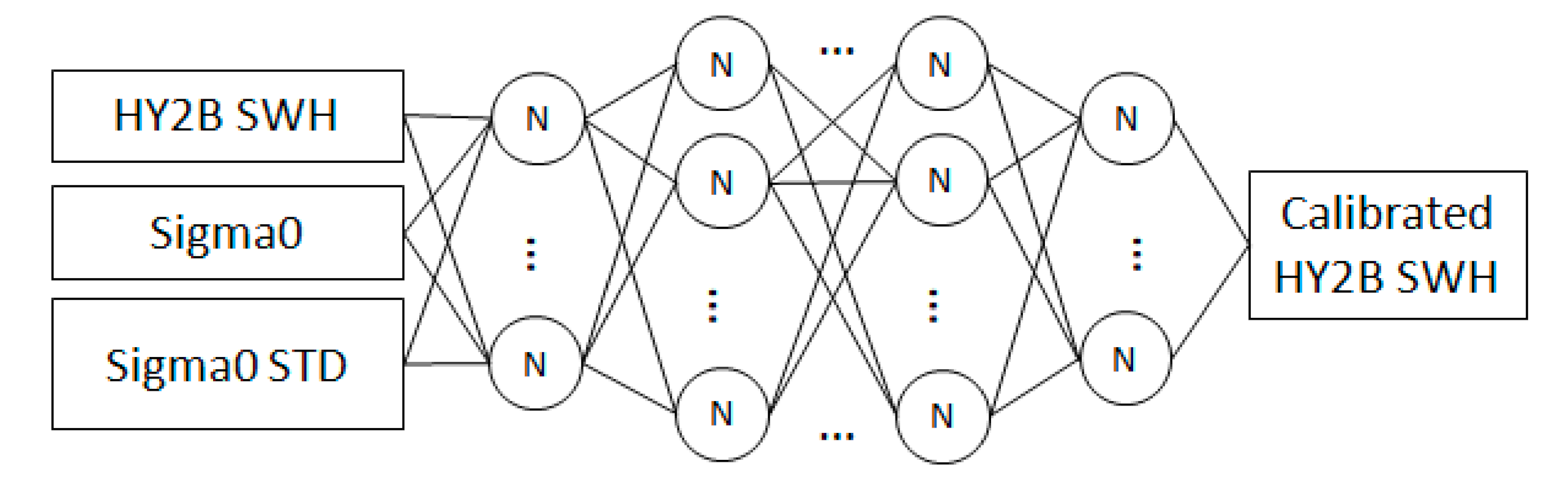
Formed by a set of neurons as in Figure 4, the structure diagram of the SWH calibration DNN is shown in Figure 5. This model is formed by multi-layers (4 layers for SWH calibration) of neurons with the ReLU is used as the activation function in each neuron. Then the input of the DNN model should be determined by selecting the parameters which contain the information of wave height. Beside the SWH, the altimeter also provide other parameters such as sigma0 and simga0 STD. It is known that the sigma0 is highly related to the wind, which is the driving force for the wave; Sigma0 STD is calculated from 20 Hz sigma0, which can be seen as the measurement of sigma0 stability. With these parameters as inputs, DNN will refine the information from these inputs to calibrate the HY2B SWH through its training. Therefore we established three schemes for tests and look for the best combination of inputs, as summarized in

Table 1. Input schemes of deep neural network (DNN) for SWH calibration.

Scheme	Inputs of Deep Neural Network
1	SWH
2	SWH, Sigma0
3	SWH, Sigma0, Sigma0 STD

.

The dataset for the training of DNN contains the SWH, Sigma0, Sigma0 STD from HY2B altimeter and with the matched buoy observed SWH. We can note that the number of matches of high waves is much smaller than that of small waves because of their rare occurrences. For instance, among the HY2B matches there are only 30 matches when SWH exceeds 4 m while there are 159 matches in the SWH range from 2 to 4 m. To ensure a balance of occurrences in the dataset and to avoid any bias in the training of the DNN for SWH calibration, we simply repeat the data matches of rare occurrence several times in order to reach a roughly balanced number. For example, for the SWH beyond 4 m, it would be repeated five times and leads to a balanced number of matches of 150, which is close to 159 matches for “2 to 4 m” section.

The training of DNN is based on the dataset of year 2019 (1st April to 31st December) and we used the data of year 2020 (1st January to 30th April) for independent validation. The training is performed by minimizing the loss between the output of DNN and the matched SWH from buoy. The training is stopped when it reached a required level of loss. The loss function used in training is mean square error (MSE), the optimizer is adam which is an adaptive learning rate optimization algorithm [28]. The training is performed according to three schemes and finally obtains three DNN models for SWH calibration depending on the different inputs. All of the following results are based on the independent validation, using data from the year 2020. Because the validation dataset is a subset of whole HY2B dataset, the statistical results of the original HY2B SWH will be somewhat different from those in Figure 2, but in a limited way.

Table 2. Validation of SWH calibration DNN schemes (Sample# 199).

Scheme	Bias(m)	RMSE(m)	Scatter Index (%)	NRMSE (%)
Original	0.146	0.265	9.8	11.8
1	0.027	0.221	9.7	9.8
2	−0.030	0.214	9.4	9.5
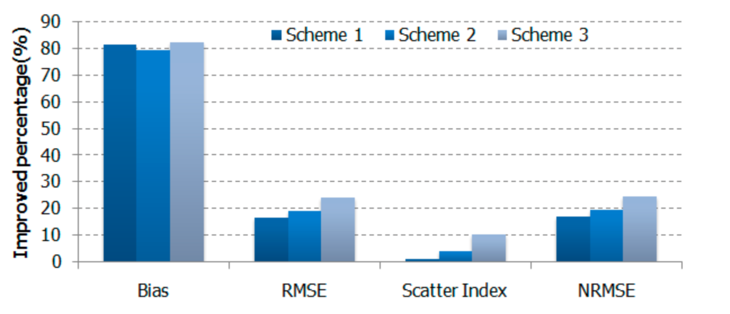
3	0.026	0.201	8.8	8.9

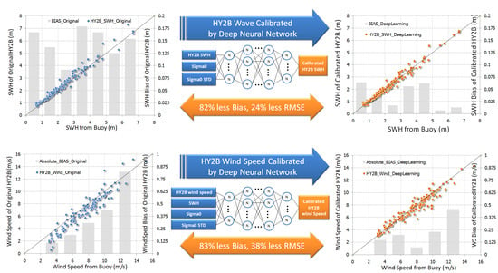
and Figure 6 show the errors reduction results by each DNN calibration schemes. For scheme 1, which uses only the HY2B original SWH as DNN input, the effect is that of linear regression calibration. Scheme 1 can remove 81.5% bias and 16.6% RMSE, but only improve 1% of scatter index. For Scheme 2, when we add sigma0 as input, the correction by DNN is enhanced and improves RMSE and SI by 19.2% and 4%, respectively. For Scheme 3, when we used three inputs by adding sigma0 STD the DNN gives the best calibration. Scheme 3 of DNN has improved RMSE and SI by 24.2% and 10.2%, respectively. This is remarkable because the original SI of HY2B of SWH is already small by roughly 9.8%. It is also noteworthy that all three schemes have succeeded to reduce the bias by approximately 80%.

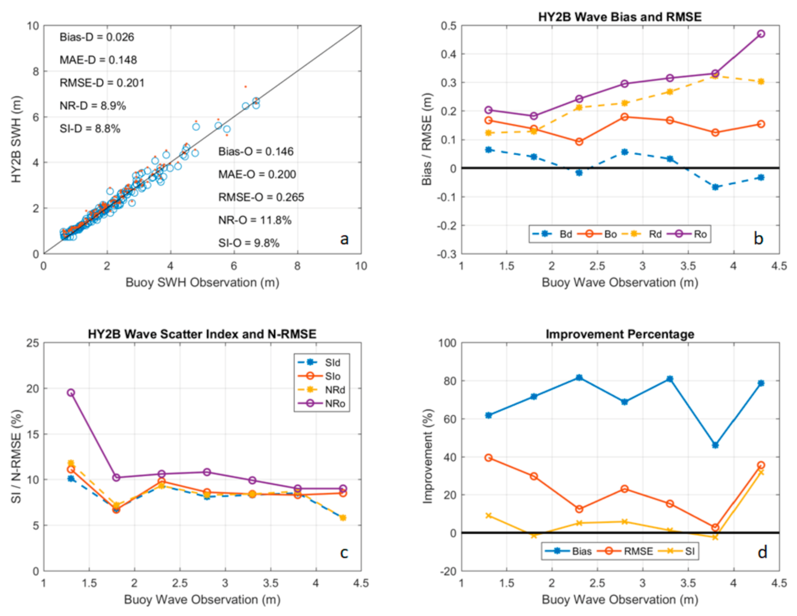
Indicated by Figure 7a, the calibrated SWH by DNN scheme 3 obtains more concentrated distribution scatters than original HY2B SWH, and also eliminates the positive bias. As shown in Figure 7b, the solid lines indicate the HY2B original SWH bias and RMSE distribution while the dotted lines indicate the calibrated SWH bias and RMSE distribution. As analyzed in Figure 2, the original HY2B SWH has an obvious positive bias (solid orange line) in all SWH range, the DNN can effectively remove most of its bias, make the calibrated bias distributed around 0 m (blue dotted line); the DNN also significantly reduced the RMSE of original HY2B SWH (solid purple line) in all SWH range. In Figure 7c, we can also find that the DNN make the distribution of SI and NRMSE from calibrated SWH (blue and yellow dotted lines, respectively) lower than that from original HY2B SWH (red and purple solid lines, respectively). It is should be noted that, because the DNN removes most of the bias, the SI and NRMSE of calibrated SWH nearly coincide to each other. Figure 7d shows the percentage of improvement by the calibration DNN. We can find that the DNN has removed 60% to 80% bias in all SWH range. The improvement in NRMSE and SI is not stable, more improvements are found when SWH is less than 1.5 m and larger than 4 m, in the section of 1.5 to 2 m and 3.5 to 4 m the DNN degrade the SI insignificantly but still improved in NRMSE. Overall, we can infer that the sigma0 STD should be considered into the calibration of SWH, it helps the calibration DNN to effectively reduce the errors of the original HY2B SWH, including most of the bias, 24% of the RMSE and NRMSE, and 10% of the SI.

4. Calibration of HY2B Wind Speed

Having obtained the promising calibration result by using DNN in SWH, we performed another experiment of wind speed calibration based on DNN. The parameters of altimeter besides the HY2B original wind speed are used as the input of the DNN for calibration. It is pointed out that the wave SWH should also be included in the calculation of wind speed beside the sigma0 [29]. Therefore we include the HY2B wind speed, sigma0, SWH, and sigma0 STD into the DNN, which enables a good calibration by refining the information from these inputs. The structure diagram of the SWH calibration DNN is shown as Figure 8. The basic structure of wind DNN model is similar as SWH DNN, which is formed by five layers of neurons. The activation function is also the ReLU. The loss function used in training is MSE, the optimizer is adam.

Table 3. Input schemes of DNN for wind calibration (Sample# 127).

Scheme	Inputs of Deep Neural Network	Input Para. Number
1	wind speed	1
2	wind speed, Sigma0	2
3	wind speed, SWH	2
4	wind speed, Sigma0 STD	2
5	wind speed, sigma0, sigma0 STD	3
6	wind speed, SWH, sigma0, sigma0 STD	4

shows the setup of the schemes for HY2B wind speed calibration DNN. Because there are three other parameters (beside the original wind speed of HY2B) that may contain helpful information to reduce the error of wind speed, there are a total of six schemes with different combination of inputs that are tested to obtain the best DNN scheme. The dataset for the training of calibration DNN is also formed based on the matches between HY2B and NDBC buoy wind speed observation, i.e., using the data of year 2019 as the training dataset while using the data of year 2020 as independent validation dataset. The dataset for the training of DNN contains the original wind speed, SWH, Sigma0, Sigma0 STD from HY2B altimeter and with the matched buoy wind speed. Like the balance process used in SWH dataset in Section 3, the wind speed dataset should be also balanced in the data number of each section of wind speed because of the difference in the occurrences of different wind speed.

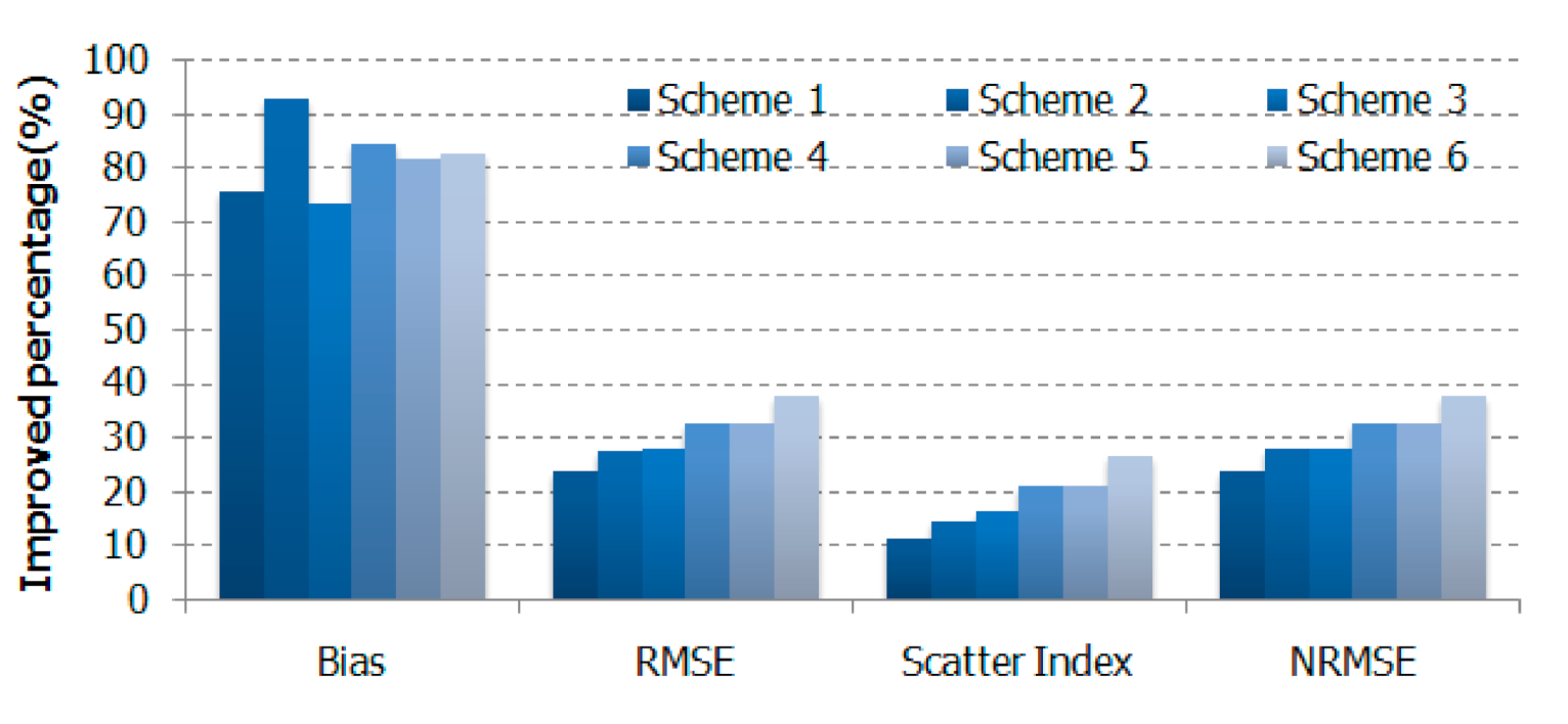
The training of DNN is performed according to these six schemes and allows to finally obtain their wind speed calibration results. The statistical results are show in

Table 4. Validation of wind speed calibration DNN schemes.

Scheme	Bias (m/s)	RMSE (m/s)	Scatter Index (%)	NRMSE (%)
Original	−0.584	1.099	12.4	14.7
1	−0.141	0.839	11.0	11.2
2	−0.042	0.796	10.6	10.6
3	−0.155	0.792	10.4	10.6
4	−0.090	0.741	9.8	9.9
5	−0.106	0.742	9.8	9.9
6	−0.100	0.686	9.1	9.2

and the improvement percentage of each scheme is shown in Figure 9. Overall, the scheme with more input gets better calibration accuracy. Scheme 1 only has original wind speed as the input, and is more focused on bias reduction, meanwhile show a least decrease in the SI or NRMSE; when comparing the scheme 2, 3, 4, they all use two inputs that with sigma0, SWH and sigma0 STD, respectively. It can be seen that although adding another parameter can help to have better calibration, the addition of sigma0 STD gets the best improvement than SWH and sigma0 itself. When we add the sigma0 STD into DNN, the calibration can decrease 32.6% of RMSE and improve SI by 21%! It is reasonable because the wind speed of original HY2B altimeter is calculated by using the algorithm with sigma0 and SWH as the input, so the amount of new information provided by SWH and sigma0 is limited. Meanwhile, it should be noted that the parameter sigma0 STD should be considered as a key factor in wind speed calibration. Therefore it is not surprising to obtain the best calibration results for wind when using all four parameters as the input of DNN, as Scheme 6.

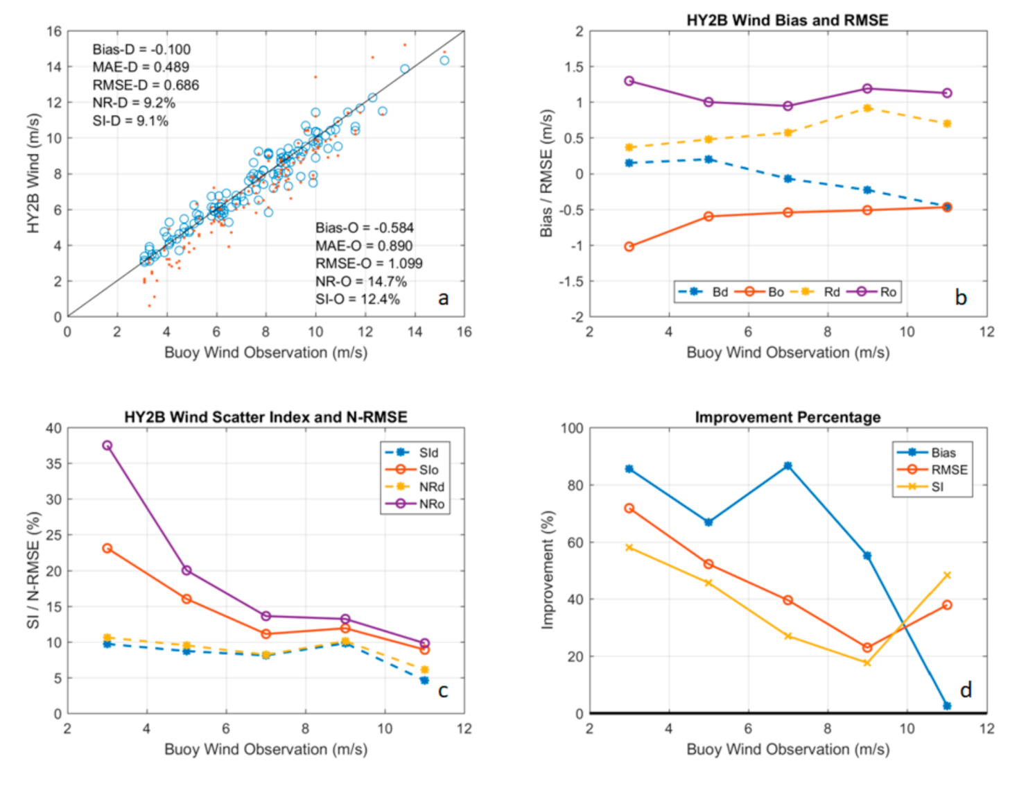
Indicated by Figure 10a, the DNN using scheme 6 significantly improved the scatter distribution and mostly removed the bias. As shown in Figure 10b, the DNN calibrated wind speed obtained less bias (blue dotted line) than original data (red solid line) when wind speed was under 8 m/s, although there is negative bias in calibrated when wind speed is beyond 8 m/s, the absolute vale of bias is still smaller than the original HY2B wind speed; in all wind speed range, the RMSE of calibrated wind speed (yellow dotted line) is less than that of original wind speed (purple solid line). As shown in Figure 10c, the SI and NRMSE are significantly reduced after the calibration by DNN. The SI and RMSE distribution line through calibration (blue and yellow dotted line) matched well because limited bias exists. Figure 10d gives the improvement percentage distribution of bias, RMSE, and SI. It can be seen that the DNN effectively reduced the RMSE and SI in low wind that is under 6 m/s, which gives relative obvious error. One should note that even in the range 8 to 10 m/s, DNN still decreases around 20% of RMSE and SI, which is remarkable. Therefore the DNN is able to give nice calibration of wind speed with refining the information from SWH, sigma0, and especially sigma0 STD.

5. Discussion and Conclusions

HY2B altimeter is now the latest mission of altimetry. The validation of HY2B wind speed and SWH is carried out against the observations of NDBC buoy. From the assessment based on 1-year time-space matched data, HY2B SWH gives a good accuracy with positive bias of 0.143 m and 9.4% SI. The bias of HY2B maintains positive around 0.15 m, while the SI keeps under 10% when SWH is greater than 1 m. For HY2B altimeter wind speed the statistical analysis shows a negative bias of −0.417 m/s, and SI of 15.1%. The wind speed bias is constant for all wind speed ranges, while the SI is increased when wind speed is smaller than 6 m/s. However for wind speed that is above 6 m/s, the SI is less than 15%. To improve the accuracy of HY2B data, a deep learning technique has been implemented. Several schemes of DNN have been built. The DNN calibration shows a significant improvement of statistical parameters (bias, RMSE, and SI) of SWH and wind speed. Regarding to SWH calibration, the use of three inputs, SWH, sigma0, and sigam0 STD, in the DNN reduced significantly the bias by 80%, RMSE by 24%, and SI by 10% of SI. For wind speed calibration the same DNN is also applied with additional learning information from HY2B wind speed. The wind speed has been significantly improved by 82% for the bias, 38% for RMSE, and 27% for SI.

The deep learning technique has proved the good ability and robustness for the calibration of HY2B. The DNN model has indicated the skillfulness of the sigma0 STD to correct both SWH and wind speed from altimeters. This opens a good perspective to extend the DNN model to other altimeters missions. The correction of HY2B SWH and wind speed will be very useful for the development in future global and regional wave reanalysis in terms of validation and assimilation in models.

An important revelation from above is that many parameters of the altimeter observation (sigma0 STD, etc.,) contain the positive information that could be well refined by the approach of deep learning, hence they will be helpful in improving the accuracy of the altimeter retrieval and should be considered in the calibration phase of altimeters or other remote sensing missions.

Finally, we want to emphasize that the implementation of calibration based on deep learning requires special attention. This concerns the over fitting that can be caused by DNN. Because the validation and calibration processes are more likely performed on the matches between altimeter and buoy, the number of observation is always quite limited, so the DNN should be carefully designed, such as the number of layers and neurons, and then fully tested on an independent dataset to obtain the best calibration.

References

- Fedor, L.S.; Godbey, T.W.; Gower, J.F.R.; Guptill, R.; Hayne, G.S.; Rufenach, C.L.; Walsh, E.J. Satellite altimeter measurements of sea state—An algorithm comparison. J. Geophys. Res. Solid Eart 1979, 84, 3991–4001. [Google Scholar] [CrossRef]
- Brown, G. The average impulse response of a rough surface and its applications. IEEE Trans. Antennas Propag. 1977, 25, 67–74. [Google Scholar] [CrossRef]
- Hayne, G. Radar altimeter mean return waveforms from near-normal-incidence ocean surface scattering. IEEE Trans. Antennas Propag. 1980, 28, 687–692. [Google Scholar] [CrossRef] [Green Version]
- Dobson, E.; Monaldo, F.; Goldhirsh, J.; Wilkerson, J. Validation of Geosat altimeter-derived wind speeds and significant wave heights using buoy data. J. Geophys. Res. Ocean. 1987, 92, 10719–10731. [Google Scholar] [CrossRef]
- Rodríguez, E.; Chapman, B. Extracting ocean surface information from altimeter returns: The deconvolution method. J. Geophys. Res. Ocean. 1989, 94, 9761–9778. [Google Scholar] [CrossRef]
- Nerem, R.S.; Chambers, D.P.; Choe, C.; Mitchum, G.T. Estimating mean sea level change from the TOPEX and Jason altimeter missions. Mar. Geod. 2010, 33, 435–446. [Google Scholar] [CrossRef]
- Lee, H.; Shum, C.K.; Emery, W.; Calmant, S.; Deng, X.; Kuo, C.-Y.; Roesler, C.; Yi, Y. Validation of Jason-2 altimeter data by waveform retracking over California coastal ocean. Mar. Geod. 2010, 33, 304–316. [Google Scholar] [CrossRef]
- Yang, J.; Zhang, J.; Jia, Y.; Fan, C.; Cui, W. Validation of Sentinel-3A/3B and Jason-3 Altimeter Wind Speeds and Significant Wave Heights Using Buoy and ASCAT Data. Remote Sens. 2020, 12, 2079. [Google Scholar] [CrossRef]
- Liu, Q.; Babanin, A.V.; Guan, C.; Zieger, S.; Sun, J.; Jia, Y. Calibration and validation of HY-2 altimeter wave height. J. Atmos. Ocean. Technol. 2016, 33, 919–936. [Google Scholar] [CrossRef] [Green Version]
- Jiang, M.; Xu, K.; Liu, Y. Global statistical assessment and cross-calibration with Jason-2 for reprocessed HY-2 A altimeter data. Mar. Geod. 2018, 41, 289–312. [Google Scholar] [CrossRef]
- Cotton, P.D.; Carter, D.J.T. Cross calibration of TOPEX, ERS-I, and Geosat wave heights. J. Geophys. Res. Ocean. 1994, 99, 25025–25033. [Google Scholar] [CrossRef]
- Torres, R.; Snoeij, P.; Geudtner, D.; Bibby, D.; Davidson, M.; Attema, E.; Potin, P.; Rommen, B.; Floury, N.; Brown, M. GMES Sentinel-1 mission. Remote Sens. Environ. 2012, 120, 9–24. [Google Scholar] [CrossRef]
- Hauser, D.; Xiaolong, D.; Aouf, L.; Tison, C.; Castillan, P. Overview of the CFOSAT mission. In Proceedings of the 2016 IEEE International Geoscience and Remote Sensing Symposium (IGARSS), Beijing, China, 10–15 July 2016; pp. 5789–5792. [Google Scholar]
- Abdalla, S.; Janssen, P.A.E.M.; Bidlot, J.-R. Jason-2 OGDR wind and wave products: Monitoring, validation and assimilation. Mar. Geod. 2010, 33, 239–255. [Google Scholar] [CrossRef]
- Lionello, P.; Günther, H.; Janssen, P.A.E.M. Assimilation of altimeter data in a global third-generation wave model. J. Geophys. Res. Ocean. 1992, 97, 14453–14474. [Google Scholar] [CrossRef]
- Breivik, L.-A.; Reistad, M. Assimilation of ERS-1 altimeter wave heights in an operational numerical wave model. Weather Forecast. 1994, 9, 440–451. [Google Scholar] [CrossRef] [Green Version]
- Jiang, H.; Stopa, J.E.; Wang, H.; Husson, R.; Mouche, A.; Chapron, B.; Chen, G. Tracking the attenuation and nonbreaking dissipation of swells using altimeters. J. Geophys. Res. Ocean. 2016, 121, 1446–1458. [Google Scholar] [CrossRef] [Green Version]
- Young, I.R.; Babanin, A.V.; Zieger, S. The decay rate of ocean swell observed by altimeter. J. Phys. Oceanogr. 2013, 43, 2322–2333. [Google Scholar] [CrossRef]
- Jiang, H.; Chen, G. A global view on the swell and wind sea climate by the Jason-1 mission: A revisit. J. Atmos. Ocean. Technol. 2013, 30, 1833–1841. [Google Scholar] [CrossRef]
- Barth, A.; Alvera-Azcarate, A.; Licer, M.; Beckers, J.-M. DINCAE 1.0: A convolutional neural network with error estimates to reconstruct sea surface temperature satellite observations. Geosci. Model Dev. 2020, 13, 1609–1622. [Google Scholar] [CrossRef] [Green Version]
- Song, T.; Jiang, J.; Li, W.; Xu, D. A deep learning method with merged LSTM Neural Networks for SSHA Prediction. IEEE J. Sel. Top. Appl. Earth Obs. Remote Sens. 2020, 13, 2853–2860. [Google Scholar] [CrossRef]
- Rasp, S.; Dueben, P.D.; Scher, S.; Weyn, J.A.; Mouatadid, S.; Thuerey, N. WeatherBench: A benchmark dataset for data-driven weather forecasting. arXiv 2020, arXiv:2002.00469. [Google Scholar]
- Jia, Y.; Lin, M.; Zhang, Y. Evaluations of the Significant Wave Height Products of HY-2B Satellite Radar Altimeters. Mar. Geod. 2020, 1–18. [Google Scholar] [CrossRef]
- Gourrion, J.; Vandemark, D.; Bailey, S.; Chapron, B.; Gommenginger, G.P.; Challenor, P.G.; Srokosz, M.A. A two-parameter wind speed algorithm for Ku-band altimeters. J. Atmos. Ocean. Technol. 2002, 19, 2030–2048. [Google Scholar] [CrossRef]
- Xu, B.; Wang, N.; Chen, T.; Li, M. Empirical evaluation of rectified activations in convolutional network. arXiv 2015, arXiv:1505.00853. [Google Scholar]
- Nair, V.; Hinton, G.E. Rectified linear units improve restricted boltzmann machines. In Proceedings of the ICML, Haifa, Isreal, 21–24 June 2010. [Google Scholar]
- Witten, I.H.; Frank, E. Data mining: Practical machine learning tools and techniques with Java implementations. AcmSigmod Rec. 2002, 31, 76–77. [Google Scholar] [CrossRef]
- Kingma, D.P.; Ba, J. Adam: A method for stochastic optimization. arXiv 2014, arXiv:1412.6980. [Google Scholar]
- Lefevre, J.M.; Barckicke, J.; Menard, Y. A significant wave height dependent function for TOPEX/POSEIDON wind speed retrieval. J. Geophys. Res. Ocean. 1994, 99, 25035–25049. [Google Scholar] [CrossRef]
Figure 1.
The locations of National Data Buoy Center (NDBC) buoys used in the paper.
Figure 2.
The validation of HY2B significant wave height (SWH) against NDBC buoys. (a) Indicates the scatters and the statistical parameters; (b) indicates the bias and RMSE distribution with the SWH value; (c) indicates the scatter index (SI) and normalized root mean square error (NRMSE) distribution with the SWH value.
Figure 3.
The validation of HY2B wind speed against NDBC buoys. (a) Indicates the scatters and the statistical parameters; (b) indicates the bias and RMSE distribution with the wind speed;(c) indicates the SI and NRMSE distribution with the wind speed.
Figure 4.
The basic calculation principle of one neuron. X1, X2, and X3 are the input of the neuron; W1, W2, and W3 are the weight of each input X; the activation function of the neuron is σ(X); Y is the output of the neuron.
Figure 5.
The structure of deep neural network for SWH calibration scheme 3.
Figure 6.
The percentage of the reduction of error by each SWH calibration DNN scheme.
Figure 7.
Detailed comparison between the DNN scheme 3 and original HY2B SWH. (a) Shows scatter plots of SWH from buoys and HY2B. Red dots and blue circles stand for original HY2B and DNN calibration, respectively; (b) shows the bias and RMSE variation with SWH, Bd, and Bo indicate the bias of DNN calibration and original HY2B, respectively, Rd and Ro represent the RMSE of DNN and original. While (c) shows the SI and NRMSE variation with SWH, SId and SIo stand for SI of DNN and original; NRd and NRo stand for NRMSE of DNN and original; (d) shows the percentage of improvement by the DNN calibration for bias, RMSE, and SI.
Figure 8.
The structure of deep neural network for wind speed calibration scheme 6.
Figure 9.
The percentage of the reduction of error by each wind speed calibration DNN scheme.
Figure 10.
Detailed comparison between the DNN scheme 6 and original HY2B wind speed. (a) Shows the scatter plots of original HY2B wind speed (red dots) and DNN-calibrated wind speed (blue cycles); (b) shows the bias and RMSE distribution with the wind speed. Bd and Bo represent the bias of DNN calibration and original HY2B, respectively. Rd and Ro stand forRMSE of DNN and original; (c) shows the SI and NRMSE variation with wind speed, SId and SIo represent the SI of DNN and original while NRd and NRo represent the NRMSE of DNN and original. (d) shows the percentage of improvement by the DNN calibration for bias, RMSE and SI.